เริ่มต้นอย่างรวดเร็ว

---

title: Quickstart description: คู่มือเริ่มต้นอย่างรวดเร็วสำหรับแพ็กเกจ pauli-prop ของ Qiskit addons

ในคู่มือนี้ เราใช้แพ็กเกจ pauli-prop เพื่อจำลองพลวัตเชิงเวลาของโมเดล kicked Ising 10 ควอนตัมบิตบนสายสปิน 1 มิติด้วยคอมพิวเตอร์แบบคลาสสิก

เตรียมอินพุตสำหรับ Pauli propagation

แฮมิลโทเนียนที่พิจารณาคือ:

$H = -J\sum\limits_{\langle i,j \rangle} Z_iZ_j + h\sum\limits_iX_i$

โดยที่ $J>0$ อธิบายการคับปลิงของสปินที่อยู่ใกล้กันที่สุด, $i<j$ และ $h$ คือสนามตามขวางส่วนกลาง การแยกส่วนแบบ Trotter อันดับหนึ่งของตัวดำเนินการที่วิวัฒน์ตามเวลาจะถูกสร้างเป็นควอนตัมเซอร์กิต $U$ ตลอด $20$ ขั้นของ Trotter ค่าคงที่การคับปลิง $J$ จะถูกกำหนดเป็น $J=-\frac{\pi}{2}$ และ $h$ จะถูกกำหนดเป็น $\frac{\pi}{6}$ ปฏิสัมพันธ์ $ZZ$ จะถูกสร้างโดยใช้เกต Clifford ($CX$, $Sdg$, $\sqrt{Y}$)

เราสร้างวิวัฒนาการเชิงเวลาแบบ Trotter เป็นควอนตัมเซอร์กิต และใช้ $\frac{\pi}{6}$ สำหรับการหมุนที่ไม่ใช่ Clifford รอบแกน x ยิ่งมุมเหล่านี้อยู่ห่างจากมุม Clifford (เช่น $\theta=n\frac{\pi}{2}, n \in \mathbb{Z}$) มากเท่าไร ระบบก็จะยิ่งจำลองยากขึ้นสำหรับวิธี Pauli propagation

สำหรับการเลือกออบเซอร์เวเบิล เราพิจารณาแมกนีไทเซชันเฉลี่ยต่อไซต์เดี่ยว $\frac{1}{N} \sum_{i=1}^{N} \langle z_i \rangle$ โดยที่ $N$ คือจำนวนสปิน

# Added by doQumentation — installs the packages this notebook needs if they are missing
import importlib.util

_needed = {"matplotlib": "matplotlib", "numpy": "numpy", "pauli_prop": "pauli-prop", "qiskit": "qiskit", "qiskit_aer": "qiskit-aer"}
_missing = [pip for module, pip in _needed.items()
            if importlib.util.find_spec(module) is None]
# One at a time, so a package that fails to install does not block the others
for _pip in _missing:
    %pip install -q {_pip}
if not _missing:
    print("\u2713 All required packages are installed")

import numpy as np
from qiskit import QuantumCircuit
from qiskit.quantum_info import SparsePauliOp
from qiskit.transpiler import CouplingMap

num_qubits = 10
coupling_map = CouplingMap.from_line(num_qubits, bidirectional=False)

# Num Trotter steps
num_steps = 20
theta_rx = np.pi / 6

# Average single-site magnetization
observable = (
    SparsePauliOp(
        [
            "I" * iq + "Z" + "I" * (num_qubits - iq - 1)
            for iq in range(num_qubits)
        ]
    )
    / num_qubits
)

# Create the Trotter circuit
num_qubits = 10
num_steps = 20
theta_rx = np.pi / 6
circuit = QuantumCircuit(num_qubits)
edges = CouplingMap.from_line(num_qubits, bidirectional=False).get_edges()
for _ in range(num_steps):
    circuit.rx(theta_rx, [i for i in range(num_qubits)])
    for edge in edges:
        circuit.sdg(edge)
        circuit.ry(np.pi / 2, edge[1])
        circuit.cx(edge[0], edge[1])
        circuit.ry(-np.pi / 2, edge[1])
circuit.draw("mpl", fold=-1)

จำลองวิวัฒนาการเชิงเวลาของระบบด้วย Pauli propagation

เมื่อเรามีเซอร์กิต $U$ และออบเซอร์เวเบิล $O$ แล้ว เราก็สามารถจำลองระบบได้อย่างง่ายดายในไม่กี่ขั้นตอน:

• แยก $U$ ออกเป็นส่วน Clifford $C$ และส่วนที่ไม่ใช่ Clifford $P$ โดยที่ $U=PC$ ด้วย evolve_through_cliffords

• แพร็อพาเกต $O$ ผ่าน $P$ ได้ตัวดำเนินการใหม่ $O^\prime$ โดยใช้ pauli_prop.propagate_through_circuit

• วิวัฒน์ $O^\prime$ ผ่านส่วน Clifford ของเซอร์กิตโดยใช้การรองรับวิวัฒนาการแบบ Clifford ที่มีอยู่ใน Qiskit

• ประมาณค่าคาดหมายเป็น $\langle0|O^\prime|0\rangle \approx \langle0|U^\dagger OU|0\rangle$ โดยรวมสัมประสิทธิ์ใน $O^\prime$ ที่เกี่ยวข้องกับพจน์ Pauli แบบทแยงมุมเต็มรูป (พจน์ Pauli ที่มีเพียง I หรือ Z บนทุกควอนตัมบิต) โปรดจำไว้ว่านี่เป็นเพียงค่าประมาณ เพราะเราตัดพจน์บางส่วนออกจาก $O^\prime$ ขณะแพร็อพาเกตผ่านส่วนที่ไม่ใช่ Clifford ของเซอร์กิต

import time

from pauli_prop import evolve_through_cliffords, propagate_through_circuit

cliff, non_cliff = evolve_through_cliffords(circuit)

max_terms_list = [10**i for i in range(8)]
approx_evs = []
durations = []
for max_terms in max_terms_list:
    st = time.perf_counter()
    evolved_obs = propagate_through_circuit(
        observable, non_cliff, max_terms=max_terms, atol=1e-12, frame="h"
    )[0]
    evolved_obs.paulis = evolved_obs.paulis.evolve(cliff, frame="h")
    durations.append(time.perf_counter() - st)
    approx_evs.append(
        float(evolved_obs.coeffs[~evolved_obs.paulis.x.any(axis=1)].sum())
    )

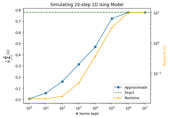
เมื่อเรารันการคำนวณที่ใหญ่ขึ้น ค่าประมาณของค่าคาดหมายก็จะแม่นยำขึ้น ในตัวอย่างนี้ เราอิ่มตัวเต็มปริภูมิ Pauli ที่ประมาณ $4^{10}\approx10^6$ ซึ่งสะท้อนให้เห็นจากเส้นโค้งที่แบนราบลงระหว่างสองจุดสุดท้าย

แม้กราฟด้านล่างจะแสดงการลู่เข้าแบบเอกภาพ แต่การจำลอง Pauli propagation โดยทั่วไปไม่ได้ลู่เข้าแบบเอกภาพเสมอไป การเห็นพฤติกรรมแบบ "ขรุขระ" ในกราฟประเภทนี้ไม่ใช่เรื่องผิดปกติ

import matplotlib.pyplot as plt
from qiskit_aer import AerSimulator

sim_circ = circuit.copy()
sim_circ.save_statevector()
backend = AerSimulator(method="statevector")
psi = backend.run(sim_circ).result().data()["statevector"]
exact_ev = psi.expectation_value(observable)

ax1 = plt.gca()
ax1.plot(max_terms_list, approx_evs, marker="o", label="Approximate")
ax1.axhline(exact_ev, linestyle="--", color="green", label="Exact")
ax1.set_xscale("log")
ax1.set_xlabel("# terms kept")
ax1.set_ylabel(r"$\frac{1}{N} \sum_{i=1}^{N} \langle z_i \rangle$")

ax2 = ax1.twinx()
ax2.plot(
    max_terms_list, durations, marker=".", label="Runtime", color="orange"
)
ax2.set_ylabel("Runtime (s)", color="orange")
ax2.set_yscale("log")

handles1, labels1 = ax1.get_legend_handles_labels()
handles2, labels2 = ax2.get_legend_handles_labels()
ax1.legend(handles1 + handles2, labels1 + labels2, loc="lower right")

plt.title(f"Simulating {num_steps}-step 1D Ising Model")

Text(0.5, 1.0, 'Simulating 20-step 1D Ising Model')