การระงับและปรับแต่งข้อผิดพลาด

การระงับข้อผิดพลาด (error suppression) สามารถหมายถึงเทคนิคใด ๆ ที่คาดการณ์ล่วงหน้าและพยายามหลีกเลี่ยงสัญญาณรบกวนและข้อผิดพลาดบางประเภท วิธีที่ง่ายที่สุดในการอธิบายเรื่องนี้คือผ่านตัวอย่างที่เป็นรูปธรรม แต่โปรดจำไว้ว่าวิธีการเหล่านี้ไม่ได้จำกัดอยู่แค่ตัวอย่างที่แสดงในที่นี้เท่านั้น และมีการสำรวจวิธีการใหม่ ๆ อย่างต่อเนื่อง บางครั้งการระงับข้อผิดพลาดเป็นไปไม่ได้ แต่สามารถส่งผลต่อวิธีที่ข้อผิดพลาดสะสมได้ หากเราสามารถทำให้ข้อผิดพลาดสะสมช้าลงได้ เราอาจอธิบายว่านี่คือการระงับข้อผิดพลาดโดยรวม แต่จริง ๆ แล้วควรมองว่าเป็นการปรับแต่งสัญญาณรบกวน (noise tailoring) มากกว่า ในบทเรียนนี้เราจะครอบคลุมตัวอย่างมาตรฐานของการระงับข้อผิดพลาด (dynamical decoupling) และการปรับแต่ง/กำหนดรูปสัญญาณรบกวน (Pauli twirling)

วิดีโอประกอบบทเรียนนี้จะเผยแพร่ในอีกไม่กี่วันข้างหน้า และจะถูกฝังไว้ที่นี่

Dynamical decoupling

เริ่มต้นด้วยสถานะที่ง่ายมากบน qubit เดี่ยว และแนะนำโมเดลสัญญาณรบกวนอย่างง่าย สิ่งนี้ยังไม่เพียงพอที่จะอธิบาย dynamical decoupling ได้อย่างสมบูรณ์ แต่ก็ให้ตัวอย่างที่ชัดเจนแก่เรา สมมติว่าเรามี qubit ที่ถูกเตรียมในสถานะ superposition โดยใช้ Hadamard gate:

$$|\psi\rangle = H|0\rangle = \frac{1}{\sqrt{2}}\left( |0\rangle +|1\rangle \right).$$

สถานะนี้ถูกแสดงเป็นภาพบน Bloch sphere ดังที่แสดงด้านล่างทางซ้าย ในกรณีที่สมบูรณ์แบบโดยไม่มีสัญญาณรบกวนเลย qubit นี้จะคงอยู่ในสถานะนี้จนกว่าจะมีการดำเนินการครั้งถัดไป อย่างไรก็ตาม เรารู้จากบทเรียนก่อนหน้านี้ว่านี่ไม่ใช่สิ่งที่เราสังเกตเห็น สัญญาณรบกวนทำให้ข้อมูลควอนตัมเสื่อมสภาพ

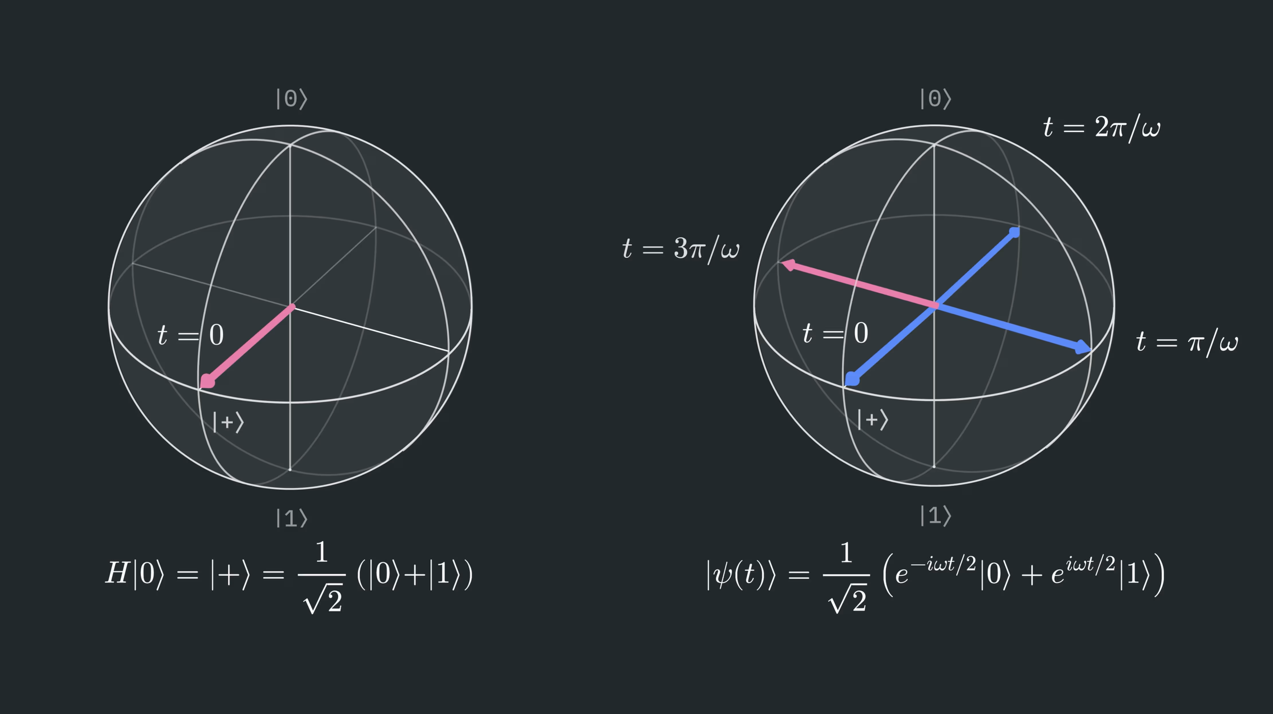
สัญญาณรบกวนหรือการเชื่อมโยงกับสภาพแวดล้อมสามารถทำให้เฟสสัมพัทธ์ระหว่างสถานะฐานเปลี่ยนแปลงได้ นั่นคือ ความน่าจะเป็นของ $|0\rangle$ และ $|1\rangle$ ไม่เปลี่ยนแปลง เนื่องจากค่าสัมบูรณ์ของสัมประสิทธิ์ของสถานะเหล่านั้นไม่เปลี่ยนแปลง แต่เฟสของแอมพลิจูดเปลี่ยนแปลง ทำให้ส่วนจริงและส่วนจินตภาพเปลี่ยนแปลงไป เพื่อให้การอภิปรายนี้เป็นรูปธรรมมากขึ้น ลองพิจารณาปฏิสัมพันธ์ประเภทหนึ่งที่สามารถทำให้เกิดสิ่งนี้ได้ นั่นคือการเชื่อมโยงกับสนามแม่เหล็กที่มีทิศทางในแนวแกน Z: $\vec{B} = (0,0,B_0)$.

ลองพิจารณาว่าเกิดอะไรขึ้นกับสถานะ $|+\rangle$ เมื่อเวลาผ่านไป:

$$|\psi(t)\rangle = e^{-iHt/\hbar}|\psi(0)\rangle \rightarrow e^{-iZ\omega_B t/2}|\psi(0)\rangle$$

ในที่นี้เราใช้ข้อเท็จจริงที่ว่าสนามแม่เหล็กในแนวแกน Z ทำให้เกิดการส่ายรอบแกน Z ด้วยความถี่ $\omega_B$ ซึ่งขึ้นอยู่กับโมเมนต์แม่เหล็กที่มีผลและความแรงของสนามแม่เหล็ก รายละเอียดนั้นมีความสำคัญน้อยกว่าข้อเท็จจริงที่ว่าปฏิสัมพันธ์นี้ทำให้เกิดวิวัฒนาการรอบแกน Z ซึ่งส่งผลให้เกิดการสะสมเฟสในทิศทางตรงข้ามกันสำหรับสถานะฐานเชิงคำนวณทั้งสอง เมื่อนำตัวดำเนินการนี้ไปใช้กับแต่ละเทอมใน $|\psi\rangle$ เราจะพบสิ่งต่อไปนี้:

$$|\psi(t)\rangle = e^{-iZ\omega_B t/2}\frac{1}{\sqrt{2}}\left( |0\rangle +|1\rangle \right) =\frac{1}{\sqrt{2}}\left( e^{-i\omega_B t/2}|0\rangle +e^{i\omega_B t/2}|1\rangle \right)$$

เฟสที่ขึ้นอยู่กับเวลานี้สอดคล้องกับการส่ายรอบแกน Z ในภาพ Bloch sphere ซึ่งแสดงอยู่ในครึ่งขวาของรูปด้านบน

หากเรารู้ว่าปฏิสัมพันธ์นี้เกิดขึ้นในลักษณะที่ควบคุมได้ เราก็จะสามารถทำนายมันได้ เพื่อสร้างแบบจำลองสัญญาณรบกวนประเภทนี้ เราจึงพิจารณาการกระจายตัวของความแรงสนามแม่เหล็กที่เป็นไปได้แทน โดยแต่ละค่าเกิดขึ้นด้วยความน่าจะเป็นเชิงคลาสสิกค่าหนึ่ง (แหล่งกำเนิดสัญญาณรบกวนอื่น ๆ จะต้องถูกสร้างแบบจำลองแตกต่างกันไป) เราจำเป็นต้องพิจารณาว่าเกิดอะไรขึ้นเมื่อมีความน่าจะเป็นเชิงคลาสสิกที่ไม่เป็นศูนย์ว่าสถานะไม่ได้หมุนเลย และมีความน่าจะเป็นบางส่วนที่มันหมุนไปเพียงเล็กน้อย หรือแม้แต่หมุนไปมาก การกระจายตัวของการหมุนที่เป็นไปได้นี้เป็นเหตุผลของการกระจายตัวของสถานะในภาพ Bloch sphere ด้านล่าง หากมีสัญญาณรบกวนแบบ dephasing เช่นนี้มากขึ้น เฟสก็จะมีความชัดเจนน้อยลง ในกรณีจำกัดของ dephasing ที่รุนแรง qubit จะกลายเป็น dephased อย่างสมบูรณ์ ซึ่งสอดคล้องกับการสูญเสีย quantum coherence ที่เก็บไว้ในสถานะนั้น

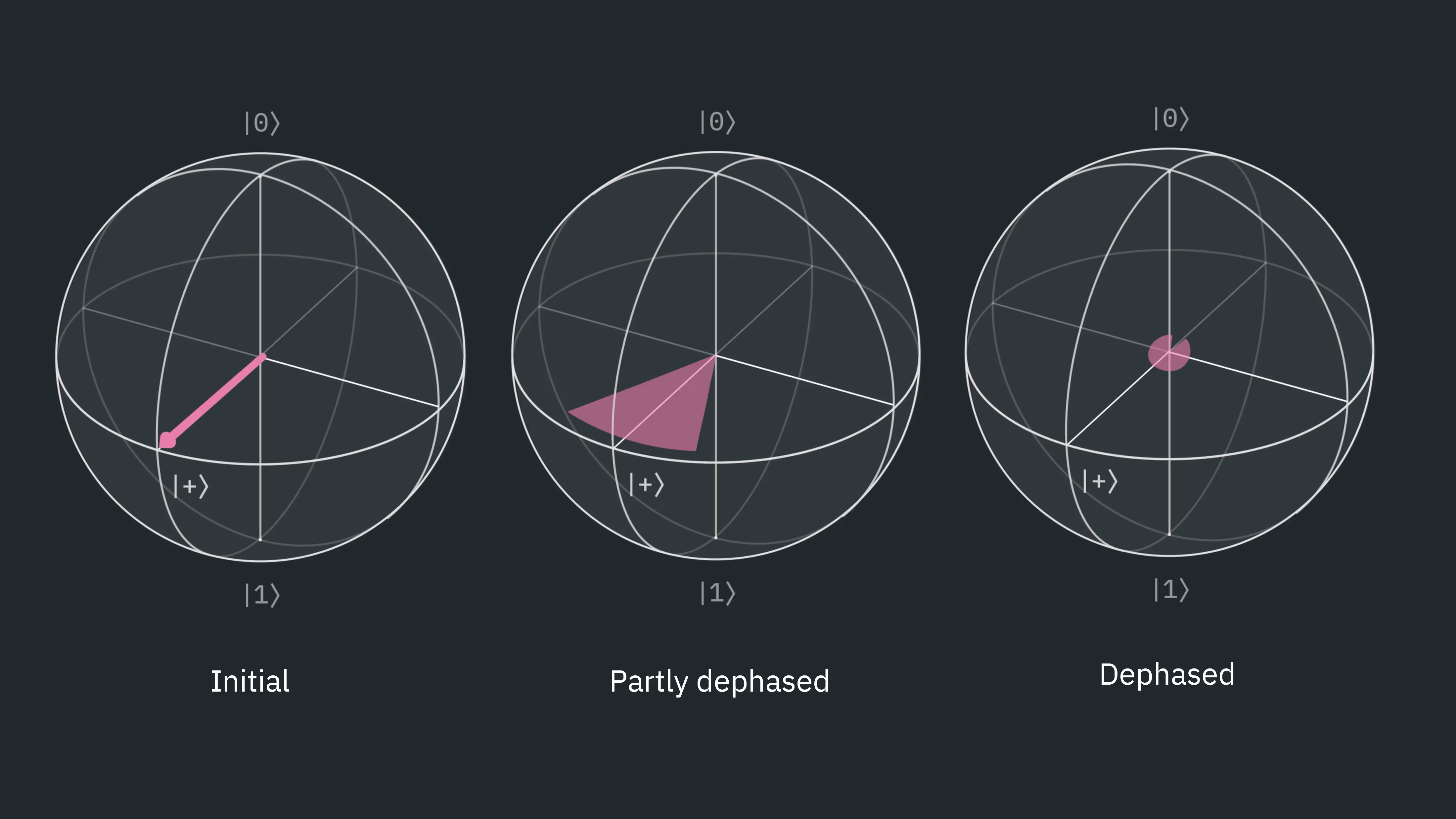
แน่นอนว่าในการทดลองจริง เราไม่มีทางรู้ได้ว่าการเชื่อมโยงแบบสุ่มใดจะเกิดขึ้น แล้วเราจะทำอะไรกับเรื่องนี้ได้บ้าง?

สมมติว่าการเชื่อมโยงกับสภาพแวดล้อมคงที่โดยประมาณตลอดช่วงเวลา $2t_0$ ลองพิจารณาว่าจะเกิดอะไรขึ้นหากเราปฏิบัติตามขั้นตอนต่อไปนี้:

• ปล่อยให้เฟสเปลี่ยนแปลงเป็นเวลา $t_0$

• ใช้ X gate กับ qubit

• ปล่อยให้การเชื่อมโยงกับสภาพแวดล้อมแบบเดียวกันเกิดขึ้นต่ออีกเป็นเวลา $t_0$

• ใช้ X gate ตัวที่สอง

หลังจากวิวัฒนาการตามเวลาในช่วงแรก เราจะได้สถานะข้างต้นพอดี เมื่อใช้ X gate ตัวแรก เราจะได้:

$$X|\psi(t_0)\rangle = \frac{1}{\sqrt{2}}\left( e^{-i\omega_B t_0/2}|1\rangle +e^{i\omega_B t_0/2}|0\rangle \right)$$

เมื่อช่วงเวลา $t_0$ ที่สองผ่านไป ปฏิสัมพันธ์แบบเดียวกันก็เกิดขึ้นอีกครั้ง แต่คราวนี้แอมพลิจูดเชื่อมโยงกับ Z eigenstate ที่ตรงข้ามกัน หมายความว่าเครื่องหมายของการหมุนรอบแกน Z ได้สลับกัน หลังจากปล่อยให้ระบบวิวัฒนาการตามเวลาต่ออีก $t_0$ เราจะได้สถานะ:

$$e^{-iZ\omega_B (t-t_0)/2}\frac{1}{\sqrt{2}}\left( e^{-i\omega_B t_0/2}|1\rangle +e^{i\omega_B t_0/2}|0\rangle \right) =\frac{1}{\sqrt{2}}\left( e^{-i\omega_B (t-t_0)/2}e^{i\omega_B t_0/2}|1\rangle +e^{i\omega_B (t-t_0)/2}e^{-i\omega_B t_0/2}|0\rangle \right)$$

และเมื่อแทนค่า $t = 2t_0$ เราจะได้:

$$|\psi(2t_0)\rangle=\frac{1}{\sqrt{2}}\left(|1\rangle +|0\rangle \right)$$

การใช้ X gate ตัวสุดท้ายไม่มีผลใด ๆ ในกรณีนี้ แต่โดยทั่วไปแล้วจำเป็นต้องใช้:

$$|\psi(2t_0)\rangle = \frac{1}{\sqrt{2}}\left(|0\rangle +|1\rangle \right) = |\psi(t=0)\rangle$$

เราได้กู้คืนสถานะควอนตัมดั้งเดิม รวมถึงเฟสสัมพัทธ์ของมันด้วย กระบวนการนี้เป็นตัวอย่างที่เรียบง่ายเป็นพิเศษของ dynamical decoupling

โดยทั่วไปแล้ว dynamical decoupling (DD) เกี่ยวข้องกับการแทรก single-qubit gate บางตัวเพื่อลดผลกระทบของปฏิสัมพันธ์กับระบบภายนอก qubit (การแยก qubit ออกจากสภาพแวดล้อม) การรวมประวัติเฟสที่เป็นไปได้ทั้งหมดกลับสู่สถานะดั้งเดิมอย่างสมบูรณ์ ดังที่แสดงข้างต้น เป็นสถานการณ์ที่ค่อนข้างอุดมคติ แต่ก็ยังเป็นสถานการณ์ที่เป็นไปได้ มาพูดคุยกันว่า DD มีประโยชน์เมื่อใด และมีข้อควรระวังอะไรบ้าง

ตรวจสอบความเข้าใจของคุณ

ในเนื้อหาข้างต้น เราได้แสดงขั้นตอนผลของลำดับ DD แบบ XX ต่อสถานะเริ่มต้น $|+\rangle$ ลองตรวจสอบว่าขั้นตอนเดียวกันข้างต้นสามารถทำให้สถานะ $|+i\rangle$ กลับคืนสู่สถานะเริ่มต้นได้หรือไม่ ภายใต้สมมติฐานเดียวกันของสนามแม่เหล็กที่เปลี่ยนแปลงอย่างช้า ๆ ตามแนวแกน z

คำตอบ

$$|\psi(t)\rangle = e^{-iZ\omega_B t/2}\frac{1}{\sqrt{2}}\left( |0\rangle +i|1\rangle \right) =\frac{1}{\sqrt{2}}\left( e^{-i\omega_B t/2}|0\rangle +i e^{i\omega_B t/2}|1\rangle \right)$$

หลังจากวิวัฒนาการตามเวลาในช่วงแรก เราจะได้สถานะข้างต้นพอดี เมื่อใช้ X gate ตัวแรก เราจะได้:

$$X|\psi(t_0)\rangle = \frac{1}{\sqrt{2}}\left( e^{-i\omega_B t_0/2}|1\rangle +i e^{i\omega_B t_0/2}|0\rangle \right)$$

เมื่อช่วงเวลา $t_0$ ที่สองผ่านไป ปฏิสัมพันธ์แบบเดียวกันก็เกิดขึ้นอีกครั้ง แต่คราวนี้แอมพลิจูดเชื่อมโยงกับ Z eigenstate ที่ตรงข้ามกัน หมายความว่าเครื่องหมายของการหมุนรอบแกน Z ได้สลับกัน หลังจากปล่อยให้ระบบวิวัฒนาการตามเวลาต่ออีก $t_0$ เราจะได้สถานะ:

$$e^{-iZ\omega_B (t-t_0)/2}\frac{1}{\sqrt{2}}\left( e^{-i\omega_B t_0/2}|1\rangle +i e^{i\omega_B t_0/2}|0\rangle \right) =\frac{1}{\sqrt{2}}\left( e^{-i\omega_B (t-t_0)/2}e^{i\omega_B t_0/2}|1\rangle +i e^{i\omega_B (t-t_0)/2}e^{-i\omega_B t_0/2}|0\rangle \right)$$

และเมื่อแทนค่า $t = 2t_0$ เราจะได้

$$|\psi(2t_0)\rangle=\frac{1}{\sqrt{2}}\left(|1\rangle +i |0\rangle \right)$$

เมื่อใช้ X gate ตัวสุดท้าย เราจะได้:

$$|\psi(2t_0)\rangle = \frac{1}{\sqrt{2}}\left(|0\rangle +i |1\rangle \right) = |\psi(t=0)\rangle = |+i\rangle$$

เมื่อใดควรใช้ DD

ข้อควรระวังแรกและชัดเจนที่สุดคือเราสมมติว่าเป็น dephasing channel ล้วน ๆ ในการวิเคราะห์ของเรา ปฏิสัมพันธ์ในโลกจริงมักก่อให้เกิดส่วนผสมของ dephasing และกลไกข้อผิดพลาดอื่น ๆ ในการวิเคราะห์ข้างต้น เราเลือกใช้ X gate โดยเฉพาะ ซึ่งเรียกว่าลำดับ XX ใน dynamical decoupling ลำดับนี้เหมาะสำหรับข้อผิดพลาดแบบ dephasing ล้วน ๆ แต่ยังมีลำดับอื่น ๆ ที่อาจนำไปใช้ได้กว้างขวางกว่า เช่น XY4 (แสดงในแผนภาพวงจรด้านล่าง) และ XY8 ที่ซับซ้อนกว่า

ข้อควรระวังอีกประการหนึ่งคือ dynamical decoupling เพิ่ม single-qubit gate ซึ่งอาจเพิ่มข้อผิดพลาดระดับ single-qubit เนื่องจากความไม่สมบูรณ์ของ gate หรือแม้แต่ crosstalk อัตราข้อผิดพลาดของ single-qubit เหล่านี้โดยทั่วไปต่ำกว่าข้อผิดพลาดของ multi-qubit gate มาก ดังนั้นโดยปกติแล้วจึงไม่ใช่ข้อกังวลหลัก แต่ก็เป็นสิ่งที่ควรคำนึงถึงหากมี qubit จำนวนมากที่ใช้ DD หลายครั้งตลอดทั้งวงจรของคุณ

DD มีประโยชน์เมื่อการเชื่อมโยงภายนอกมีเวลาส่งผลต่อสถานะของ qubit เนื่องจาก qubit ถูกแยกออกมาอย่างพิถีพิถัน และการเชื่อมโยงภายนอกควรจะอ่อน สัญญาณรบกวนประเภทนี้จะสังเกตเห็นได้ชัดที่สุดเมื่อ qubit อยู่เฉย ๆ เป็นเวลานาน สำหรับช่วงเวลาว่างสั้น ๆ ผลของ DD อาจเป็นการเพิ่มข้อผิดพลาดของ single-qubit gate ในขณะที่ระงับสัญญาณรบกวนได้เพียงเล็กน้อย ซึ่งอาจทำให้ fidelity ของวงจรของคุณลดลงจริง ๆ

ประเด็นสำคัญ: ใช้ dynamical decoupling เมื่อ qubit อยู่เฉย ๆ เป็นเวลานานเพียงพอ และให้ความสนใจกับประเภทของลำดับ DD ที่ใช้

Dynamical decoupling โดยใช้ Qiskit

ลองสำรวจการใช้ DD โดยพิจารณากรณีของ qubit หลายตัวที่ถูกเตรียมในสถานะ $|+\rangle$ ซึ่งจากนั้นอยู่เฉย ๆ เป็นเวลานาน ในกรณีที่ไม่มีข้อผิดพลาด การเตรียมสถานะหลาย qubit $|\psi\rangle = |+\rangle^{\otimes N}$ แล้วใช้ Hadamard gate ก่อนการวัด (ซึ่งเป็นการวัดใน X basis) ควรให้ผลลัพธ์เป็น 0 เสมอ เมื่อมีสัญญาณรบกวน ผลลัพธ์การวัดจะเป็น 0 เพียงบางส่วนของเวลาเท่านั้น แทนที่จะเป็นความน่าจะเป็น 100% เราคำนวณค่าคาดหวัง X เฉลี่ยจาก qubit หลายตัว นั่นคือ เราสนใจสิ่งต่อไปนี้:

$$f\equiv \frac{1}{N}\sum_{j=0}^{N-1}{\langle\Psi | X_j |\Psi\rangle}$$

โดยที่ $X_j \equiv III..X...II$ ซึ่งตัวดำเนินการ X อยู่ในตำแหน่งที่ $j$ นับจากขวา และ $|\Psi\rangle$ คือสถานะของระบบทั้งหมด

วงจรนี้มีความหน่วงเวลาโดยตั้งใจ ซึ่งค่อนข้างจงใจสำหรับการทำ benchmark อย่างไรก็ตาม เป็นเรื่องปกติมากที่วงจรจริงจะมี qubit ที่อยู่เฉย ๆ ในระหว่างการดำเนินการบางส่วน คุณสามารถคิดว่านี่เป็นแบบจำลองที่ง่ายขึ้นของวงจรที่ซับซ้อนกว่า ซึ่ง qubit บางตัวอยู่เฉย ๆ ในระหว่างการคำนวณบางส่วน การทำ benchmark ประเภทนี้ที่อิงจากวิวัฒนาการของสถานะ $|+\rangle$ มักเรียกว่า Ramsey benchmarking

เราเริ่มต้นด้วยการโหลดแพ็กเกจที่จำเป็นและกำหนดค่าบริการ

# Added by doQumentation — required packages for this notebook
!pip install -q matplotlib numpy qiskit qiskit-aer qiskit-ibm-runtime

# Load key packages

from qiskit_ibm_runtime import QiskitRuntimeService
from qiskit_ibm_runtime import SamplerV2 as Sampler
from qiskit.transpiler.preset_passmanagers import generate_preset_pass_manager
from qiskit import QuantumRegister, ClassicalRegister, QuantumCircuit
import numpy as np

# --------- Configuration ----------

service = QiskitRuntimeService()  # assumes credentials are saved
backend = service.backend("ibm_fez")  # adjust if needed

ตอนนี้เรามากำหนดฟังก์ชันช่วยเหลือบางตัวกัน ก่อนอื่น เราต้องการพูดถึงประเด็นเกี่ยวกับช่วงเวลาว่างที่ยาวนาน คำว่า "ยาวนาน" ในบริบทนี้หมายความว่าอย่างไรกันแน่? เราสามารถรายงานเวลาว่างเป็นไมโครวินาทีได้ง่าย ๆ อย่างไรก็ตาม การรู้ว่ามี two-qubit gate กี่ตัวที่สามารถดำเนินการได้ในช่วงเวลาเดียวกันนั้นมีประโยชน์ สิ่งนี้ทำให้เวลาว่างสะท้อนความลึกของวงจรที่สามารถดำเนินการได้ในช่วงเวลาเดียวกันได้โดยตรงมากขึ้น ฟังก์ชันช่วยเหลือตัวแรกจะดึง two-qubit gate ดั้งเดิมของ backend และกำหนดระยะเวลาของ gate นั้น

ฟังก์ชันที่สองเพียงแค่สร้างวงจร Ramsey (วงจรที่มี qubit อยู่ในสถานะ $|+\rangle$) ใส่ความหน่วงเวลา หมุนโดยใช้ H gate แล้วจึงวัด จำไว้ว่า Hadamard gate (H) แปลง $|+\rangle$ เป็น $|0\rangle$ ดังนั้นการวัด $|0\rangle$ ใน Z basis หลังจาก Hadamard จึงสอดคล้องกับการที่ qubit อยู่ในสถานะ $|+\rangle$ ทันทีก่อนหน้า Hadamard

ฟังก์ชันสุดท้ายของเราแปลงจำนวนนับดิบของผลลัพธ์การวัด 0 และ 1 ให้เป็นค่าคาดหวังของ X

from typing import Tuple
from qiskit.providers import Backend
from numpy.typing import NDArray

# --------- Utilities ----------
def detect_twoq_gate_and_duration(
    backend: Backend, pair: tuple[int, int] = (0, 1)
) -> Tuple[str, float]:
    props = backend.properties()
    candidates = ["cx", "ecr", "cz"]
    for name in candidates:
        try:
            dur = props.gate_length(name, list(pair))
            if dur is not None:
                return name, dur
        except Exception:
            pass
    raise RuntimeError(
        "Could not find a two-qubit gate duration among cx/ecr/cz on this backend."
    )

def make_multiqubit_ramsey_circuit(n: int, delay_dt_ticks: int) -> QuantumCircuit:
    q = QuantumRegister(n, "q")
    c = ClassicalRegister(n, "c")
    qc = QuantumCircuit(q, c)

    qc.h(q)
    qc.barrier()

    for i in range(n):
        qc.delay(delay_dt_ticks, q[i], unit="dt")
    qc.barrier()

    qc.h(q)
    qc.measure(q, c)
    return qc

def counts_to_x_expectations(counts: dict[str, int], n: int) -> NDArray[np.float64]:
    total = sum(counts.values())
    if total == 0:
        return np.zeros(n)

    p0 = np.zeros(n, dtype=float)
    for bitstring, cnt in counts.items():
        bits_rev = bitstring[::-1]
        for i in range(n):
            if bits_rev[i] == "0":
                p0[i] += cnt
    p0 /= total
    return 2.0 * p0 - 1.0

ตอนนี้เราระบุรายละเอียดของการทดสอบของเรา รวมถึงจำนวน qubit และลำดับ gate ที่จะใช้ใน DD (ในกรณีนี้คือ XX) โปรดสังเกตเป็นพิเศษว่าเรากำหนด optimization level เป็นศูนย์ ในทางปฏิบัติ คุณมักจะเลือก optimization level ที่สูงกว่า แต่ในที่นี้เราใช้ level 0 เพื่อให้แน่ใจว่าผลกระทบของข้อผิดพลาดที่ DD มุ่งเป้าไปยังคงมองเห็นได้ สุดท้าย เรากำหนดเวลาลักษณะเฉพาะสำหรับ two-qubit gate บน backend นี้ และพิมพ์เวลาที่เกี่ยวข้องบางส่วน

n_qubits = 10  # number of qubits to test in parallel
shots = 4096
opt_level = 0  # we want to ignore optimization for now
num_steps = 6  # number of delay points
gates_per_step = 20  # "equivalent 2q gates" per step
dd_sequence = "XX"  # "XX" for your request; you might try "XY4" too

# --------- Derive timing: dt and 2q gate time ----------
dt = backend.dt  # seconds per dt
twoq_name, t2q = detect_twoq_gate_and_duration(backend, (0, 1))  # seconds
delay_unit_dt = int(round(t2q / dt))  # dt ticks equivalent to one 2q gate

print(f"Backend: {backend.name}")
print(f"dt = {dt*1e9:.3f} ns per tick")
print(f"Using 2q gate '{twoq_name}' with duration ~ {t2q*1e9:.1f} ns")
print(f"One 2q gate ≈ {delay_unit_dt} dt ticks")

Backend: ibm_fez
dt = 4.000 ns per tick
Using 2q gate 'cz' with duration ~ 68.0 ns
One 2q gate ≈ 17 dt ticks

ตอนนี้เราสร้างวงจรของเราและ transpile สำหรับ backend ที่เราเลือก

# --------- Build circuits for a sweep of delays ----------
pm = generate_preset_pass_manager(optimization_level=opt_level, backend=backend)

equiv_gates_list = [
    j * gates_per_step for j in range(num_steps)
]  # e.g., 0, 100, 200, ...
delay_dt_list = [int(round(delay_unit_dt * m)) for m in equiv_gates_list]
delay_us_list = [(dt * d) * 1e6 for d in delay_dt_list]  # for printing/plotting

circuits = []
for delay_dt in delay_dt_list:
    qc = make_multiqubit_ramsey_circuit(n_qubits, delay_dt)
    qc_isa = pm.run(qc)  # ISA-level scheduling/placement; DD is handled at runtime
    circuits.append(qc_isa)

print("Delay sweep (approx microseconds):", [f"{t:.2f}" for t in delay_us_list])

Delay sweep (approx microseconds): ['0.00', '1.36', '2.72', '4.08', '5.44', '6.80']

เราควรแสดงภาพวงจรอย่างน้อยหนึ่งวงจรเพื่อให้แน่ใจว่าเราได้เขียนโค้ดวงจรของเราด้วยสถานะและความหน่วงเวลาตามที่ต้องการ การแสดงภาพวงจรก่อน transpile qc อาจง่ายกว่า หรือคุณอาจตรวจสอบวงจรที่ transpile แล้ว qc_isa

qc.draw("mpl")

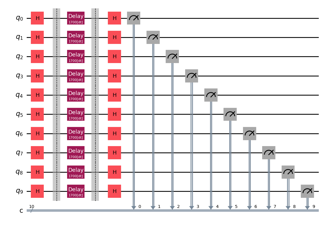
ดำเนินการ

ในที่สุดเราก็พร้อมที่จะดำเนินการบนฮาร์ดแวร์แล้ว เราใช้ Sampler เพื่อรับผลการวัดจำนวนมากของแต่ละ qubit และเราจะใช้มันสองครั้ง: ครั้งหนึ่งโดยปิด DD อย่างชัดเจน และอีกครั้งโดยเปิด DD และใช้ลำดับ gate XX

# --------- Run: NO DD ----------
sampler = Sampler(mode=backend)
sampler.options.default_shots = shots
sampler.options.dynamical_decoupling.enable = False

job = sampler.run(circuits)
res_nodd = job.result()
job_id = job.job_id()  # job id for dd off/false
print("job number for no dd is ", job_id)

# --------- Run: WITH DD (XX) ----------
sampler = Sampler(mode=backend)
sampler.options.default_shots = shots
sampler.options.dynamical_decoupling.enable = True
sampler.options.dynamical_decoupling.sequence_type = (
    dd_sequence  # "XX" first; you can try "XY4" too
)
sampler.options.dynamical_decoupling.scheduling_method = "alap"
sampler.options.dynamical_decoupling.extra_slack_distribution = "middle"

job = sampler.run(circuits)
res_dd = job.result()
job_id = job.job_id()  # job id for dd on/XX
print("job number for dd using XX is ", job_id)

เราสามารถดึงจำนวนนับจากวงจรต่าง ๆ ได้

# --------- Extract counts per circuit ----------

from typing import Iterable, Any

def extract_counts_list(res: Iterable[Any]) -> list[dict[str, int]]:
    counts_list: list[dict[str, int]] = []

    for r in res:  # each r corresponds to one circuit
        counts: dict[str, int] = r.data.c.get_counts()
        counts_list.append(counts)

    return counts_list

counts_list_nodd = extract_counts_list(res_nodd)
counts_list_dd = extract_counts_list(res_dd)

การประมวลผลภายหลัง

ตอนนี้เรามีจำนวนนับจากการวัดแล้ว แต่เราต้องการแปลงให้เป็นค่าคาดหวังของ X แล้วจึงเฉลี่ยค่าคาดหวังเหล่านั้นในทุก qubit ที่เราใช้ เพื่อเรียนรู้เกี่ยวกับการรักษาข้อมูลเฟส สำหรับสิ่งนี้เราใช้ฟังก์ชัน counts_to_x_expectations ที่กำหนดไว้ก่อนหน้านี้

# --------- Compute X-expectations and a scalar contrast ----------
# For each circuit (each delay), compute per-qubit <X> and average absolute contrast.

xexp_nodd = []
xexp_dd = []
contrast_nodd = []
contrast_dd = []

for counts in counts_list_nodd:
    x_vec = counts_to_x_expectations(counts, n_qubits)
    xexp_nodd.append(x_vec)
    contrast_nodd.append(float(np.mean(np.abs(x_vec))))  # average |<X>| across qubits

for counts in counts_list_dd:
    x_vec = counts_to_x_expectations(counts, n_qubits)
    xexp_dd.append(x_vec)
    contrast_dd.append(float(np.mean(np.abs(x_vec))))

# --------- Print a small summary ----------
print("\n=== Summary (average |<X>| per delay) ===")
for m, d_us, c0, c1 in zip(equiv_gates_list, delay_us_list, contrast_nodd, contrast_dd):
    print(
        f"Delay ~ {m:4d} * {twoq_name}  (~{d_us:7.2f} µs):  NoDD={c0: .3f},  DD({dd_sequence})={c1: .3f}"
    )

# Optionally, inspect per-qubit values for the last delay point
print("\nPer-qubit <X> (abs) at the longest delay:")
print("NoDD:", np.round(np.abs(xexp_nodd[-1]), 3))
print("DD  :", np.round(np.abs(xexp_dd[-1]), 3))

=== Summary (average |<X>| per delay) ===
Delay ~    0 * cz  (~   0.00 µs):  NoDD= 0.954,  DD(XX)= 0.961
Delay ~   20 * cz  (~   1.36 µs):  NoDD= 0.827,  DD(XX)= 0.927
Delay ~   40 * cz  (~   2.72 µs):  NoDD= 0.793,  DD(XX)= 0.900
Delay ~   60 * cz  (~   4.08 µs):  NoDD= 0.729,  DD(XX)= 0.876
Delay ~   80 * cz  (~   5.44 µs):  NoDD= 0.661,  DD(XX)= 0.854
Delay ~  100 * cz  (~   6.80 µs):  NoDD= 0.586,  DD(XX)= 0.826

Per-qubit <X> (abs) at the longest delay:
NoDD: [0.05  0.744 0.712 0.867 0.844 0.234 0.473 0.755 0.59  0.587]
DD  : [0.583 0.89  0.921 0.88  0.908 0.832 0.893 0.773 0.807 0.773]

สุดท้าย มาพล็อตผลลัพธ์ของเรากัน

import matplotlib.pyplot as plt

fig, ax = plt.subplots()

# Add values with no DD
ax.scatter(
    equiv_gates_list, contrast_nodd, c="blue", linestyle="-", label="No DD", alpha=0.7
)

## Add values with DD
ax.scatter(
    equiv_gates_list, contrast_dd, c="red", linestyle="-", label="With DD", alpha=0.7
)

# Add labels and plot
ax.set_xlabel("Idle Time in # of 2-qubit gates")
ax.set_ylabel("<X>")
ax.legend()
ax.set_title("Dephasing and DD")
ax.grid(True)

plt.show()

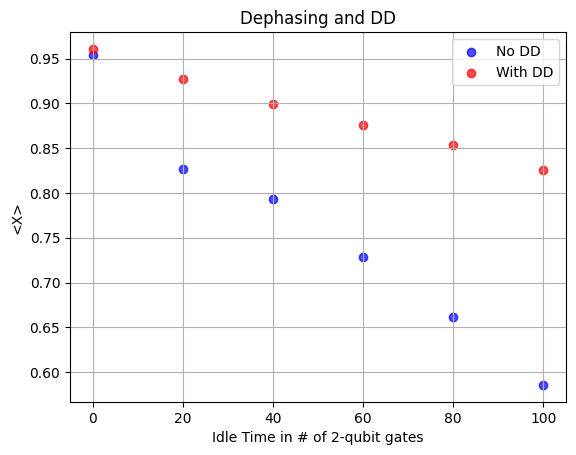
ดังที่คุณเห็น เมื่อไม่มีความหน่วงเวลาอย่างชัดเจน ค่าคาดหวังจะใกล้เคียงกับ 1 จริง ๆ ซึ่งเป็นสิ่งที่เราคาดหวังหากข้อมูลเฟสทั้งหมดถูกรักษาไว้ หากข้อมูลเฟสทั้งหมดสูญหายไป ก็จะไม่มีความโน้มเอียงที่การหมุนครั้งสุดท้ายจะให้ผลลัพธ์เป็น $|0\rangle$ มากกว่า $|1\rangle$ และค่าคาดหวังเฉลี่ยจะเข้าใกล้ศูนย์ ในข้อมูล เราเห็นว่าเมื่อเวลาหน่วงเพิ่มขึ้น ค่าคาดหวังเฉลี่ยของ X จะลดลง เริ่มเข้าใกล้ศูนย์ โปรดสังเกตว่า DD มีประสิทธิภาพมากในที่นี้ ค่าคาดหวังที่มี DD โดยทั่วไปดีกว่า (ใกล้ 1 มากกว่า) มากกว่า 20% เมื่อเทียบกับค่าที่ไม่มี DD แต่ก็ควรสังเกตด้วยว่าจุดข้อมูลที่หน่วงเวลาจุดแรกสอดคล้องกับความหน่วงที่เทียบเท่ากับการดำเนินการ two-qubit gate ประมาณ 100 ครั้ง สิ่งนี้ตอกย้ำประเด็นที่ว่า DD มีประโยชน์มากที่สุดเมื่อ qubit อยู่เฉย ๆ เป็นระยะเวลาที่ค่อนข้างนาน

ตรวจสอบความเข้าใจของคุณ

หากเราใช้ DD ด้วย XY4 กับวงจรเดียวกับก่อนหน้านี้ คุณคาดว่าจะได้ผลลัพธ์ที่ดีกว่ามาก แย่กว่ามาก หรือใกล้เคียงกัน เมื่อเทียบกับ DD ที่ใช้ XX? อธิบาย

คำตอบ

ใกล้เคียงกัน อาจแย่กว่าเล็กน้อย วงจรที่เราใช้มีสถานะที่หมุนเข้าไปในระนาบ XY สถานะนี้เก็บข้อมูลไว้หลัก ๆ ในเฟสของมัน ทำให้มันไวต่อข้อผิดพลาดแบบ dephasing เป็นพิเศษ มากกว่าการคลายตัวแบบ T1 XY4 อาจช่วยเรื่องข้อผิดพลาดที่หลากหลายกว่า แต่ XX ก็ถูกปรับให้เหมาะสมกับวงจรที่เราใช้อยู่แล้ว XY4 อาจดีพอ ๆ กัน แต่จะไม่ได้เพิ่มอะไรที่มีนัยสำคัญ หรือความจริงที่ว่า XY4 มี gate มากกว่าอาจทำให้เกิดข้อผิดพลาดของ gate เพิ่มเติมซึ่งทำให้ผลลัพธ์แย่ลงเล็กน้อย

ผลลัพธ์ล่าสุดใช้ลำดับ DD gate ที่ง่ายที่สุดคือ XX มาดูกันว่าจะทำลำดับที่ซับซ้อนกว่า XY4 ได้อย่างไร เราจะกำหนด Sampler ในส่วนถัดไป

# --------- Run: WITH DD (XY4) ----------
dd_sequence = "XY4"

sampler = Sampler(mode=backend)
sampler.options.default_shots = shots
sampler.options.dynamical_decoupling.enable = True
sampler.options.dynamical_decoupling.sequence_type = dd_sequence
sampler.options.dynamical_decoupling.scheduling_method = "alap"
sampler.options.dynamical_decoupling.extra_slack_distribution = "middle"

job = sampler.run(circuits)
res_xy4 = job.result()
job_id = job.job_id()  # job id for dd on/XY4
print("job number for dd using Xy4 is ", job_id)

job number for dd using Xy4 is  d6k6ti860irc7395d3hg

# --------- Extract counts per circuit ----------

counts_list_xy4 = extract_counts_list(res_xy4)
# --------- Compute X-expectations and a scalar contrast ----------
# For each circuit (each delay), compute per-qubit <X> and average absolute contrast.
xexp_xy4 = []
contrast_xy4 = []

for counts in counts_list_xy4:
    x_vec = counts_to_x_expectations(counts, n_qubits)
    xexp_xy4.append(x_vec)
    contrast_xy4.append(float(np.mean(np.abs(x_vec))))  # average |<X>| across qubits

# --------- Print a small summary ----------
print("\n=== Summary (average |<X>| per delay) ===")
for m, d_us, c0, c1, c2 in zip(
    equiv_gates_list, delay_us_list, contrast_nodd, contrast_dd, contrast_xy4
):
    print(
        f"Delay ~ {m:4d} * {twoq_name}  (~{d_us:7.2f} µs):  NoDD={c0: .3f},  DD({dd_sequence})={c1: .3f}"
    )

# Optionally, inspect per-qubit values for the last delay point
print("\nPer-qubit <X> (abs) at the longest delay:")
print("NoDD:", np.round(np.abs(xexp_nodd[-1]), 3))
print("DD XX :", np.round(np.abs(xexp_dd[-1]), 3))
print("DD XY4 :", np.round(np.abs(xexp_xy4[-1]), 3))

=== Summary (average |<X>| per delay) ===
Delay ~    0 * cz  (~   0.00 µs):  NoDD= 0.968,  DD(XY4)= 0.968
Delay ~  100 * cz  (~   6.80 µs):  NoDD= 0.612,  DD(XY4)= 0.839
Delay ~  200 * cz  (~  13.60 µs):  NoDD= 0.462,  DD(XY4)= 0.705
Delay ~  300 * cz  (~  20.40 µs):  NoDD= 0.339,  DD(XY4)= 0.580
Delay ~  400 * cz  (~  27.20 µs):  NoDD= 0.225,  DD(XY4)= 0.481
Delay ~  500 * cz  (~  34.00 µs):  NoDD= 0.204,  DD(XY4)= 0.393

Per-qubit <X> (abs) at the longest delay:
NoDD: [0.002 0.208 0.447 0.034 0.286 0.306 0.322 0.044 0.163 0.232]
DD XX : [0.433 0.669 0.526 0.516 0.572 0.284 0.303 0.055 0.365 0.208]
DD XY4 : [0.38  0.662 0.521 0.538 0.621 0.252 0.353 0.038 0.239 0.073]

import matplotlib.pyplot as plt

fig, ax = plt.subplots()

# Add values with no DD
ax.scatter(
    equiv_gates_list, contrast_nodd, c="blue", linestyle="-", label="No DD", alpha=0.7
)

## Add values with DD using XX sequence
ax.scatter(
    equiv_gates_list, contrast_dd, c="red", linestyle="-", label="With XX", alpha=0.7
)

## Add values with DD using XY4 sequence
ax.scatter(
    equiv_gates_list,
    contrast_xy4,
    c="black",
    linestyle="-",
    label="With XY4",
    alpha=0.7,
)

# Add labels and plot
ax.set_xlabel("Idle Time in # of 2-qubit gates")
ax.set_ylabel("<X>_av")
ax.legend()
ax.set_title("Dephasing and DD")
ax.grid(True)

plt.show()

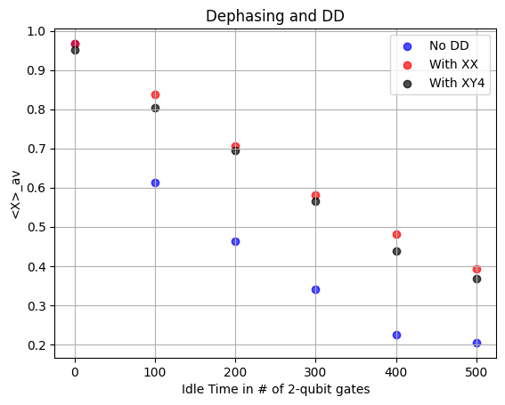
ในที่นี้เราเห็นว่า XY4 ไม่แตกต่างจาก XX อย่างมีนัยสำคัญ มันอาจแย่กว่าเล็กน้อยมากเนื่องจาก gate เพิ่มเติมในลำดับ XY4 แต่ที่สำคัญกว่านั้น เราได้อธิบายไปแล้วว่าทำไม XX จึงให้ผลลัพธ์ตามที่ต้องการในการรักษาเฟสโดยเฉพาะสำหรับสถานะอย่าง $|+\rangle$ ไม่มีเหตุผลที่จะคิดว่าสำหรับสถานะเริ่มต้นเช่นนี้ ลำดับที่แตกต่างกันจะทำให้ผลลัพธ์ดีขึ้น

ตรวจสอบความเข้าใจของคุณ

ตรวจสอบว่าลำดับ XY4 ทำให้สถานะไม่เปลี่ยนแปลง ยกเว้นเฟสรวม (global phase)

คำตอบ

$$\begin{aligned} YXYX|+\rangle & = YXYX(|0\rangle+|1\rangle)\\ & = YXY(|0\rangle+|1\rangle)\\ & = YX(i|1\rangle-i|0\rangle)\\ & = Y(i|0\rangle-i|1\rangle)\\ & = (-|0\rangle-|1\rangle)\\ & =-|+\rangle \end{aligned}$$

Pauli twirling

เราควรเริ่มต้นด้วยการสังเกตว่า Pauli twirling มักถูกใช้ไม่ใช่ในฐานะเทคนิคการระงับข้อผิดพลาด แต่เป็นเทคนิคการปรับรูปข้อผิดพลาด: มันทำให้สัญญาณรบกวน/ข้อผิดพลาดมีพฤติกรรมที่แตกต่างออกไป บางครั้งก็คาดเดาได้ง่ายขึ้น เพื่อให้วิธีการอื่น ๆ สามารถทำงานได้ แม้ว่า Pauli twirling จะไม่ ป้องกัน ข้อผิดพลาด แต่ก็อาจป้องกันการสะสมแบบ coherent ของข้อผิดพลาดได้

ในวงจรควอนตัม แหล่งที่มาของข้อผิดพลาดที่แตกต่างกันหลายแหล่งรวมกัน ข้อผิดพลาดสามารถรวมกันได้หลายวิธี โดยเฉพาะอย่างยิ่งแบบ coherent และ incoherent การสะสมข้อผิดพลาดแบบ coherent หมายความว่าสัญญาณรบกวนหรือการดำเนินการที่ไม่สมบูรณ์มีแนวโน้มที่จะขับเคลื่อนข้อผิดพลาดไปในทิศทางเดียวกันในหลายเลเยอร์และ gate ตัวอย่างหนึ่งคือการหมุนเกิน (over-rotation) แบบ coherent เมื่อใช้ rotation gate

ลองพิจารณา rotation gate ที่สมบูรณ์แบบ เช่น $R_x(\theta_0)$ ซึ่งหมุนรอบแกน X ด้วยมุม $\theta_0$ พอดี แน่นอนว่าการดำเนินการ gate ไม่สมบูรณ์แบบ และการหมุนจริงอาจเป็น $\theta_0+\Delta\theta$ สำหรับการดำเนินการหนึ่งครั้ง และอาจเป็นไปได้ด้วยว่า $\Delta\theta$ มีเครื่องหมายเดียวกันเสมอ และอาจมีขนาดใกล้เคียงกันในหลาย ๆ ครั้งของการใช้ $R_x(\theta)$ ดังนั้น การใช้ rotation gate ซ้ำ ๆ จึงอาจส่งผลให้เกิดการสะสมแบบ coherent ของการหมุนเกิน (หรือหมุนไม่ถึง) จำนวนมากเหล่านี้ $\Delta \theta$

การสะสมข้อผิดพลาดแบบ incoherent ตรงข้ามกันโดยสิ้นเชิง: ข้อผิดพลาดในทิศทางสุ่มด้วยเครื่องหมายสุ่ม ทำให้ข้อผิดพลาดในเลเยอร์ที่แตกต่างกันไม่ได้รบกวนกันแบบบวกกันเสมอไป แต่บางครั้งก็หักล้างกันหรือรวมกันแบบ quadrature เห็นได้ชัดว่าข้อผิดพลาดแบบ incoherent สะสมช้ากว่าในแง่ของผลกระทบโดยรวมต่อสถานะของ qubit แผนภาพจำลองของสิ่งนี้แสดงอยู่ในรูปด้านล่าง นี่เป็นการทำให้เข้าใจง่ายขึ้น ข้อผิดพลาดควอนตัมจริงไม่ได้จำกัดอยู่แค่พื้นที่คาร์ทีเซียนสองมิติ ไม่ใช่ทุกส่วนของข้อผิดพลาดที่มีขนาดเท่ากัน และยังมีความซับซ้อนมากกว่านี้ แต่สัญชาตญาณของภาพแบบนี้มีประโยชน์: ข้อผิดพลาดแบบ coherent มีแนวโน้มที่จะสะสมเร็วกว่าแบบ incoherent

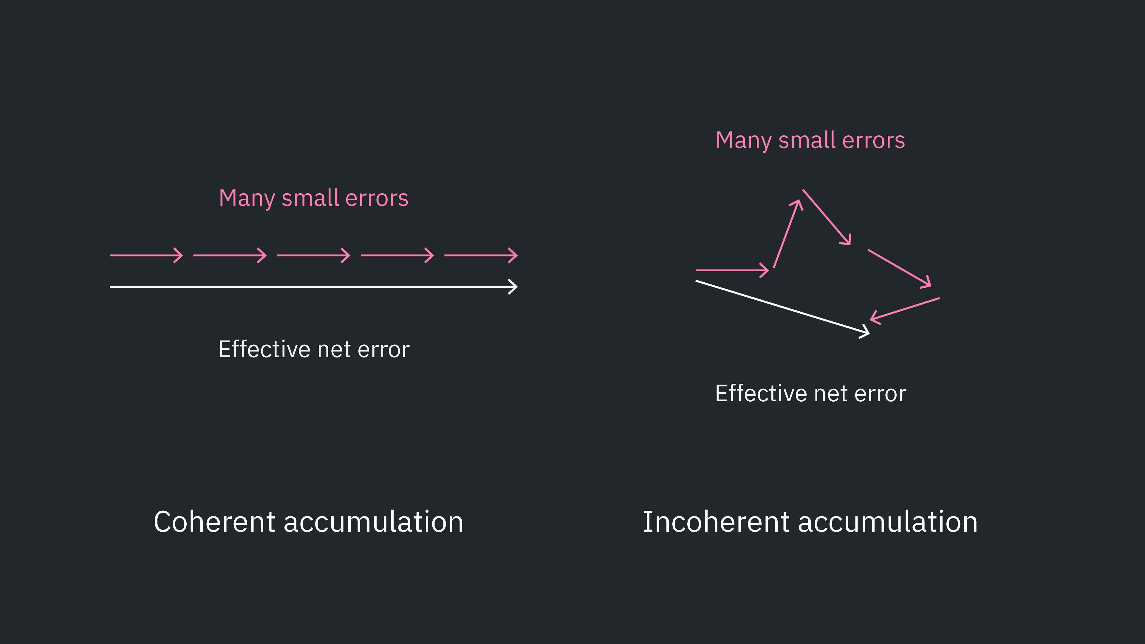
เรามักจะได้ผลลัพธ์ที่มี fidelity สูงขึ้นได้ โดยการเปลี่ยนการสะสมข้อผิดพลาดแบบ coherent ให้เป็นการสะสมข้อผิดพลาดแบบ incoherent วิธีหลักในการทำเช่นนี้เรียกว่า Pauli twirling

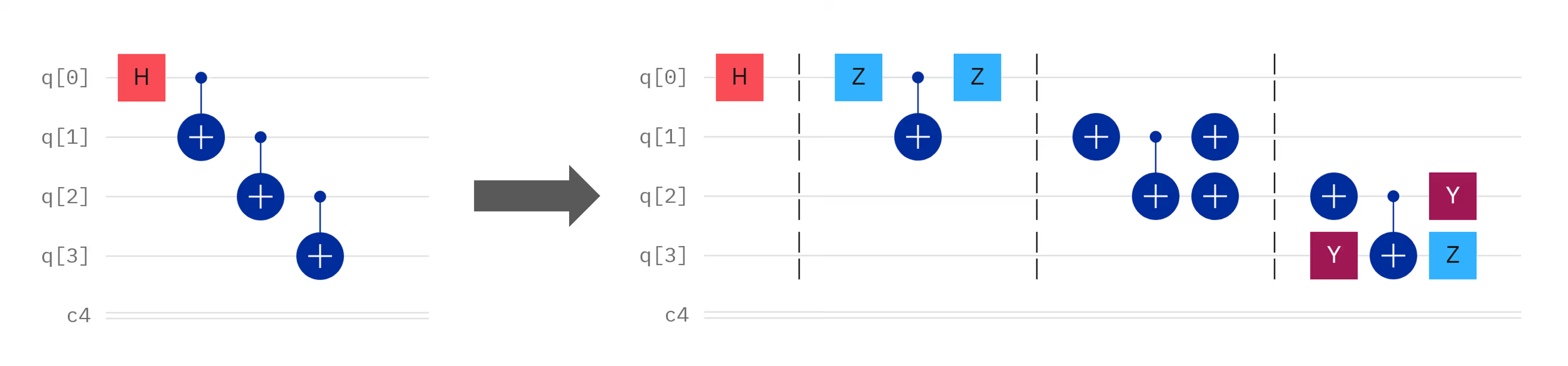
Pauli twirling หมายถึงการเพิ่มชุดผสมของ Pauli gate $P \in \{X, Y, Z, I\}$ ก่อนและหลังการดำเนินการ gate ที่ต้องการ $U$ ในลักษณะที่ $P_1 U P_2 = U$ ในที่นี้ $P_1$ และ $P_2$ ไม่ใช่ Pauli เดี่ยว ๆ แต่เป็นชุดของตัวดำเนินการ Pauli ที่มักจะกระทำกับหลาย qubit บางครั้งคุณอาจเห็นข้อความระบุว่าการกระทำของ Pauli gate เพิ่มเติม "เทียบเท่ากับ identity" แต่นี่ไม่แม่นยำและอาจทำให้สับสนได้ Pauli gate ถูกคั่นด้วย $U$ และเป้าหมายคือการทำให้การกระทำเชิงตรรกะของ gate ทั้งหมดเท่ากับ $U$ บางครั้ง $U$ ถูกเรียกว่า "payload" เพื่อแยกความแตกต่างระหว่างการดำเนินการที่ตั้งใจนี้กับ gate ที่เพิ่มเข้ามาเพื่อการระงับ ตัวอย่างบางส่วนของ Pauli twirling รอบ CNOT gate แสดงอยู่ด้านล่าง

มาดูตัวอย่างเดียวเพื่อตรวจสอบว่า twirling ทำให้ผลกระทบเชิงตรรกะของ payload ไม่เปลี่ยนแปลง โดยไม่สูญเสียความเป็นทั่วไป ให้สถานะสอง qubit ที่เกี่ยวข้องกับ $q_0$ และ $q_1$ เป็น:

$$|\psi_\text{init}\rangle = a|00\rangle + b|01\rangle + c|10\rangle + d|11\rangle$$

เช่นเคย เราใช้ข้อตกลงการเรียงลำดับ qubit $|q_1,q_0\rangle$ เมื่อใช้ CX gate โดยมี $q_1$ เป็นเป้าหมาย จะได้

$$CX|\psi_\text{init}\rangle = |\psi_\text{final}\rangle = a|00\rangle + b|11\rangle + c|10\rangle + d|01\rangle$$

ตอนนี้ลองพิจารณาวงจรที่สามที่แสดง ซึ่งใช้ X gate สำหรับ Pauli twirling เราสามารถคูณเมทริกซ์เข้าด้วยกันแล้วตรวจสอบว่าให้เมทริกซ์ CNOT หรือไม่ อีกทางหนึ่ง เราสามารถติดตามการดำเนินการบนสถานะควอนตัมใด ๆ ผ่านวงจร ดังที่เราทำด้านล่างนี้ สถานะที่จุดต่าง ๆ ในวงจรถูกกำกับด้วยป้าย a-d

$$|\psi_a\rangle = a|00\rangle + b|01\rangle + c|10\rangle + d|11\rangle\\ |\psi_b\rangle = a|01\rangle + b|00\rangle + c|11\rangle + d|10\rangle\\ |\psi_c\rangle = a|11\rangle + b|00\rangle + c|01\rangle + d|10\rangle\\ |\psi_d\rangle = a|00\rangle + b|11\rangle + c|10\rangle + d|01\rangle$$

นี่คือ $|\psi_\text{final}\rangle$ เดียวกันเป๊ะกับที่เราได้มาก่อนหน้านี้โดยไม่มี twirling แท้จริงแล้ว ลำดับ gate ที่ผ่าน twirling นี้ทำให้การกระทำเชิงตรรกะของ payload ไม่เปลี่ยนแปลง อย่างไรก็ตาม หากมีการเลือกลำดับ twirling ที่ถูกต้องแตกต่างกันแบบสุ่มจากเลเยอร์หนึ่งไปอีกเลเยอร์หนึ่ง การสะสมข้อผิดพลาดแบบ coherent สามารถถูกแปลงเป็นการสะสมข้อผิดพลาดแบบสุ่ม (incoherent) ได้อย่างมีประสิทธิภาพ เพื่อความชัดเจน เราไม่ได้เลือกรูปแบบ twirling รูปแบบเดียวแล้วใช้ตลอดทั้งวงจร แต่จะเลือกลำดับ twirling ที่ถูกต้องแตกต่างกันสำหรับแต่ละเลเยอร์ ตัวอย่างที่มีเลเยอร์ entangling จำนวนมากอาจมีลักษณะดังนี้

ตรวจสอบความเข้าใจของคุณ

ตรวจสอบว่า Pauli twirling ในแผงที่สี่ของรูปด้านบนก็ทำให้ผลกระทบเชิงตรรกะของ CNOT ไม่เปลี่ยนแปลงเช่นกัน

คำตอบ

เราจะทำตามตัวอย่างข้างต้นและแสดงให้เห็นว่าการกระทำบนสถานะสอง qubit ใด ๆ เทียบเท่ากับการดำเนินการ CNOT เราจะอ้างอิงถึงจุดที่กำกับไว้ในแผนภาพนี้

$$\begin{aligned} |\psi_a\rangle & = a|00\rangle + b|01\rangle + c|10\rangle + d|11\rangle\\ |\psi_b\rangle & = ai|11\rangle + bi|10\rangle - ci|01\rangle - di|00\rangle\\ |\psi_c\rangle & = ai|01\rangle + bi|10\rangle - ci|11\rangle - di|00\rangle\\ |\psi_d\rangle & = ai(+1)(-i)|00\rangle + bi(-1)(i)|11\rangle - ci(-1)(-i)|10\rangle - di(+1)(i)|01\rangle\\ |\psi_d\rangle & = a|00\rangle + b|11\rangle + c|10\rangle + d|01\rangle \end{aligned}$$

นี่เทียบเท่ากับการกระทำของ CNOT โดยมี qubit 0 เป็น control และ qubit 1 เป็น target

คุณสามารถคิดลำดับ Pauli twirling สำหรับ CNOT gate ที่ไม่ได้แสดงไว้ข้างต้นได้หรือไม่?

คำตอบ

ได้ มีอีกหลายแบบ ตัวอย่างหนึ่งคือ $Z_t$ ก่อน CNOT และ $Z_t$ กับ $Z_c$ หลัง CNOT

เมื่อใดควรใช้ Pauli twirling

ตามที่นำเสนอในที่นี้ Pauli twirling ถูกใช้กับ multi-qubit gate เท่านั้น การใช้โพรโทคอลที่คล้ายกันกับ single-qubit gate จะต้องใช้ตรรกะที่แตกต่างออกไป และโดยทั่วไปไม่มีประโยชน์ในทางปฏิบัติ Pauli twirling เองก็ใช้ single-qubit gate หลายตัว (Pauli gate) Pauli gate เพิ่มเติมมีแนวโน้มที่จะนำมาซึ่งข้อผิดพลาดมากกว่าที่จะได้รับจากการสุ่มการสะสมข้อผิดพลาดแบบ coherent ใด ๆ อัตราข้อผิดพลาดที่เกี่ยวข้องกับ two-qubit gate นั้นมากกว่าอัตราที่เกี่ยวข้องกับ single-qubit gate มาก นอกจากนี้ single-qubit gate บางตัวยังเป็น non-Clifford ซึ่งไม่สามารถทำ twirl ได้อย่างสมบูรณ์ นี่คือเหตุผลที่ Qiskit มีตัวเลือก Pauli twirling ที่ทำการ twirl รอบ two-qubit gate โดยอัตโนมัติ และไม่ทำรอบ single-qubit gate

สิ่งนี้แฝงอยู่ในรูปด้านบน: Pauli twirling ถูกนำไปใช้รอบ CX gate แต่ไม่ใช่รอบ Hadamard gate

มาดูสองตัวอย่างของ Pauli twirling ในการใช้งานจริงกัน

Pauli twirling เพื่อระงับการสะสมแบบ coherent

เพื่อสังเกตว่า Pauli twirling สามารถเปลี่ยนการสะสมข้อผิดพลาดแบบ coherent ให้เป็นการสะสมแบบ incoherent ที่ช้าลงได้อย่างไร เราต้องการวงจรและ observable ที่ทำหน้าที่เป็น stress test สำหรับข้อผิดพลาดแบบ coherent จุดประสงค์เดียวคือทำให้ข้อผิดพลาดของ two-qubit ที่สะสมแบบ coherent มองเห็นได้ แล้วจึงแสดงให้เห็นว่า Pauli twirling แปลงการสะสมแบบ coherent นั้นให้เป็นการเสื่อมสภาพแบบสุ่ม (stochastic) ได้อย่างไร

CNOT (หรือ CZ) gate เป็นแหล่งที่มาทั่วไปของข้อผิดพลาดแบบ coherent การทดลองที่ง่ายที่สุดที่เราสามารถทำได้ในกรณีนี้คือการเตรียมสถานะเริ่มต้น (เช่น $|+\rangle$) ใช้เลเยอร์ของ CNOT gate ที่จับคู่กัน (โดยใช้ข้อเท็จจริงที่ว่า CNOT สองตัวให้ identity) และตรวจสอบว่าข้อผิดพลาดสะสมอย่างไรเมื่อจำนวนเลเยอร์เพิ่มขึ้น ทั้งแบบมีและไม่มี Pauli twirling

observable ที่เราสนใจคือ $\langle X \rangle$ บน qubit เดี่ยว ซึ่งเราพล็อตเป็นฟังก์ชันของจำนวนครั้งที่ทำซ้ำของคู่ CNOT

# --- Imports ---

import numpy as np
from qiskit import QuantumCircuit
from qiskit.transpiler.preset_passmanagers import generate_preset_pass_manager

from qiskit_ibm_runtime import QiskitRuntimeService
from qiskit_ibm_runtime import SamplerV2 as Sampler

# Build the circuit with CX/CX identity per layer

def identity_cx_pairs(layers: int) -> QuantumCircuit:
    q = QuantumRegister(2, "q")
    c = ClassicalRegister(1, "c")  # we only measure q0
    qc = QuantumCircuit(q, c, name=f"N={layers}")

    # |+> on q0
    qc.h(q[0])

    for _ in range(layers):
        qc.barrier()
        qc.cx(q[0], q[1])
        qc.cx(q[0], q[1])

    # Measure in X basis: H then measure q0

    qc.h(q[0])
    qc.measure(q[0], c[0])

    return qc

เนื่องจากเราหมุน basis ของเราก่อนการวัด การวัด $|0\rangle$ จึงสอดคล้องกับสถานะที่อยู่ใน $|+\rangle$ ก่อนหน้า Hadamard gate ตัวสุดท้าย และเช่นเดียวกันสำหรับ $|1\rangle$ และ $|-\rangle$ ดังนั้น ค่าคาดหวัง $\langle X \rangle$ ของเราสามารถคำนวณได้ง่าย ๆ จากจำนวนนับของ $|0\rangle$ ลบด้วยจำนวนนับของ $|1\rangle$

# Compute <X> from SamplerV2 counts

def x_expect_from_counts(counts: dict[str, int]) -> float:
    shots = sum(counts.values())
    p0 = counts.get("0", 0) / shots
    p1 = counts.get("1", 0) / shots
    return p0 - p1  # <X> = P(0) - P(1) after H,measure

เราเลือกจำนวนเลเยอร์ CNOT ที่เหมาะสมเพื่อให้ข้อผิดพลาดสะสม สร้างวงจรของเรา แล้วจึง transpile

# Choose the number of layers for the experiment
N_layers_list = [0, 1, 2, 3, 4, 5]

circuits = [identity_cx_pairs(n) for n in N_layers_list]

# Transpile to backend ISA so that primitives run native instructions
pm = generate_preset_pass_manager(backend=backend, optimization_level=0)
isa_circuits = [pm.run(c) for c in circuits]

โปรดจำไว้ว่าแต่ละเลเยอร์ประกอบด้วย two-qubit gate มากกว่าหนึ่งตัว ตรวจสอบความลึกของ two-qubit ที่ transpile แล้วโดยใช้ฟังก์ชันด้านล่าง

# We can check the 2-qubit depths of any of our circuits like this:
print(
    "two-qubit depth",
    isa_circuits[5].decompose().depth(lambda instr: len(instr.qubits) > 1),
)

two-qubit depth 15

# Configure two Samplers: (A) no twirling, (B) gate twirling
#    - No DD, no measurement twirling in both (to isolate gate twirling)
# ------------------------------
shots = 8192

# (A) No twirling
sampler_no_twirl = Sampler(mode=backend)
# Ensure no extra suppression/mitigation:
sampler_no_twirl.options.dynamical_decoupling.enable = False
# Be explicit about twirling:
sampler_no_twirl.options.twirling.enable_gates = False
sampler_no_twirl.options.twirling.enable_measure = (
    False  # TREX-style measurement twirling off
)
sampler_no_twirl.options.default_shots = shots  # default shots for this primitive

# (B) Gate twirling ON
sampler_twirl = Sampler(mode=backend)
sampler_twirl.options.dynamical_decoupling.enable = False
sampler_twirl.options.twirling.enable_gates = True  # <-- enable Pauli gate twirling
sampler_twirl.options.twirling.enable_measure = False
sampler_twirl.options.default_shots = shots

# (Optional) Inspect options dicts if you’re curious
# print(asdict(sampler_no_twirl.options))
# print(asdict(sampler_twirl.options))

ตอนนี้เรารัน job

# Run both jobs; extract counts; compute <X>

# Helper to run a sampler and compute <X> per circuit
def run_and_x_expect(sampler: Sampler, circ_list: list[QuantumCircuit]) -> list[float]:
    job = sampler.run(
        circ_list
    )  # shots taken from options.default_shots unless overridden
    result = job.result()
    # For SamplerV2, use join_data().get_counts() to combine registers if needed
    exp_vals = []
    for pub in result:
        counts = pub.join_data().get_counts()
        exp_vals.append(x_expect_from_counts(counts))
    return exp_vals

x_no_twirl = run_and_x_expect(sampler_no_twirl, isa_circuits)
x_twirl = run_and_x_expect(sampler_twirl, isa_circuits)

# ------------------------------
# 6) Print a small table
# ------------------------------
print("\nN_layers   <X> (no twirl)   <X> (gate twirl)")
for n, a, b in zip(N_layers_list, x_no_twirl, x_twirl):
    print(f"{n:7d}   {a:14.6f}   {b:14.6f}")

N_layers   <X> (no twirl)   <X> (gate twirl)
      0         0.984375         0.987549
      1         0.934326         0.936523
      2         0.844238         0.892822
      3         0.712158         0.879395
      4         0.592529         0.844971
      5         0.449463         0.785156

สุดท้าย เราแสดงภาพผลลัพธ์เหล่านี้

import matplotlib.pyplot as plt

fig, ax = plt.subplots()

# Add values using XX
ax.scatter(
    N_layers_list, x_no_twirl, c="blue", linestyle="-", label="No twirl", alpha=0.7
)

## Add values with XY4
ax.scatter(N_layers_list, x_twirl, c="red", linestyle="-", label="Twirled", alpha=0.7)

# Add labels and plot
ax.set_xlabel("CX layers")
ax.set_ylabel("<X>")
ax.legend()
ax.set_title("Pauli twirling")
ax.grid(True)

plt.show()

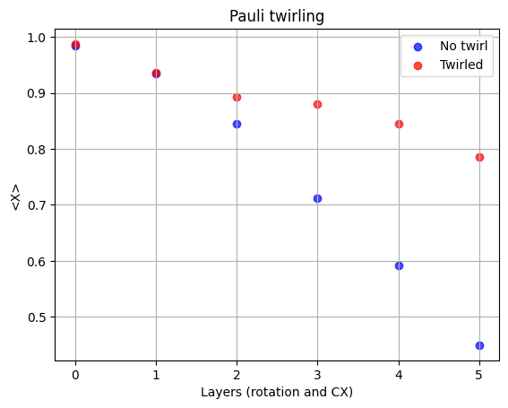
เราสามารถเห็นได้ชัดเจนว่าวงจรที่ผ่าน twirling ให้ค่าคาดหวังที่ใกล้เคียงกับค่าอุดมคติ $\langle X \rangle = 1$ มากกว่า ตัวอย่างนี้ทำหน้าที่ของมันแล้ว แต่มาไปสู่สิ่งที่มีประโยชน์มากขึ้นกันดีกว่า: twirling ในการผลิตสถานะที่พันกันสูง

Pauli twirling ในการเตรียมสถานะ GHZ

ตัวอย่างก่อนหน้านี้แสดงให้เห็นกรณีที่น่าเชื่อถือสำหรับ Pauli twirling ในการทำลายการสะสมแบบ coherent ของข้อผิดพลาดที่เกี่ยวข้องกับ CNOT gate การผลิตสถานะ GHZ ใช้ CNOT gate จำนวนมากเพื่อผลิตสถานะที่พันกันสูงซึ่งมีประโยชน์สำหรับการประยุกต์ใช้ควอนตัมคอมพิวติงหลายอย่าง มาสำรวจกันว่า Pauli twirling ช่วยในบริบทนี้อย่างไร ด้วยสถานะ GHZ ที่มีขนาดเพิ่มขึ้น

# Imports if not already loaded in previous cells
# from qiskit.transpiler.preset_passmanagers import generate_preset_pass_manager
# from qiskit import QuantumRegister, ClassicalRegister, QuantumCircuit

# Define a GHZ circuit building function, so that we can build GHZ states of increasing size.

def ghz_circuit(n: int) -> QuantumCircuit:
    q = QuantumRegister(n, "q")
    c = ClassicalRegister(n, "c")
    qc = QuantumCircuit(q, c)

    qc.h(q[0])
    for i in range(n - 1):
        qc.cx(q[i], q[i + 1])

    qc.barrier()

    qc.measure(q, c)
    return qc

# Build a test state with 10 qubits to remind ourselves of GHZ structure.

num_qubits = 10

qc_ghz = ghz_circuit(num_qubits)
qc_isa = pm.run(qc_ghz)
qc_ghz.draw("mpl")

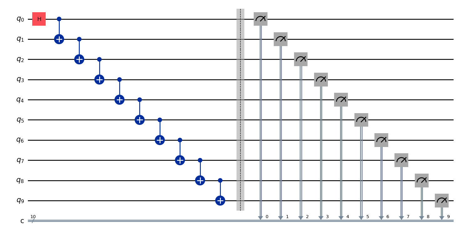
ตอนนี้เราสร้างวงจรของเราและ transpile ในกรณีนี้ เราไม่มี gate ที่ทำซ้ำอย่างประดิษฐ์ที่ลดรูปเป็น identity ดังนั้นเราจึงสามารถให้ pass manager ทำการปรับให้เหมาะสมเพิ่มเติมให้เราได้ เราจะตั้งค่าเป็น level สาม

# Set up a pass manager

opt_level = 3
# --------- Build circuits for a sweep of delays ----------
pm = generate_preset_pass_manager(optimization_level=opt_level, backend=backend)

# Build GHZ circuits of increasing size.

nmin = 5
nmax = 15
circuits = []
for n in range(nmin, nmax):
    qc = ghz_circuit(n)
    qc_isa = pm.run(qc)
    circuits.append(qc_isa)

เราสามารถเห็นได้ว่าตัวปรับให้เหมาะสม (optimizer) แมปวงจรนามธรรมของเราไปยัง qubit 123, 124, 136, 142 และ 143

circuits[0].draw("mpl")

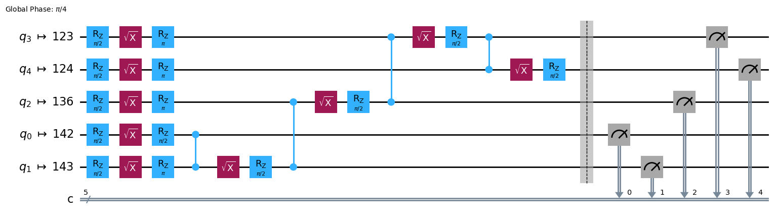
เพื่อทำความเข้าใจว่าทำไม มาดูแผนผังของ backend ของเรา (ในภาพนี้คือ ibm_fez แต่คุณสามารถทำการวิเคราะห์แบบเดียวกันนี้กับ backend ใดก็ได้)

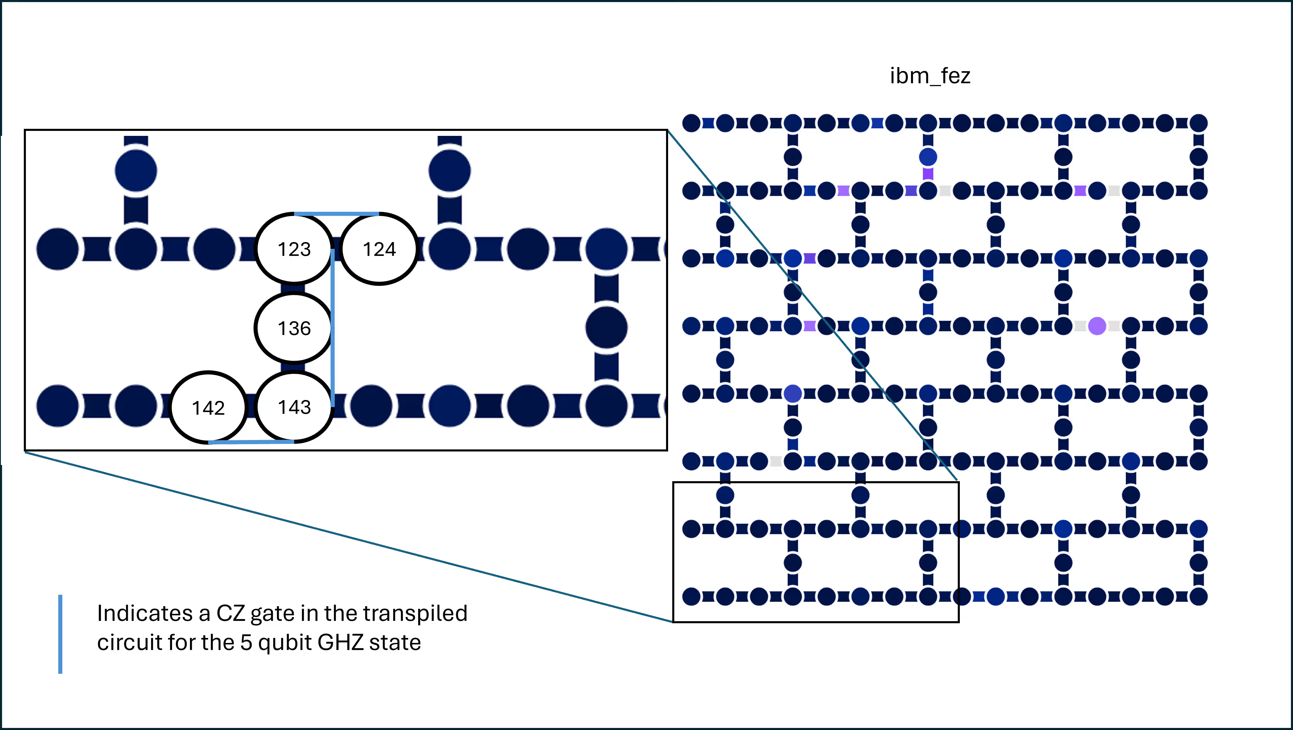
เราเห็นว่า qubit ถูกเลือกเป็นสายโซ่เพื่อลด swap gate ให้น้อยที่สุด และด้วยเหตุนี้จึงลดความลึกของวงจร นอกจากนี้ แต่ละ CZ gate ที่ดำเนินการในวงจรอยู่ระหว่าง qubit ที่อยู่ติดกัน สุดท้าย qubit ทั้งห้าตัวมีอัตราข้อผิดพลาดที่ค่อนข้างต่ำ รวมถึงอัตราข้อผิดพลาดของ readout-assignment คุณสามารถตรวจสอบอัตราข้อผิดพลาดเหล่านี้ได้บน backend ใดก็ได้ในหน้า Compute resources การค้นหาผังงานเช่นนี้ไม่ใช่เรื่องยากสำหรับสายโซ่เชิงเส้นแบบง่าย แต่เมื่อปัญหาซับซ้อนมากขึ้น การปรับให้เหมาะสมของผังวงจรก็จะยากขึ้นและมีคุณค่ามากขึ้น

ตอนนี้เรากำหนดค่า Sampler primitive ของเรา เราปิดเครื่องมือระงับ/บรรเทาข้อผิดพลาดอื่น ๆ เพื่อมุ่งเน้นไปที่ Pauli twirling

# Configure two Samplers: (A) no twirling, (B) gate twirling
# No DD, no measurement twirling in both (to isolate gate twirling)

shots = 8192

# (A) No twirling
sampler_no_twirl = Sampler(mode=backend)
# Ensure no extra suppression/mitigation:
sampler_no_twirl.options.dynamical_decoupling.enable = False
# Be explicit about twirling:
sampler_no_twirl.options.twirling.enable_gates = False
sampler_no_twirl.options.twirling.enable_measure = (
    False  # TREX-style measurement twirling off
)
sampler_no_twirl.options.default_shots = shots  # default shots for this primitive

# (B) Gate twirling ON
sampler_twirl = Sampler(mode=backend)
sampler_twirl.options.dynamical_decoupling.enable = False
sampler_twirl.options.twirling.enable_gates = True  # <-- enable Pauli gate twirling
sampler_twirl.options.twirling.enable_measure = False
sampler_twirl.options.default_shots = shots

# (Optional) Inspect options dicts if you’re curious
# print(asdict(sampler_no_twirl.options))
# print(asdict(sampler_twirl.options))

สุดท้าย เรารัน job ของเรา คุณสามารถเลือกพิมพ์หมายเลข job ID เพื่อเรียกใช้ในภายหลังได้

job = sampler_twirl.run(circuits)
res_ghz_twirl = job.result()
job_id = job.job_id()  # job id for twirling on/true
print("job number for twirling the ghz prep is ", job_id)

job = sampler_no_twirl.run(circuits)
res_ghz_no_twirl = job.result()
job_id = job.job_id()  # job id for twirling off/false
print("job number for NO twirling the ghz prep is ", job_id)

job number for twirling the ghz prep is  d7h967bjne2c7393s0b0
job number for NO twirling the ghz prep is  d7h96f7b91ec73aufing

เราดึงจำนวนนับของแต่ละสถานะฐานเชิงคำนวณที่วัดได้สำหรับทุกวงจร ทั้งแบบมีและไม่มี twirling

# --------- Extract counts per circuit ----------
def extract_counts_list(res):
    counts_list = []
    for r in res:  # each r corresponds to one circuit
        # r.data.<classical_register_name>.get_counts()
        counts = r.data.c.get_counts()
        counts_list.append(counts)
    return counts_list

counts_list_ghz_twirl = extract_counts_list(res_ghz_twirl)
counts_list_ghz_no_twirl = extract_counts_list(res_ghz_no_twirl)

print(counts_list_ghz_twirl[0])
print(counts_list_ghz_twirl[4])

{'11111': 3440, '11101': 87, '00000': 3434, '10111': 87, '00001': 168, '10011': 4, '11000': 102, '00011': 39, '01111': 93, '00111': 111, '01000': 90, '11110': 235, '00110': 6, '00010': 75, '11011': 30, '11100': 42, '10000': 82, '00101': 7, '10001': 2, '11001': 6, '11010': 5, '01010': 3, '01110': 7, '00100': 14, '10101': 1, '10110': 8, '01001': 6, '10100': 1, '01101': 4, '01011': 1, '10010': 2}
{'111111111': 2683, '000000000': 2976, '111000000': 53, '110000000': 74, '111111100': 47, '111011111': 76, '111111110': 195, '111111000': 67, '000000010': 66, '011111110': 10, '011110001': 1, '101110111': 7, '101011111': 9, '111110111': 87, '111100000': 96, '111011000': 2, '010000000': 60, '111111010': 3, '100000000': 110, '111111011': 32, '000000111': 51, '000100000': 84, '000011111': 82, '000000001': 176, '100000010': 6, '111100001': 3, '000000011': 36, '101111111': 98, '100000011': 2, '001111111': 75, '000001000': 60, '000011101': 4, '110111111': 38, '111111101': 72, '111100100': 3, '000100010': 1, '001011101': 1, '000000110': 8, '110000011': 1, '000111111': 48, '000000100': 23, '000001111': 65, '010000101': 2, '000100001': 8, '111110000': 51, '010001111': 1, '111000111': 2, '111000001': 2, '000111100': 1, '011111111': 116, '111110001': 1, '000011110': 10, '000010000': 23, '000101111': 3, '000101110': 1, '011110111': 4, '010000111': 7, '111101111': 36, '001000000': 40, '010100000': 3, '101111110': 8, '110111000': 5, '000000101': 8, '010000010': 4, '000110001': 2, '110111110': 4, '111100010': 2, '111010111': 2, '000001110': 5, '111110101': 3, '001110000': 4, '101100000': 5, '001111110': 8, '100000001': 5, '111011110': 3, '111110100': 5, '110001011': 1, '001110111': 4, '000010110': 2, '111001111': 2, '000011000': 5, '010111110': 1, '000101000': 4, '101000000': 4, '100111111': 4, '111110011': 2, '000101100': 1, '101111100': 2, '111011100': 1, '001111011': 3, '011111011': 3, '110100000': 5, '000001011': 3, '111110110': 5, '111111001': 5, '000001001': 8, '010000001': 5, '011111101': 2, '001010111': 1, '011101110': 1, '110110110': 1, '001111100': 3, '100001000': 3, '001000011': 1, '001011111': 6, '110000010': 2, '110010000': 1, '010011111': 2, '111101101': 3, '101110000': 1, '111100111': 6, '010111111': 5, '110110000': 2, '011011111': 2, '110011111': 1, '110000111': 6, '001000001': 2, '001100000': 3, '101101111': 1, '000111110': 5, '111011101': 2, '100100000': 2, '101111101': 3, '001001111': 1, '001010000': 2, '111001000': 1, '011110000': 2, '011101111': 3, '000001100': 1, '110101000': 1, '011000000': 4, '111101000': 3, '110000001': 4, '000010111': 4, '011111100': 1, '111000010': 1, '101011000': 1, '101111000': 2, '001101111': 1, '010001100': 1, '000100011': 1, '111110010': 1, '111101110': 1, '100001111': 1, '100011011': 1, '010110111': 1, '001110110': 2, '100000100': 1, '001000110': 1, '100011111': 2, '010010001': 1, '111010110': 1, '011110110': 1, '000111000': 2, '000100111': 1, '011010000': 1, '001111000': 2, '100010000': 1, '011111000': 2, '110111100': 2, '110110111': 1, '110001000': 1, '000110111': 1, '000101011': 1, '000110000': 1, '011100000': 3, '001000010': 1, '001001000': 1, '001000111': 1, '001111101': 3, '111101011': 1, '111010000': 1, '100000101': 1, '000010010': 1, '001011110': 1, '000011011': 1, '111101100': 1}

เรารู้ว่าการกระจายตัวในอุดมคติของสถานะ GHZ คือกรณีที่ shot ครึ่งหนึ่งให้ผลลัพธ์ $|0\rangle^{\otimes N}$ และอีกครึ่งหนึ่งให้ผลลัพธ์ $|1\rangle^{\otimes N}$ สร้างสิ่งนี้ขึ้นมาเพื่อเปรียบเทียบ

ideal_dist = []
for n in range(nmin, nmax):
    ideal_dist.append({"0" * n: int(shots / 2), "1" * n: int(shots / 2)})

ตอนนี้เราใช้ Hellinger fidelity เป็นตัววัดคุณภาพของสถานะสุดท้ายของเรา

from qiskit.quantum_info import hellinger_fidelity

num_qubits = []
fidelities_twirl = []
fidelities_no_twirl = []
for n in range(len(ideal_dist)):
    num_qubits.append(nmin + n)
    fidelities_twirl.append(hellinger_fidelity(counts_list_ghz_twirl[n], ideal_dist[n]))
    fidelities_no_twirl.append(
        hellinger_fidelity(counts_list_ghz_no_twirl[n], ideal_dist[n])
    )

สุดท้ายเราพล็อตผลลัพธ์ของเรา

import matplotlib.pyplot as plt

fig, ax = plt.subplots()

# Add values using no twirling
ax.scatter(
    num_qubits,
    fidelities_no_twirl,
    c="blue",
    linestyle="-",
    label="No twirl",
    alpha=0.7,
)

## Add values with twirling
ax.scatter(
    num_qubits, fidelities_twirl, c="red", linestyle="-", label="Twirled", alpha=0.7
)

# Add labels and plot
ax.set_xlabel("Qubits in GHZ state")
ax.set_ylabel("Hellinger fidelity")
ax.legend()
ax.set_title("Pauli twirling in GHZ states")
ax.grid(True)

plt.show()

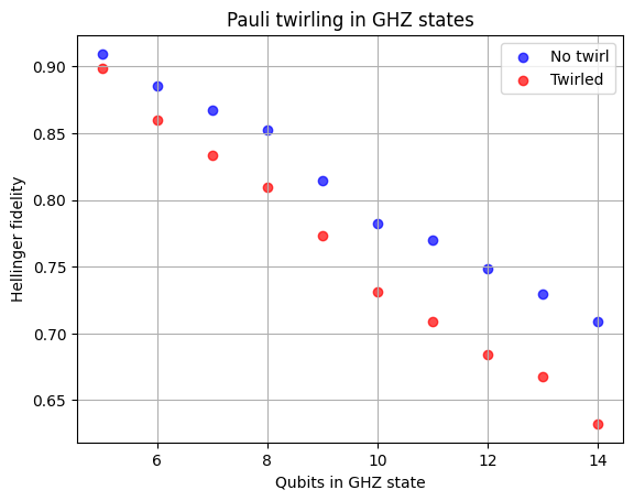
ผลลัพธ์ที่ใช้ Pauli twirling ไม่ได้ดีกว่า (และแม้แต่แย่กว่าเล็กน้อย) เมื่อเทียบกับที่ไม่มี twirling เกิดอะไรขึ้น?

มีสองสิ่งเกิดขึ้น ประการแรก Pauli twirling ไม่ได้ลดปริมาณสัญญาณรบกวนทั้งหมด — แต่จะปรับรูปข้อผิดพลาดที่เป็นระบบและแบบ coherent ให้กลายเป็นข้อผิดพลาดแบบ Pauli ที่เป็นสุ่ม ทำให้การเติบโตของข้อผิดพลาดสามารถคาดเดาได้และสร้างแบบจำลองได้ ไม่เคยมีการรับประกันการลดข้อผิดพลาด ยกเว้นในกรณีพิเศษ

ประการที่สอง ในวงจร GHZ ข้อผิดพลาดแบบ coherent บางส่วนสามารถหักล้างกันบางส่วนหรือทำตัวเหมือนการเลื่อนเฟสที่ไม่เป็นอันตราย เนื่องจากความสมมาตรของโครงสร้าง GHZ twirling ลบการป้องกันโดยบังเอิญนี้ออกไปและแทนที่ด้วยสัญญาณรบกวน Pauli แบบสุ่มที่ไม่มีความสัมพันธ์กัน ทำให้ fidelity ของ GHZ แย่ลงเล็กน้อยภายใต้ twirling

ข้ออ้างที่สองนี้ต้องการคำอธิบายเพิ่มเติม ข้ออ้างนี้ไม่ได้หมายความว่าวงจร GHZ ได้รับการปกป้องจากการสะสมข้อผิดพลาดแบบ coherent ทุก ประเภท แต่เพียงบางประเภทเท่านั้น — และในกรณีเหล่านั้น การป้องกันจะถูกทำลายโดย twirling โดยเฉพาะอย่างยิ่ง ลองพิจารณาการหมุนเกินแบบ coherent ที่เกี่ยวข้องกับ CX gate เรียกชื่อ CX gate จริงที่มีการหมุนเกินว่า $\tilde{CX}$:

$$\tilde{CX}\equiv e^{-i\epsilon K} \cdot CX$$

โดยที่ $K$ คือผลคูณใดๆ ของตัวดำเนินการ Pauli เช่น $X$, $Z$, $Z \otimes X$, $Z^{\otimes N}$ เป็นต้น สำหรับสถานะทั่วไป over-rotation เหล่านี้อาจส่งผลต่อสถิติการวัด (และดังนั้นจึงส่งผลต่อการวัด fidelity ของสถานะ) อย่างไรก็ตาม subset หนึ่งของ over-rotation เหล่านี้ไม่ทำให้ observable มาตรฐานของ GHZ จำนวนมากเปลี่ยนแปลง รวมถึงตัวดำเนินการอย่าง $Z_i Z_j$ และ $Z^{\otimes N}$ ในบริบทของการเตรียมสถานะ GHZ ข้อผิดพลาด over-rotation ประเภทนี้ที่เกี่ยวข้องจะเป็น:

$$\tilde{CX}\equiv e^{-i\epsilon Z_c Z_t} \cdot CX$$

การเตรียมสถานะ GHZ ที่มี $N$ qubit ทั้งหมดจะมีลักษณะดังนี้:

$$|\psi_\text{GHZ}\rangle=\prod_{j=0}^{N-2}{e^{-i\epsilon Z_j Z_{j+1}} \cdot CX_{j,j+1}}H^{\otimes N}|0^{\otimes N}\rangle$$

หลังจากเตรียมสถานะ GHZ แล้ว สถานะที่เป็นอุดมคติคือ:

$$|\text{GHZ}^{\otimes N}\rangle=\frac{1}{\sqrt{2}}\left(|0\dots 0\rangle + |1\dots 1\rangle\right).$$

สถานะนี้เป็น simultaneous eigenstate ของชุดตัวดำเนินการ Pauli ขนาดใหญ่ ซึ่งรวมถึงตัวดำเนินการต่อไปนี้:

$$Z_i Z_j \quad \text{for all } i \neq j,$$

ด้วยค่า eigenvalue $+1$ ผลก็คือตัวดำเนินการในรูป $e^{-i\epsilon Z_i Z_j}$ กระทำต่อสถานะ GHZ เป็นการคูณด้วยตัวประกอบเฟส $e^{-i\epsilon}$ ซึ่งไม่ส่งผลต่อ observable มาตรฐานของ GHZ เช่น parity, $X^{\otimes N}$ แบบรวม หรือ population ใน computational basis ดังนั้น แม้ว่าข้อผิดพลาด over-rotation $e^{-i\epsilon Z_j Z_{j+1}}$ จะเป็น coherent และเป็นระบบ แต่ก็แทบมองไม่เห็นสำหรับการวัดที่ใช้ประเมิน fidelity ของ GHZ ในแง่นี้ วงจร GHZ ได้รับการปกป้องความ coherent โดยบังเอิญ กล่าวคือ ข้อผิดพลาด CX แบบ coherent บางชนิด commute กับโครงสร้างของสถานะที่กำลังเตรียม จึงไม่ทำให้ประสิทธิภาพที่วัดได้ลดลง

Pauli twirling เปลี่ยนแปลงสถานการณ์นี้อย่างพื้นฐาน การ twirl ไม่รักษาข้อผิดพลาด over-rotation แบบ coherent ให้เป็น process $Z_jZ_{j+1}$ แบบ deterministic แต่จะแปลง error channel แบบ coherent ให้กลายเป็น stochastic Pauli channel ที่มีผล ผลก็คือ error channel ตอนนี้มีเทอมอย่าง $X$, $Y$, $X \otimes Z$ และ $Y \otimes X$ ซึ่งไม่ commute กับ stabilizer ของ GHZ

เมื่อข้อผิดพลาด stochastic Pauli เหล่านี้เกิดขึ้น มันสร้าง fault แบบ bit-flip และ phase-flip จริงบน qubit เดี่ยวหรือคู่ qubit ข้อผิดพลาดเหล่านี้นำสถานะออกจาก GHZ stabilizer subspace ลด interference ระหว่าง $|0\dots 0\rangle$ และ $|1\dots 1\rangle$ และลด GHZ fidelity และสัญญาณ parity แบบหลาย qubit โดยตรง กล่าวอีกนัยหนึ่ง Pauli twirling ลบโครงสร้าง coherent ของข้อผิดพลาดออกไป แต่ก็ลบการหักล้างที่อาศัยความสมมาตรซึ่งเคยทำให้ข้อผิดพลาดเหล่านั้นไม่เป็นอันตรายออกไปด้วย ผลลัพธ์คือสถานะ GHZ ที่แย่ลงเล็กน้อย — ไม่ใช่เพราะ twirling เพิ่ม noise แต่เพราะมันแปลงข้อผิดพลาด coherent ที่ส่วนใหญ่ไม่เป็นอันตรายให้กลายเป็นข้อผิดพลาด stochastic ที่สร้างความเสียหายจริง

ตัวอย่างนี้ชี้ให้เห็นบทเรียนสำคัญ: Pauli twirling ไม่ใช่กลยุทธ์ปรับปรุงแบบสากล มันมีประโยชน์มากที่สุดเมื่อข้อผิดพลาด coherent สะสมตลอดวงจรในลักษณะที่ทำลาย fidelity ที่ต้องการ ในวงจรที่มีความสมมาตรสูงอย่างการเตรียมสถานะ GHZ ข้อผิดพลาด coherent บางส่วนสอดคล้องตามธรรมชาติกับ stabilizer ของสถานะ และการสุ่มมันโดยตั้งใจสามารถลบการปกป้องโดยบังเอิญนี้ออกไปได้

รวมวิธีการ

ในหลักการ เราสามารถรวม Pauli twirling เข้ากับ dynamical decoupling ได้ เราไม่ได้ใช้ DD ในกรณีนี้ด้วยเหตุผลสองประการ ประการแรกไม่ควรมีช่วงเวลา idle ที่ยาวมากในวงจรนี้ ประการที่สอง สถานะ GHZ ไม่ได้เก็บข้อมูลส่วนใหญ่ไว้ใน single-qubit phase coherence โดยเฉพาะอย่างยิ่งหากเราสังเกต fidelity เฉพาะในแง่ของ bitstring count ไม่ใช่ในแง่ของเฟสระหว่าง bitstring ที่ต้องการ $|0\rangle^{\otimes N}$ และ $|1\rangle^{\otimes N}$

หากเราขยายการเตรียม GHZ ไปยัง 100+ qubit ความล่าช้าในการวัด qubit แรกๆ/ต้นๆ อาจยาวนานพอที่ DD จะมีประโยชน์จริงๆ โดยเฉพาะอย่างยิ่งเมื่อเราคำนึงถึง transpiled depth ของวงจร

Pauli twirling ในโครงสร้าง RTZ echo

ตัวอย่างสุดท้ายของเราสำหรับ Pauli twirling ในบริบทของการลดการสะสมข้อผิดพลาด coherent ใช้วงจรที่มีชั้นของการรวมกัน X-CZ-X-CZ นี่เป็นลำดับ gate ที่รู้จักกันดีซึ่งมักใช้เพื่อหักล้างเทอมข้อผิดพลาด ZZ แบบ coherent ใน two-qubit gate แม้ไม่มีการ twirl แต่ด้วยการ twirl เราสามารถลดหรือสุ่มรูปแบบอื่นๆ ของการสะสมข้อผิดพลาด coherent ได้

เราจะเริ่มด้วยการกำหนดฟังก์ชันเพื่อสร้างวงจรแบบ RTZ ที่มีจำนวนชั้นแตกต่างกัน

from qiskit import QuantumCircuit

def rtz_echo_circuit(n_qubits: int, depth: int) -> QuantumCircuit:
    """
    Construct an RTZ echo-style circuit.

    Args:
        n_qubits: Number of qubits in the circuit.
        depth: Number of repeated echo layers.

    Returns:
        A QuantumCircuit implementing the echo sequence with measurements.
    """
    q = QuantumRegister(n_qubits, "q")
    c = ClassicalRegister(n_qubits, "c")
    qc = QuantumCircuit(q, c)

    for _ in range(depth):
        qc.h(q)

        for i in range(0, n_qubits - 1, 2):
            qc.cz(q[i], q[i + 1])

        qc.x(q)

        for i in range(1, n_qubits - 1, 2):
            qc.cz(q[i], q[i + 1])

        qc.h(q)

    qc.measure(q, c)
    return qc

ตอนนี้เราสร้างวงจรที่มีจำนวนชั้นเพิ่มขึ้น จนถึง two-qubit depth ที่ transpile แล้วรวมที่สมเหตุสมผล

from qiskit.transpiler.preset_passmanagers import generate_preset_pass_manager

circuits = []
qcs = []
depths = list(range(3, 27, 4))
n_qubits = 10

opt_level = 0
pm = generate_preset_pass_manager(
    optimization_level=opt_level,
    backend=backend,
    initial_layout=[0, 1, 2, 3, 4, 5, 6, 7, 8, 9],
)

for d in depths:
    qc = rtz_echo_circuit(n_qubits, d)
    qcs.append(qc)
    qc_isa = pm.run(qc)
    circuits.append(qc_isa)

# We can check the 2-qubit depths of any of our circuits like this:
two_qubit_depths = []
for n in range(len(circuits)):
    two_qubit_depths.append(
        circuits[n].decompose().depth(lambda instr: len(instr.qubits) > 1)
    )
print(two_qubit_depths)

[6, 14, 22, 30, 38, 46]

qcs[0].draw("mpl")
# circuits[0].draw("mpl")

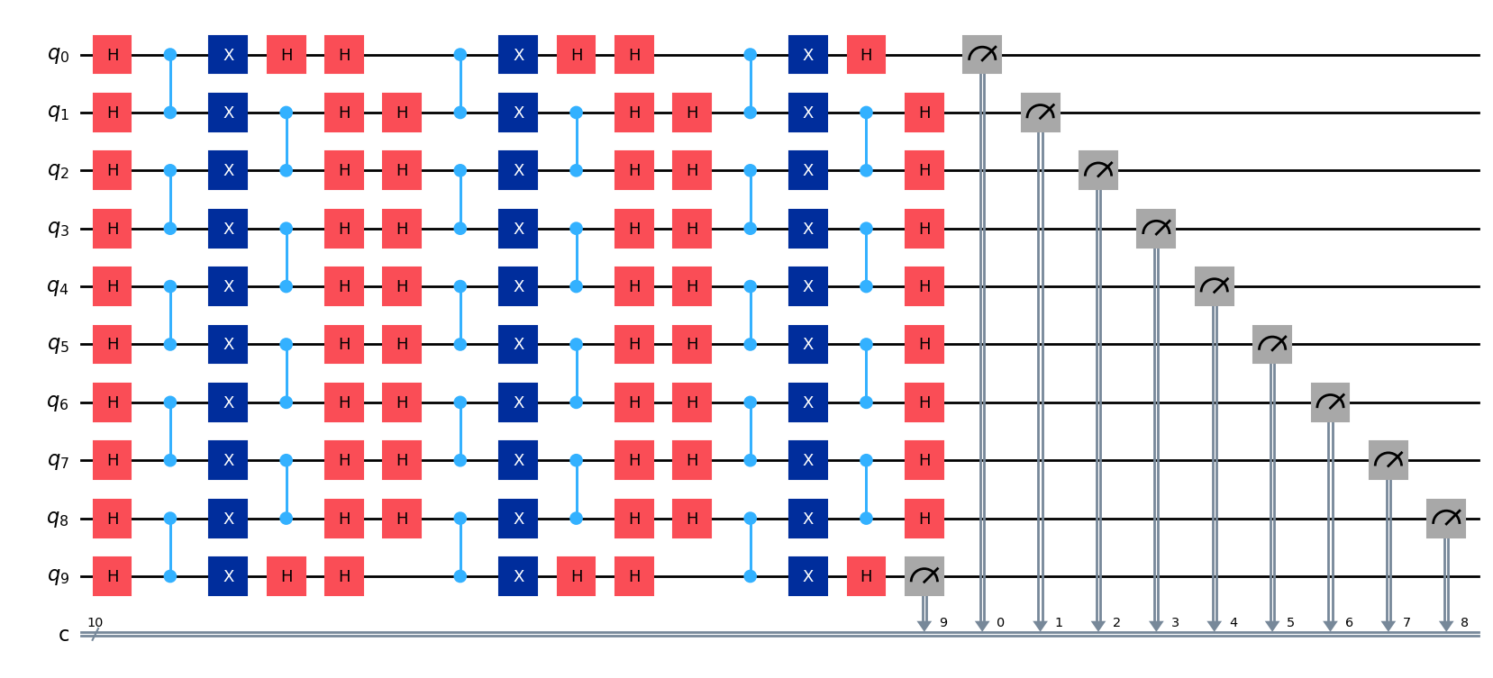
ในระดับสูงสุด บางวงจรเหล่านี้ลึกมาก มาใช้ AerSimulator ที่ไม่มี noise model เพื่อหาสถานะในอุดมคติที่ปลายวงจรแต่ละวงจรกัน จากนั้นเราสามารถ benchmark ผลลัพธ์ของเราจากคอมพิวเตอร์ควอนตัมจริงโดยใช้ Hellinger fidelity

from qiskit_aer import AerSimulator

sim = AerSimulator()
ideal_results = sim.run(circuits, shots=8192).result()
ideal_counts = ideal_results.get_counts()

ตอนนี้เรากำหนด SamplerV2 แบบมีการ twirl และแบบไม่มีการ twirl

from qiskit_ibm_runtime import SamplerV2 as Sampler

shots = 8192

# --- No Twirling ---
sampler_no = Sampler(mode=backend)
sampler_no.options.twirling.enable_gates = False
sampler_no.options.twirling.enable_measure = False
sampler_no.options.default_shots = shots

# --- With Twirling ---
sampler_tw = Sampler(mode=backend)
sampler_tw.options.twirling.enable_gates = True
sampler_tw.options.twirling.enable_measure = False
# sampler_tw.options.twirling.num_randomizations = "auto"
sampler_tw.options.twirling.num_randomizations = 32
sampler_tw.options.twirling.strategy = "active-circuit"
sampler_tw.options.default_shots = shots

ตอนนี้เรารันงานของเรา

# Each job took 17 sec (34 sec total) on ibm_fez. Your times might vary.

job_no = sampler_no.run(circuits)
job_tw = sampler_tw.run(circuits)

res_no = job_no.result()
res_tw = job_tw.result()

เราได้ count จากแต่ละการรันบนคอมพิวเตอร์ควอนตัมจริง

counts_no = [r.data.c.get_counts() for r in res_no]
counts_tw = [r.data.c.get_counts() for r in res_tw]

ตอนนี้เราหา Hellinger fidelity โดยเปรียบเทียบแต่ละการรันเหล่านี้กับผลลัพธ์ AerSimulator ที่ไม่มี noise

from qiskit.quantum_info import hellinger_fidelity

f_no = [hellinger_fidelity(counts_no[i], ideal_counts[i]) for i in range(len(circuits))]

f_tw = [hellinger_fidelity(counts_tw[i], ideal_counts[i]) for i in range(len(circuits))]

ตอนนี้เราแสดงผลลัพธ์ของเราเป็นภาพ

import matplotlib.pyplot as plt

plt.figure(figsize=(8, 5))
plt.plot(two_qubit_depths, f_no, "o-", label="No Twirling")
plt.plot(two_qubit_depths, f_tw, "o-", label="With Twirling")
plt.xlabel("Two-qubit transpiled depth")
plt.ylabel("Hellinger Fidelity")
plt.title("RTZ Echo Circuit: Twirling vs No Twirling")
plt.legend()
plt.grid(True)
plt.show()

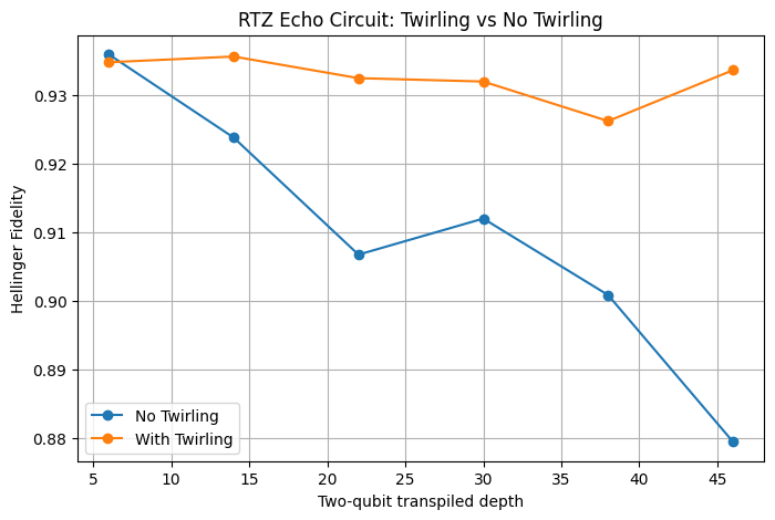
ตลอดบทเรียนนี้ เราได้พิจารณากรณีที่ Pauli twirling ถูกใช้เพื่อจำกัดการสะสมข้อผิดพลาด coherent ซึ่งเป็นบริบทที่อาจอธิบายได้ว่าเป็น error suppression อย่างไรก็ตาม Pauli twirling มักมีประโยชน์มากกว่าในฐานะเครื่องมือสำหรับปรับรูปแบบพฤติกรรมของข้อผิดพลาด โดยแปลงข้อผิดพลาด coherent ให้อยู่ในรูปที่คาดเดาได้มากขึ้นและสร้างแบบจำลองได้ง่ายขึ้น ประโยชน์ของสิ่งนี้จะชัดเจนขึ้นในบริบทของเทคนิคการลดข้อผิดพลาดอย่าง zero-noise extrapolation (ZNE) ซึ่งอาศัยการปรับขนาด noise ที่คาดเดาได้อย่างสมเหตุสมผล เรื่องนี้จะกล่าวถึงในบทเรียนถัดไป