Pooled sample-based quantum diagonalization ของ Hamiltonian นิวเคลียร์

ประมาณการการใช้งาน: 32 วินาทีบนโปรเซสเซอร์ Nighthawk r2 (หมายเหตุ: เป็นเพียงค่าประมาณ เวลารันจริงของคุณอาจแตกต่างออกไป)

สิ่งที่จะได้เรียนรู้

• เรียนรู้ว่า Hamiltonian แบบ shell-model ของนิวเคลียส ซึ่งจัดตารางไว้ในฐาน $J$-coupled ของ orbital กลายเป็น Hamiltonian ของ qubit ใน $m$-scheme ได้อย่างไร โดยหนึ่ง qubit แทนหนึ่งสถานะอนุภาคเดี่ยว

• สร้าง excitation ansatz แบบคงที่และไม่ใช่ variational ซึ่งมุมต่าง ๆ ได้มาจาก second-order perturbation theory จึงไม่มีลูปการหาค่าเหมาะสมแบบคลาสสิก

• เปรียบเทียบ qubit excitation กับ fermionic excitation และวัดว่าการเลือกใช้แบบใดส่งผลต่อ ความลึกของ two-qubit ของชุดวงจรอย่างไร

• รัน self-consistent configuration recovery ด้วย qiskit-addon-sqd เมื่อ ปริมาณที่อนุรักษ์คือจำนวนนิวคลีออน, $M_J$ และพาริตี แทนที่จะเป็นจำนวนอิเล็กตรอนและสปิน

• ใช้เวิร์กโฟลว์เดียวกันตั้งแต่ปัญหา 24 qubit ที่ตรวจสอบได้อย่างแน่นอน ไปจนถึงปัญหา 40 qubit ที่มีสถานะฐานเกือบสองล้านสถานะ ซึ่งเกินขีดความสามารถ exact-diagonalization ของบทเรียนนี้

สิ่งที่ต้องรู้ก่อน

ก่อนเริ่ม ให้ทบทวนหัวข้อต่อไปนี้

• Sample-based quantum diagonalization และ เอกสารอ้างอิง API ของ SQD addon

• Sample-based quantum diagonalization ของ Hamiltonian ทางเคมี ซึ่งเป็นคู่ฝั่งโครงสร้างอิเล็กตรอนของบทเรียนนี้

• Transpile ไปยัง backend target และ แนะนำ primitives

• Second quantization และการแมปแบบ Jordan-Wigner

ความเป็นมา

nuclear shell model มองนิวเคลียสเป็นนิวคลีออน valence จำนวนไม่กี่ตัวที่เคลื่อนที่ในชุด orbital อนุภาคเดี่ยวชุดเล็ก ๆ เหนือ core ที่เฉื่อย โดยมีอันตรกิริยาผ่านแรงสองวัตถุเชิงประจักษ์ ที่ปรับให้เข้ากับสเปกตรัมที่วัดได้ โมเดลนี้ใช้กันอย่างกว้างขวางในโครงสร้างนิวเคลียสพลังงานต่ำ ต้นทุนการคำนวณเป็นแบบ combinatorial คือฐานประกอบด้วยทุกวิธีที่จะกระจายโปรตอนและนิวตรอน valence ไปตาม สถานะที่มี และการเติบโตนี้จำกัดขนาดของ model space ที่ exact diagonalization เข้าถึงได้

Pooled sample-based quantum diagonalization (pooled SQD) [1] แบ่งปัญหานั้นออกเป็นสองส่วน วงจรควอนตัมถูกใช้เพียงเพื่อ เสนอ ว่าสถานะฐานใดสำคัญ โดยวัดในฐาน computational และแต่ละ bitstring ที่วัดได้ระบุ Slater determinant หนึ่งตัว จากนั้น Hamiltonian จะถูกสร้างและทำ diagonalization แบบคลาสสิกในปริภูมิที่ขยายโดย determinant เหล่านั้น เนื่องจากขั้นตอนคลาสสิก คือ exact diagonalization ภายในปริภูมิย่อย จึงให้ขอบบนแบบ variational ของพลังงานสถานะพื้นที่แท้จริง และขอบนี้มีแต่จะลดลงเมื่อเพิ่ม determinant

การแบ่งงานเช่นนี้ทำให้วิธีนี้ทนต่อสัญญาณรบกวนได้ แต่มีข้อจำกัดสำคัญ สัญญาณรบกวนเปลี่ยนว่าวงจร เสนอ determinant ตัวใด แต่ไม่เข้าไปอยู่ใน Hamiltonian แบบคลาสสิก จึงไม่สามารถเลื่อนค่าไอเกนของ ปริภูมิย่อยที่กำหนดได้ shot ที่ละเมิดปริมาณอนุรักษ์จะถูกทิ้งหรือซ่อมแซม และ shot ที่ รอดมาก็เป็นเวกเตอร์ฐานที่ถูกต้องไม่ว่าจะเกิดขึ้นด้วยวิธีใด ดังนั้นสัญญาณรบกวนทำให้คุณเสียคุณภาพ ของปริภูมิย่อย ไม่ใช่ความถูกต้อง และตัวเลขที่คุณรายงานเป็นขอบบนไม่ว่ากรณีใด

โครงสร้างนิวเคลียสให้เลขควอนตัมที่แน่นอนหลายตัวสำหรับกรองตัวอย่าง determinant ทางกายภาพต้องมีจำนวนโปรตอน valence ที่ถูกต้อง และ จำนวนนิวตรอน valence ที่ถูกต้อง มีโมเมนตัมเชิงมุมรวมภาพฉาย $M_J$ ที่ถูกต้อง และ พาริตีที่ถูกต้อง แต่ละอย่างตรวจสอบได้ด้วยการทดสอบจำนวนเต็มบน bitstring สัดส่วนของตัวอย่างที่ถูกปฏิเสธ ขึ้นอยู่กับข้อจำกัดและ model space

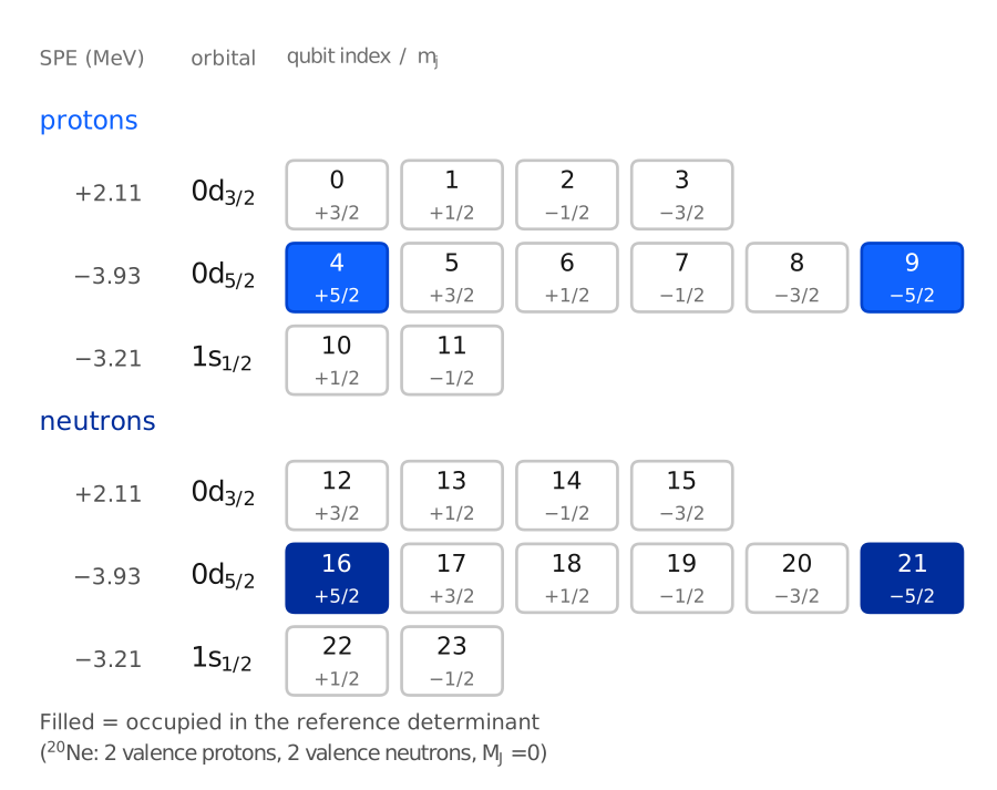
ทุก qubit คือสถานะอนุภาคเดี่ยวใน $m$-scheme หนึ่งสถานะ $(n, \ell, j, m_j, t_z)$ และ $|1\rangle$ หมายถึง ถูกครอบครอง รีจิสเตอร์ใช้ลำดับคงที่ คือโปรตอนก่อน แล้วจึงนิวตรอน ภายในแต่ละชนิด orbital เรียงตามลำดับในไฟล์ ภายในแต่ละ orbital เรียง $m_j$ จากมากไปน้อย ดังนั้นสองครึ่งของ bitstring จึงเป็นการจัดเรียงของโปรตอนและการจัดเรียงของนิวตรอน นี่คือการแบ่งสองส่วน ที่เครื่องมือหลังประมวลผลของ pooled SQD คาดหวัง

เวิร์กโฟลว์

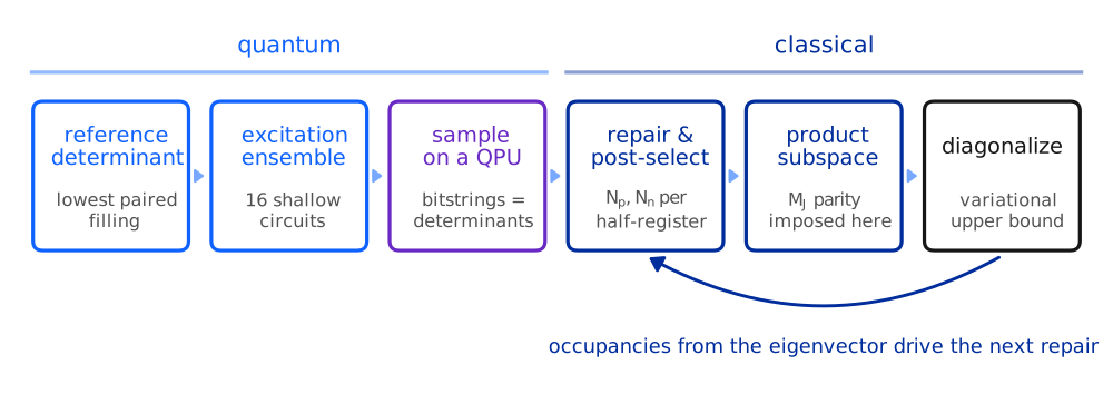
สองขั้นตอนในแผนภาพจัดการกับสมมาตรของนิวเคลียส

Repair และ post-selection จัดการกับตัวอย่างที่ได้รับผลจากสัญญาณรบกวนของฮาร์ดแวร์ จำนวนนิวคลีออนของสองครึ่งรีจิสเตอร์ คือ Hamming weight ดังนั้น qiskit-addon-sqd จึงจัดการได้โดยตรง recover_configurations ซ่อมแซม bitstring ที่เสียโดยพลิกบิตที่สอดคล้องน้อยที่สุดกับค่าประมาณปัจจุบันของการครอบครอง orbital เฉลี่ย แทนที่จะทิ้ง shot นั้นไป

ปริภูมิย่อยแบบผลคูณ นำ $M_J$ เข้ามา เนื่องจาก $M_J = M_p + M_n$ เชื่อมสองครึ่งเข้าด้วยกัน จึงไม่ใช่คุณสมบัติของครึ่งใดครึ่งหนึ่ง และต้องไม่ใช้กรองทั้ง shot bitstring ที่ครึ่งโปรตอนและครึ่งนิวตรอน ต่างก็ถูกต้องยังคงให้ half-configuration ที่ดีสองตัว แม้ $M_J$ รวมจะผิด ปริภูมิย่อยจึงถูกขยายโดย ผลคูณ ทุกคู่ของ การจัดเรียงโปรตอนที่สุ่มได้กับการจัดเรียงนิวตรอนที่สุ่มได้ โดยเก็บผลคูณที่อยู่ในเซกเตอร์ $M_J$ และพาริตีเป้าหมาย นี่คือการสร้างปริภูมิย่อยของ pooled SQD และหมายความว่า bitstring เพียงไม่กี่พัน ตัวสามารถขยายปริภูมิย่อยที่ใหญ่กว่าจำนวนตัวอย่างมาก

สมการหลักสองสมการ

Hamiltonian ของ shell-model คือพจน์หนึ่งวัตถุบวกอันตรกิริยาสองวัตถุ

$$\begin{equation} \tag{1} H = \sum_{p} \varepsilon_p\, a_p^\dagger a_p + \tfrac{1}{4}\sum_{pqrs} \langle pq \| rs \rangle\, a_p^\dagger a_q^\dagger a_s a_r , \end{equation}$$

โดย $p,q,r,s$ ระบุสถานะใน $m$-scheme และ $t_z = -1$ สำหรับโปรตอน $+1$ สำหรับนิวตรอน อันตรกิริยา เชิงประจักษ์ เช่น USDA [2] และ GXPF1 [3] ถูกจัดตารางไว้ไม่ใช่ใน $m$-scheme แต่ในฐาน $J$-coupled เป็นสมาชิกเมทริกซ์ $\langle ab; J | V | cd; J \rangle$ ระหว่างสถานะสองวัตถุแบบ antisymmetrized ที่ถูก normalize ของ orbital $a,b,c,d$ การกู้ สมาชิกใน $m$-scheme คือการ recoupling แบบ Clebsch-Gordan

$$\begin{equation} \tag{2} \langle pq \| rs \rangle = \sqrt{1 + \delta_{ab}}\sqrt{1 + \delta_{cd}} \sum_{J} \langle j_p m_p\, j_q m_q | J M \rangle \langle j_r m_r\, j_s m_s | J M \rangle \langle ab; J | V | cd; J \rangle , \end{equation}$$

โดยตัวประกอบ $\sqrt{1+\delta}$ ย้อนการ normalize ตามข้อตกลงของสถานะที่จัดตารางไว้ ทุกอย่างที่เหลือในบทเรียนนี้สร้างบนสองสมการนี้

การรันสามครั้ง

	นิวเคลียส	Shell	Qubits	ฐานที่สมมาตรอนุญาต	ตรวจสอบได้แน่นอนหรือไม่
ขนาดเล็ก	$^{20}\mathrm{Ne}$ (2p + 2n)	$sd$	24	640	ได้
ขนาดใหญ่	$^{44}\mathrm{Ti}$ (2p + 2n)	$pf$	40	4,000	ได้
ขนาดใหญ่	$^{48}\mathrm{Cr}$ (4p + 4n)	$pf$	40	1,963,461	ไม่ได้

การรันขนาดเล็กคือตัวอย่างการเดินผ่านทีละขั้น การรันขนาดใหญ่ทั้งสองใช้รีจิสเตอร์ 40 qubit ครั้งแรก ยังเล็กพอที่จะทำ diagonalization แบบแน่นอนบนแล็ปท็อปได้ คุณจึงเปรียบเทียบผลจากฮาร์ดแวร์กับค่าอ้างอิงที่แน่นอนได้ ครั้งที่สองเกิน ขีดความสามารถ exact-diagonalization ของบทเรียนนี้

ทุกการรันที่นี่ทำงานบน QPU นี่เป็นทางเลือกสำหรับบทเรียนนี้ ไม่ใช่ ข้อกำหนดของวิธีการ ทั้งสามการรันใช้ backend และงบประมาณ gate เดียวกัน เพื่อให้คุณเปรียบเทียบประสิทธิภาพ ที่ขนาดปัญหาต่างกันได้

ข้อกำหนด

ติดตั้งแพ็กเกจต่อไปนี้ก่อนเริ่ม

• Qiskit SDK v2.0 ขึ้นไป (pip install qiskit)

• qiskit-ibm-runtime v0.40 or later (pip install qiskit-ibm-runtime)

• SQD addon v0.12 ขึ้นไป (pip install qiskit-addon-sqd)

• NumPy, SciPy และ Matplotlib (pip install numpy scipy matplotlib)

คุณยังต้องมีบัญชี IBM Quantum® ที่บันทึกข้อมูลรับรองไว้ในเครื่อง และสิทธิ์เข้าถึง QPU ที่มีอย่างน้อย 40 qubit

ไม่ต้องใช้แพ็กเกจจำลอง และไม่ต้องดาวน์โหลดไฟล์ข้อมูลใด ๆ ไฟล์อันตรกิริยาสองไฟล์ ที่บทเรียนนี้ใช้ถูกฝังไว้ในเซลล์ตั้งค่าต่อไปนี้ และเขียนลงไดเรกทอรีชั่วคราวเมื่อคุณ รันเซลล์นั้น

การตั้งค่า

ส่วนนี้นำเข้าเครื่องมือและกำหนดตัวช่วยของ shell-model ที่เวิร์กโฟลว์ต้องใช้ ตามลำดับ ที่เวิร์กโฟลว์ใช้ ฟิสิกส์เบื้องหลังแต่ละตัวถูกอนุมานไว้ใน ภาคผนวก ส่วน คอมเมนต์อธิบายบทบาทของแต่ละฟังก์ชันในเวิร์กโฟลว์

ไฟล์อันตรกิริยาสองไฟล์ถูกแตกออกก่อน ทั้งสองเป็นชุดพารามิเตอร์ที่เผยแพร่แล้ว ฝังไว้ที่นี่เพื่อให้ โน้ตบุ๊กอยู่ได้ด้วยตัวเอง usda.snt คือ Hamiltonian ของ shell $sd$ แบบ USDA [2] และ gxpf1.snt คือ Hamiltonian ของ shell $pf$ แบบ GXPF1 [3]

# Added by doQumentation — installs the packages this notebook needs if they are missing
import importlib.util

_needed = {"matplotlib": "matplotlib", "numpy": "numpy", "qiskit": "qiskit", "qiskit_addon_sqd": "qiskit-addon-sqd", "qiskit_ibm_runtime": "qiskit-ibm-runtime", "scipy": "scipy"}
_missing = [pip for module, pip in _needed.items()
            if importlib.util.find_spec(module) is None]
# One at a time, so a package that fails to install does not block the others
for _pip in _missing:
    %pip install -q {_pip}
if not _missing:
    print("\u2713 All required packages are installed")

from __future__ import annotations

import base64
import gzip
import itertools
import tempfile
from dataclasses import dataclass
from functools import lru_cache
from math import factorial, sqrt
from pathlib import Path

import matplotlib.pyplot as plt
import numpy as np

from qiskit import QuantumCircuit
from qiskit.circuit.library import PauliEvolutionGate
from qiskit.quantum_info import Operator, SparsePauliOp
from qiskit.transpiler.preset_passmanagers import generate_preset_pass_manager
from qiskit_addon_sqd.configuration_recovery import recover_configurations
from qiskit_addon_sqd.counts import bit_array_to_arrays
from qiskit_addon_sqd.subsampling import postselect_by_hamming_right_and_left
from qiskit_ibm_runtime import QiskitRuntimeService, SamplerV2

from scipy.linalg import eigh

_USDA_SNT_GZ = (
    "H4sIAI5wqWoC/4WY224bRwyG7/UU9F0CONsZco5AUyBuC/QmQNG06KWhWGql1LYMy+kJefiOTrucGXJrQAgsf5nl8ecOr+CX"
    "D9+9g/0K9pv1/T389rx7gPLrsH+Cz/vVctg+vgAsrgB+HeDdAD9t7zYv6+dr+DDA+z8223/X17B8XMFN+ev9+m+4ed799XjA"
    "f9z8sy/4+s8BvoWYrsEERwbhFRqTXi+uCvOwW63vYf+0vFvDAgDo/AFIh8/hK7DH30354Omvb8o3V8c/vIUnMKtboK/wiGKF"
    "+gnFEfVn9PQUe8bthNIRtftbsGfUtQbAGXUFfawM8K0BF9SP6MWA0BpwQcMRvRhwBSX86+fl3ct2d4jq4+eHa3hYv2x2q7fX"
    "AJuPy+fb3cP69+Uh4luAT8djv95++eGV/fj6y6dvFudnmcX4lGOoBmttNOVncTL2FLs3NGT0l++ndJTv0cR8/t6NUanP8WMI"
    "6nPC6C8/5wp+vnn//QLOP9ank3k2wRszkDn/Zwv15xiv41l2SDmjhuEFM4PJ0QkYcgzM4A1Jp1GDkcvtaWMAR9tosAa9huHk"
    "AtoUBYwaF8hGarAxOywgxnoeN+Se2smF4H3QMPZQ653XMJpOi6GyrcLcZJtzLgoYcdsOyXKibV1Aom0fikJO0VLUMDeW3kAl"
    "qQLWpd66qGE02eZ9lXqSPD3UWyl5DeOeGnINJnmaUggCVrtgh2DJNm3fVy8WF3LSMFa9hYga5iYX0IQsYK2nmTpJkoq81Acy"
    "jLTTnPEaxqo3JGcbvZMeGnJVbw6mf2cUqcIsO80nFdOFq8JoSlY+Zb7FfNNZlnw2PqOE8SL3PtlSJhJGXGqsDRjbh4bmocWy"
    "oiIxSxjv09JYgaxlGLZxA9EFFOImuIBt3EB04TK3Z5S8wizrrFCJQ4Xpgl9hzDYbu0LCNm6HzkJHweUkYazITalyF7NjGAnh"
    "FZJFQniFZFHnqWgbdZ6qtoX50VZhvEJ81TJe7AUcQozH8yQMJ8ymUS07jLin6LXT3FRIhmwSTmtbJpEjr2AsvM7E1ra+ZaiM"
    "NoxewZinBlPQTmPJyikn7TQ2630SbWuz4CLlwzuGhCHPqbUmRZQwpkiBDn1vsoQ55oKjbEvNNVgbXls0WvA0NKnPpku91Fkx"
    "pahhXPDJtxVCQkBcMtJD27I8VJGAhWYYlVuZzc5e+jSIZWnLa57nOQ1iWZY+jSE3GP5/QIKi5E1Agqi9BbMZiUjEWNwChqKq"
    "KTZY11ku5ca2Pqc4YKk1o2DstBjJC1htW2nAgEZ4aDdPvQmmmLeY4tWFt9Y3VAdlpW+oDcpa3zpM1jdUB2XV9agOyqrrcWZQ"
    "sq7vMMffBseux5l5yjoLZ+Yp6yzU5mmt5DgzT5mSozZPoVIknJmnTJFQHZRV12OrlvpFQFbycoGKOWiYfl9QlXySGtSUvL9W"
    "VJi/YG4grC4CmuCX6CZrKUsY64UyJolCQoZJqWeKhDOCzxQJNcGXbZMEX7EtzF+gvCI1npxjmKaW5Q06ewVjOY0u2+Y0kt5D"
    "JhlETS2P+5CqyIMYkCI1NK50SO3TarSR2qfVaKOZPmXjg2beVJmS01zqp/CSmvoqvNSOD/kaS+qUoSGaTM2yz83fdjtMvsZy"
    "xOv7N44Fff/GT5q5tXWYfB3jWND3b9yumUvK5SQnvK6w/VuHyfu3DpP3bx0m7984FvT9W4fJ+zceWq/v3zpM3r9xLOj7tw6T"
    "928X053QgGz/1mHy/u3yZ8lTtn/jWND3b74NiDx2vRbeep56Lbz1oPRaeOv9G0dmxofXPK33bx0m798C1B9RuP4DPJ0WcLAa"
    "AAA="
)

_GXPF1_SNT_GZ = (
    "H4sIAI5wqWoC/4WcQY8dtw3H7/kU41sCeF8lUqKkQw9NgbaXoEHQQ26BkdiIEWdt2E6L9tNXb9+ORIn8PwdZILB/S3I4IsW/"
    "ZiYvjr//+P3f4nG8ef/x+PDm4dOvr9+9++rF8d3l+Mf7x99fvTz+dTn++fnTH7/1//z28pfL8e3H9/95fHm8evzl+lffvf3f"
    "H59e/fb26L9zHN//+t9Pl+OH1/++HH89JL88gkQO8esfvjm+phDomyvW//39/S+v3x2fPrz6+fVX/dfS889B4fpz/aN43P7p"
    "f3Bw/ynH8fD0Zy+uf/fn48MR3vxU/kRXlp7Z+PzDiqUnNn74iW8sb3azYvm0m29s2uxGxabTbryx2cZ7nGzu7KOKV2y8g5Un"
    "dsZbbLyDLafd53irjXew9bR7jffF8fbx8+uPr37+/Pb941dPv3P93ZH4W/If6kUohXCm+Jbmh3yR0jicybwl9CFeuFILy908"
    "HtIlcrlZyCNJ2q6MdGi7ZVy4tlvHJS52Y71FnHp8D+HCIYTlQuYFhdsv0yVxzZB6vsxwaZwJUumkIjWB1POdDhcqlR2KVo85"
    "SoDU8NgdNodiZevqMUqB1LCVWsO2ZMQlyYs+bXEFk4m5bMJJlVgSpGjaouhQvFKxUIbUjIvI85hWW4FNvubyDnMxMkFKRc8V"
    "Uml65OhQW1x9fe3XOAtsZPXJ36TIX18SaoQUnysnZsHUXPfcKqTyaSu36FHbWg0tN0jxWIXEAVLzbqcqkMpj3T8lwlBp9RhD"
    "qpAaHpnzni9nRXPh6lDbysmJBVLzDtU71KztnDxqW1+JhDaKnTtUa4DUzH00Hp0VXQMHSM3c16irlpf7GEcN1dogpfpEDpAa"
    "WRUOBKl0UqkIQ2qs+5IYU6OvthbFodIaF6/9i51VeF0TLZSN2lfh9T729utQOqtXKi/dl/21mihhW+M+BpIKqblypDWHSntc"
    "mSA1O3nMe+6dHp0DEaRmXCU0h9p7dOYCqVm1MehOnvy7nWphSKnuu+Q++X2Ca4uQGrYkxp3yMkFLL0ygavPovmR64dhFY5QM"
    "KVK1XRxqX4UydlHCXU44hY1ydndKuUBK11BzqH1NNOKNMvt27PMXVUWBemSqCVIjrr4nYFtzTSQJkJp3O7se09p9YygCKVL7"
    "UN4opx5DNnE5q5AlerZ2jyExpEYmggTtMYFrzC1Bak58jetGeSvHenSip9ROik0m5lqdsxzjrCYhTM1uImOHYZzVPvnWjXIm"
    "0RoaKyqhjjlqiEE3uWoYHqopbT/KY0pDD+Xtx9d8lvI0n6U8zWcpT/NpQqDms5Sn+TRVoOazlKf5LOVpPk1VqPl05AI1n6U8"
    "zaepAjWfpTzNp6kKNZ/OQoGaz1Ke5rOUp/k0VaHm03mvUPOd1+esL6X5LOVpPkt5ms9SnubTVIGaz1Ke5rOUp/ks5Wk+TVWo"
    "+SzlaT69mgVqPk0VqPks5Wk+S3maT1MVaj5dPwVqPkt5mk9TFWo+S3ma77x/8z56ms9SnuazlKf5LOVpPkt5ms9SnubTVIWa"
    "z1Ke5jupfRWumk9TBWo+S3maz1Ke5rOUp/k0VaHms5Sn+XTnLVDzWcrTfJqqUPNZytN85/1z7rbSfJbyNN/5t06fUJrPUp7m"
    "OykvE7T0wgqqdmo+Mb3Q03yCO6bSfII7ptJ8gruc0nxi+pen+eROL5yaT3CXU5pPx1Sh5hNcj0rzCajHVfMJqMdV88mdesyu"
    "xwo1n+B6VJpPcD0qzSe4HpXmE1yPSvMJrkelwERVR4Waz1Ke5hNTQ3THoxO90nzFZMLTfAVnVWm+grOqNF/BWVWaTxMVar6C"
    "r1FpvgK6yar56vbja76onormu8/5ViqOrNblZH6l0NPAlRq9sKaIbaFnhis15tUuH/E1oieLK1XOTIgsz3ROap9XpQ/SJWqK"
    "bCYcKm6K4tp9iUqqzbd1j4qO+g2tpTV6sll1qLipk6fnw32/isDWPSruPborwz7x9eakKbbry6Gi7RN9nrhuHr4tPXXsVLT9"
    "vvTdKlUQ18i9Q0Wn+2ZOlYpva0yiDhXthNz69p4S+7ZG7h0q2jma+/BIIfm2RnU4VLQ9R6hG4iWryVurhorOlNbzEJr4tubk"
    "bim6e25iqbFbJY4MKfREfaXGNXKK2aF2BSapD6Oy5162yd1S5Og0iq3k5tua1WEpsus+ZO4ZS76tqU4sRc7+mAtJyL6teR8t"
    "RVbDUO9yXM2a2O6jQ5GjdCi3HKpva04dluK7J1uWGtFLjhFS6J2HlZpKhzOm0JsRK5XnmjD7Izv5av0eBd7zVb5IsVU6ffTN"
    "oQXf1peoeveNjZWaNURFZ0L8fTsX1s9hwO4eeHkOA3Z3Zct6ZOccgPAM0O91hR4ZPEcWMAPkdBWQvsdZj72xZuTRs2U95qFY"
    "a8FZHVQpy/Mhd55YbGmPew2VGB2PRvOVsNlib0orYbO1U8fi0cbF6uQhw7jUycMybYs/dSiKwGxyLB5tXEmdM5WM4lKnGLFm"
    "FFeaPTruK8ehlEcbV55n2yIwrnlOXorAuPKsxyIwrjz7l3greptzSgve+tqo2lLbcu9MQ4oiPDMpjzaueR8rUUZxqaql/T46"
    "k5WiCM9fyuNpy5uZpM9WkvfaxpS1Ndd96JKV2LflUdrW1idaKOT0HNMnTCdnT/OZvcOZv5RHG5fqAJFhXLO2WykwrtlzJkV4"
    "llMebVxp7kOUMopr7h1dSmcUl9LuxesT2z6kPOq4ttkkk7sj1/1JWWWnHvfdfVKE50LlUV+jObPqs2hO+zViytpSJ+CFSyu+"
    "LY+yttRM3gf3HH1bHmVtzR5NXZQXcI0epW1tdyh2d86a2O52F9vR6V8FUgTm1dWjjWuepZUgMK45k2cKMC6PIjD7rh6j+gpi"
    "0Y904b675/n2h3u6QteTedkoc7qy2LIeaUxpkXNAHgeV53khozOYxZb1qDpTrvAa+TxBClECvEbPlvWY5o4cA7zGNDSfFIbX"
    "6NmyHmd1SEnwGgfVJ6YKr9GzZT3KebdDZIYe5bzGQLFAj54t7XHXfDkmJ6v789r17e7iTEMrxXhmUh5tXHNmainCuObMVBOO"
    "y6MYzEyrx9MW2VMf4cC9NWlbzpmVoqytucPkIO12SsZ4/lKUtTX7V6LGsfi2phadlLa1nX89naUHc437uYnQni/nlEzWN/S8"
    "s7TVo41LvUsW9+pwqFBl79HsPYkVr/sK9GjjYnVWSzBfqjoowXx5FN+ZC6dHG5d6WybjfM15ouYE8+VRDObC1aOOa3v+WEJq"
    "Tlzb2VCRELOtbYEU47NH5dHGpd5nagzj0s+HAozLoxjMq6tHnfutHmNjblz23G/1qChra3rMOT6f3jGefRVlbamZKfR1COKa"
    "PWdS1tZcXy3mnMm3pd4IGpS1Nd9Uai0Wir6t+fxxUtrWPvu27M1MG8XJ1KMz+yqK8Vmt8mjjmn1CKmcUF88zhVIzimtOtZNi"
    "fO6rPGpbW9XGLrg50G5rfwNhUueu7swmEtI55yQ0m/RpqI3JPd15ujVtWY9TSbcxpSU8dSShAj16tk4b3r6dmUlI2/L27Ulp"
    "W7vKLFK3uByK4nI2VP19SFEJ7EOrRxvXyESr413YhPchLsssV/0dRlEJ70PKo7a1n/vWa1rLbsu8mTooa0up8tpyEd+Wep42"
    "KG1rf6su5ebkvpqztLzl3qltRSVc28ojmTM+9F2TwNm3Qgp9/eSeKnaNXFtwqH3nk1KaJE05M6ZDOdNjv9NJIvm2Zr+3lFeP"
    "EvqGnH1bM/eWMtNQvFCRHnzUlJlzXMqZYFKqHHLxbdFUFIbiu+8XWmo+50vL6R06l1u/PBO/asN8B5zAmdXTDtP7r8h+jeWL"
    "lFOPocYumti39SWq3v0iTvxdtDw9hhmUq9N6PbaqvzJyqyNeMi0nIm51LLbojgIrOUKP+l2yBj16tghrqxib1gqg0pLknfIq"
    "bdoirJqkMMNrnDNATPgaPVuE9VBv0J7HbU107V42W44eUhSjPrF4JKyHUokZxqXeTV+exAI9pCjGp/zKIwE9dO2+XSTX1vbc"
    "b6pJUYT1UOCWWw2+rdmZJkVYD1Ef0Uoi39acySdFWA9RztLVjm9LPQ0cFAENc3unJjrVsWuY0mK297EYxbrbcs7vlUfCGib3"
    "bQ/GNWffMijCGkZRDHr0w+KRsIbpnem6dnZbe9VOitTsW7e3I+e7Pgnv7tfHQxvl7O7KlvU4zu95fouUUNV21RSGFk2oHhdb"
    "ZGbf+b4cXf8nRlnb8maASVlbc+UkSnSb0hKox4eFIjNHz7c/aHydkvC6T9Lydo3Je+u8ZSdf+xsu06O2ta2vPr70W1l2W9v6"
    "UhSbPoG+kwYnSDVnTKGvqYvfv3JuDVLom2vvpOZpvh9fizHuX71jVp79vqDcG8rrJolLnecTxe8TgMLfBTDoJteOGUVntYJr"
    "5PHOVsKnUaEuJw8oE9MWA5V5e2tA9wmQrw5xQB6RrernS33VkEB1PCmKW5f7P6zudeW7TwAA"
)

DATA = Path(tempfile.mkdtemp(prefix="nuclear_sqd_"))
for name, blob in (("usda.snt", _USDA_SNT_GZ), ("gxpf1.snt", _GXPF1_SNT_GZ)):
    (DATA / name).write_bytes(gzip.decompress(base64.b64decode(blob)))

    if not (DATA / name).is_file():
        raise RuntimeError(f"{name} did not unpack to {DATA}")

model space และรีจิสเตอร์ qubit

ไฟล์ .snt เก็บ model space พลังงานอนุภาคเดี่ยว และสมาชิกเมทริกซ์สองวัตถุแบบ $J$-coupled สำหรับอันตรกิริยาที่ขึ้นกับมวลที่ใช้ที่นี่ ฟิลด์ที่สามและสี่ของส่วนหัวสองวัตถุ ระบุมวลอ้างอิง $A_{\mathrm{ref}}$ ที่ใช้ปรับอันตรกิริยา และเลขชี้กำลังของการขึ้นกับมวล ทั้งสอง ไฟล์มีเลขชี้กำลัง $-0.3$ โดย $A_{\mathrm{ref}} = 18$ สำหรับ USDA และ $42$ สำหรับ GXPF1 ดังนั้น สมาชิกเมทริกซ์ที่จัดตารางไว้ต้องถูกปรับสเกลด้วย $(A/A_{\mathrm{ref}})^{-0.3}$ ตามนิวเคลียสที่ กำลังคำนวณ [2], [3] พลังงานอนุภาคเดี่ยวไม่ถูกปรับสเกล หากข้าม ขั้นตอนนี้ พลังงานสหสัมพันธ์จะเปลี่ยนไปราวไม่กี่เปอร์เซ็นต์

พลังงานต่อจากนี้คือพลังงาน valence ซึ่งวัดจาก core ที่เฉื่อย ไม่ใช่พลังงานแยก ที่ได้จากการทดลอง

@dataclass(frozen=True)
class Orbital:
    idx: int
    n: int
    ell: int
    j2: int
    tz: int  # j2 = 2j; tz = -1 proton, +1 neutron

@dataclass(frozen=True)
class SPState:
    """One m-scheme single-particle state, i.e. one qubit."""

    orb: int
    j2: int
    mj2: int
    tz: int
    ell: int
    spe: float  # mj2 = 2 * m_j

@dataclass
class ModelSpace:
    orbitals: list
    spes: dict
    tbmes: dict
    core_z: int
    core_n: int
    mass_number: int
    a_ref: int
    mass_exponent: float
    mass_factor: float

def read_snt(path, n_protons, n_neutrons):
    """Parse a .snt interaction file, applying its mass dependence for this nucleus.

    The two-body header line is ``n_tbme  method  A_ref  exponent``.  When ``method`` is 1 the
    tabulated matrix elements are rescaled by ``(A / A_ref) ** exponent``, where A is the mass
    number of the whole nucleus -- the core plus the valence nucleons.  A is derived from the
    file's own core numbers rather than passed in, so it cannot silently disagree with the
    valence counts the rest of the workflow uses.  Single-particle energies are not rescaled.
    """
    rows = [
        ln.split("!")[0].split() for ln in Path(path).read_text().splitlines()
    ]
    rows = iter([r for r in rows if r])

    n_p_orb, n_n_orb, core_z, core_n = (int(x) for x in next(rows)[:4])
    orbitals = [
        Orbital(*(int(x) for x in next(rows)[:5]))
        for _ in range(n_p_orb + n_n_orb)
    ]

    spes = {}
    for _ in range(int(next(rows)[0])):  # "i  i  <i|H(1b)|i>"
        field = next(rows)
        spes[int(field[0])] = float(field[2])

    n_tbme, method, a_ref, exponent = next(rows)[:4]
    n_tbme, method, a_ref, exponent = (
        int(n_tbme),
        int(method),
        int(a_ref),
        float(exponent),
    )
    mass_number = core_z + core_n + n_protons + n_neutrons
    factor = (mass_number / a_ref) ** exponent if method == 1 else 1.0

    tbmes = {}
    for _ in range(n_tbme):  # "a  b  c  d  J  value"
        field = next(rows)
        tbmes[tuple(int(x) for x in field[:5])] = float(field[5]) * factor

    return ModelSpace(
        orbitals,
        spes,
        tbmes,
        core_z,
        core_n,
        mass_number,
        a_ref,
        exponent,
        factor,
    )

def m_scheme_states(ms):
    """The qubit register: protons then neutrons, orbitals in file order, m_j descending."""
    return [
        SPState(o.idx, o.j2, m2, o.tz, o.ell, ms.spes[o.idx])
        for tz in (-1, +1)
        for o in ms.orbitals
        if o.tz == tz
        for m2 in range(o.j2, -o.j2 - 1, -2)
    ]

การ recoupling แบบ Clebsch-Gordan

สมการ (2) ต้องใช้สัมประสิทธิ์ Clebsch-Gordan สำหรับโมเมนตัมเชิงมุมแบบครึ่งจำนวนเต็ม ทุกอาร์กิวเมนต์ ถูกส่งเป็น สองเท่า ของค่าทางกายภาพ ดังนั้น $j = 5/2$ จึงเข้ามาเป็น 5 และการคำนวณยังคงแน่นอน

Interaction.v_ms จัดการการค้นหาสมาชิกเมทริกซ์ของอันตรกิริยา ไฟล์ .snt เก็บแต่ละ สมาชิกเมทริกซ์เพียงครั้งเดียว การค้นหาจึงอาจต้องใช้เฟส pair-exchange แบบ antisymmetrized $-(-1)^{j_a + j_b - J}$ ที่ด้านใด ด้านหนึ่ง และ bra กับ ket อาจถูกเก็บในลำดับใดก็ได้

@lru_cache(maxsize=None)
def clebsch_gordan(j1_2, j2_2, J_2, m1_2, m2_2, M_2):
    """<j1 m1 j2 m2 | J M>.  Every argument is twice its physical value."""
    if m1_2 + m2_2 != M_2 or not abs(j1_2 - j2_2) <= J_2 <= j1_2 + j2_2:
        return 0.0
    if abs(m1_2) > j1_2 or abs(m2_2) > j2_2 or abs(M_2) > J_2:
        return 0.0
    if (j1_2 + j2_2 - J_2) % 2 or (j1_2 - m1_2) % 2 or (j2_2 - m2_2) % 2:
        return 0.0

    f, half = factorial, lambda x: x // 2
    prefactor = sqrt(
        (J_2 + 1)
        * f(half(j1_2 + j2_2 - J_2))
        * f(half(j1_2 - j2_2 + J_2))
        * f(half(-j1_2 + j2_2 + J_2))
        / f(half(j1_2 + j2_2 + J_2) + 1)
        * f(half(J_2 + M_2))
        * f(half(J_2 - M_2))
        * f(half(j1_2 - m1_2))
        * f(half(j1_2 + m1_2))
        * f(half(j2_2 - m2_2))
        * f(half(j2_2 + m2_2))
    )
    total = 0.0
    for k in range(half(j1_2 + j2_2 - J_2) + 1):
        d = [
            half(j1_2 + j2_2 - J_2) - k,
            half(j1_2 - m1_2) - k,
            half(j2_2 + m2_2) - k,
            half(J_2 - j2_2 + m1_2) + k,
            half(J_2 - j1_2 - m2_2) + k,
        ]
        if all(x >= 0 for x in d):
            total += (-1) ** k / (
                f(k) * f(d[0]) * f(d[1]) * f(d[2]) * f(d[3]) * f(d[4])
            )
    return prefactor * total

class Interaction:
    """Antisymmetrized m-scheme two-body matrix elements <pq||rs>, per Eq. (2)."""

    def __init__(self, model_space, sp):
        self.ms, self.sp, self._cache = model_space, sp, {}

    def _tbme(self, oa, ob, oc, od, J, j_ab_2, j_cd_2):
        """<oa ob; J|V|oc od; J>, allowing for how the file happens to order each pair."""
        table = self.ms.tbmes
        # |ba; J> = -(-1)^(j_a + j_b - J) |ab; J> for a normalized antisymmetrized pair;
        # dropping the leading minus makes v_ms symmetric instead of antisymmetric, and
        # the Hamiltonian then fails the rotational-invariance check in Step 1.
        phase_ab = -1.0 if (j_ab_2 // 2 - J) % 2 == 0 else 1.0
        phase_cd = -1.0 if (j_cd_2 // 2 - J) % 2 == 0 else 1.0
        for keys, phase in (
            (((oa, ob, oc, od), (oc, od, oa, ob)), 1.0),
            (((ob, oa, oc, od), (oc, od, ob, oa)), phase_ab),
            (((oa, ob, od, oc), (od, oc, oa, ob)), phase_cd),
            (((ob, oa, od, oc), (od, oc, ob, oa)), phase_ab * phase_cd),
        ):
            for key in keys:
                value = table.get(key + (J,))
                if value is not None:
                    return value * phase
        return 0.0

    def v_ms(self, p, q, r, s):
        """<pq||rs>, zero unless M_J and charge are conserved."""
        cached = self._cache.get((p, q, r, s))
        if cached is not None:
            return cached

        P, Q, R, S = (self.sp[i] for i in (p, q, r, s))
        value = 0.0
        if P.mj2 + Q.mj2 == R.mj2 + S.mj2 and P.tz + Q.tz == R.tz + S.tz:
            M = P.mj2 + Q.mj2
            # sqrt(1 + delta): undo the normalization of the tabulated pair states
            c12 = sqrt(2.0) if (P.tz == Q.tz and P.orb == Q.orb) else 1.0
            c34 = sqrt(2.0) if (R.tz == S.tz and R.orb == S.orb) else 1.0
            for J2 in range(
                max(abs(P.j2 - Q.j2), abs(R.j2 - S.j2)),
                min(P.j2 + Q.j2, R.j2 + S.j2) + 1,
                2,
            ):
                cg_bra = clebsch_gordan(P.j2, Q.j2, J2, P.mj2, Q.mj2, M)
                cg_ket = clebsch_gordan(R.j2, S.j2, J2, R.mj2, S.mj2, M)
                if abs(cg_bra) < 1e-12 or abs(cg_ket) < 1e-12:
                    continue
                value += (
                    c12
                    * c34
                    * cg_bra
                    * cg_ket
                    * self._tbme(
                        P.orb,
                        Q.orb,
                        R.orb,
                        S.orb,
                        J2 // 2,
                        P.j2 + Q.j2,
                        R.j2 + S.j2,
                    )
                )

        self._cache[(p, q, r, s)] = value
        return value

สมาชิกเมทริกซ์และการทดสอบสมมาตร

determinant คือ tuple ที่เรียงลำดับของดัชนี qubit ที่ถูกครอบครอง determinant สองตัวที่ต่างกันมากกว่า สองสถานะที่ถูกครอบครองจะมีสมาชิกเมทริกซ์เป็นศูนย์ มิฉะนั้นกฎ Slater-Condon ให้ผลรวม สั้น ๆ ของอันตรกิริยา คูณด้วยเครื่องหมายแบบเฟอร์มิออนที่นับจำนวนสถานะที่ถูกครอบครองระหว่าง ตัวดำเนินการในลำดับรีจิสเตอร์คงที่

symmetry_allowed คือการทดสอบจำนวนเต็มที่เลขควอนตัมแน่นอนทั้งสี่ลดรูปมาเป็น ใช้ทั้งเพื่อ กรองตัวอย่าง และเพื่อไล่ฐานที่แน่นอนสำหรับการรันที่เล็กพอจะตรวจสอบได้

def matrix_element(inter, det_a, det_b):
    """<A|H|B> for two determinants, each a sorted tuple of occupied qubit indices."""
    set_a, set_b = set(det_a), set(det_b)
    out_a, out_b = sorted(set_a - set_b), sorted(set_b - set_a)
    if len(out_a) != len(out_b) or len(out_a) > 2:
        return 0.0

    if not out_a:  # diagonal: one-body plus two-body
        return sum(inter.sp[i].spe for i in det_a) + sum(
            inter.v_ms(i, j, i, j)
            for i, j in itertools.combinations(det_a, 2)
        )

    if len(out_a) == 1:  # one state moves, p -> q
        p, q = out_a[0], out_b[0]
        crossings = sum(1 for k in set_a if min(p, q) < k < max(p, q))
        return (-1.0) ** crossings * sum(
            inter.v_ms(p, j, q, j) for j in det_a if j not in (p, q)
        )

    (p, r), (q, s) = out_a, out_b  # two states move
    crossings = sum(1 for k in set_a if p < k < r) + sum(
        1 for k in set_b if q < k < s
    )
    return (-1.0) ** crossings * inter.v_ms(p, r, q, s)

def subspace_hamiltonian(inter, dets):
    """Dense real-symmetric H projected onto the span of `dets`."""
    H = np.zeros((len(dets), len(dets)))
    for a, det_a in enumerate(dets):
        H[a, a] = matrix_element(inter, det_a, det_a)
        for b in range(a + 1, len(dets)):
            H[a, b] = H[b, a] = matrix_element(inter, det_a, dets[b])
    return H

def ground_state(inter, dets):
    """Lowest eigenvalue and eigenvector of H over `dets`."""
    values, vectors = np.linalg.eigh(subspace_hamiltonian(inter, dets))
    return values[0], vectors[:, 0]

def symmetry_allowed(
    sp, det, n_protons, n_neutrons, mj2_target=0, parity_target=0
):
    """The four exact shell-model quantum numbers, as integer tests on one determinant."""
    n_p = sum(1 for i in det if sp[i].tz == -1)
    return (
        n_p == n_protons
        and len(det) - n_p == n_neutrons
        and sum(sp[i].mj2 for i in det) == mj2_target
        and sum(sp[i].ell for i in det) % 2 == parity_target
    )

def full_basis(sp, n_protons, n_neutrons, **targets):
    """Every symmetry-allowed determinant.  Only tractable for small model spaces."""
    protons = [i for i, s in enumerate(sp) if s.tz == -1]
    neutrons = [i for i, s in enumerate(sp) if s.tz == +1]
    return [
        p + n
        for p in itertools.combinations(protons, n_protons)
        for n in itertools.combinations(neutrons, n_neutrons)
        if symmetry_allowed(sp, p + n, n_protons, n_neutrons, **targets)
    ]

def count_basis(sp, n_protons, n_neutrons, mj2_target=0, parity_target=0):
    """How many determinants `full_basis` would return, without enumerating them.

    A dynamic program over (occupied count, sum of 2*m_j, parity) per species.  This stays
    cheap when the basis itself is far too large to build, which is how the largest run below
    can report the size of the space it is sampling from.
    """

    def species(states, k):
        table = {(0, 0, 0): 1}
        for s in states:
            for key, value in list(table.items()):
                count, m_sum, parity = key
                if count < k:
                    nxt = (count + 1, m_sum + s.mj2, (parity + s.ell) % 2)
                    table[nxt] = table.get(nxt, 0) + value
        totals = {}
        for (count, m_sum, parity), value in table.items():
            if count == k:
                totals[(m_sum, parity)] = (
                    totals.get((m_sum, parity), 0) + value
                )
        return totals

    left = species([s for s in sp if s.tz == -1], n_protons)
    right = species([s for s in sp if s.tz == +1], n_neutrons)
    return sum(
        a * b
        for (mp, pp), a in left.items()
        for (mn, pn), b in right.items()
        if mp + mn == mj2_target and (pp + pn) % 2 == parity_target
    )

determinant อ้างอิง

ansatz ถูกสร้างบน determinant ตัวเดียว ดังนั้น determinant นั้นควรเป็นตัวที่ดีที่สุด เท่าที่มี การเติมพลังงานอนุภาคเดี่ยวต่ำสุดละเลยอันตรกิริยาสองวัตถุ ใน model space เหล่านี้ ตัวเลือกนั้นให้พลังงานสูงกว่า determinant พลังงานต่ำสุด 1–2 MeV

การจำกัดเฉพาะการเติมที่ประกอบด้วยคู่ time-reversed $(+m_j, -m_j)$ บังคับให้ $M_J = 0$ อย่างแน่นอน และ เหลือผู้สมัครเพียง $\binom{n_{\mathrm{pairs}}}{k}$ ตัวต่อชนิด (อย่างมากไม่กี่พัน) จึง หาตัวที่ดีที่สุดได้โดยค้นทั้งหมดบนเส้นทแยงเต็ม $\langle \Phi | H | \Phi \rangle$ กรณีเสมอให้ตกแก่คู่ที่เรียงตัวแรงที่สุด ซึ่งแรง pairing แบบ $J = 0$ แรงที่สุด ในทุก กรณีในบทเรียนนี้ที่ตรวจสอบกับการไล่แจงเต็มได้ การค้นหาคืนค่า determinant ที่มีเส้นทแยงต่ำสุดระดับโลก ซึ่งเป็นองค์ประกอบเดี่ยวที่ใหญ่ที่สุดของสถานะพื้นที่แน่นอนด้วย

def reference_determinant(sp, inter, n_protons, n_neutrons):
    """Lowest-diagonal determinant built from time-reversed (+m_j, -m_j) orbital pairs."""
    if n_protons % 2 or n_neutrons % 2:
        raise ValueError(
            "an odd valence count has no time-reversed paired reference at M_J = 0"
        )

    def species_pairs(tz):
        return [
            (
                q,
                next(
                    p
                    for p, t in enumerate(sp)
                    if t.tz == tz and t.orb == s.orb and t.mj2 == -s.mj2
                ),
            )
            for q, s in enumerate(sp)
            if s.tz == tz and s.mj2 > 0
        ]

    best = None
    for chosen_p in itertools.combinations(species_pairs(-1), n_protons // 2):
        protons = tuple(q for pair in chosen_p for q in pair)
        for chosen_n in itertools.combinations(
            species_pairs(+1), n_neutrons // 2
        ):
            det = tuple(
                sorted(protons + tuple(q for pair in chosen_n for q in pair))
            )
            # break ties toward the most aligned pairs, where J = 0 pairing is strongest
            score = (
                matrix_element(inter, det, det),
                -sum(abs(sp[q].mj2) for q in det),
            )
            if best is None or score < best[0]:
                best = (score, det)
    return best[1]

พูลของ excitation และการจัดอันดับเชิง perturbative

สหสัมพันธ์ถูกพาโดย excitation แบบ two-particle–two-hole ($2p2h$) จากตัวอ้างอิง กฎการเลือกสองข้อ ลดพูลก่อนสร้างวงจรใด ๆ excitation ต้องอนุรักษ์ $M_J$ และคู่ hole กับคู่ particle ต้องสามารถ couple ไปยัง $J$ รวมร่วมกันได้ ซึ่งคืออสมการสามเหลี่ยม

excitation ที่เหลือถูกจัดอันดับด้วยคะแนนอันดับสองของ Epstein-Nesbet ของ selected configuration interaction [4]

$$\begin{equation} \tag{3} s_\alpha = \frac{|\langle \Phi_{\mathrm{ref}} | H | \alpha \rangle|^2}{|\Delta_\alpha|}, \qquad \Delta_\alpha = H_{\mathrm{ref},\mathrm{ref}} - H_{\alpha\alpha}, \end{equation}$$

ซึ่งประมาณว่า excitation แต่ละตัวพาพลังงานสหสัมพันธ์เท่าใด สองจำนวนเดียวกันนี้กำหนด มุมของวงจร เมื่อ $V = \langle \Phi_{\mathrm{ref}} | H | \alpha \rangle$ แอมพลิจูดอันดับหนึ่ง คือ $t_\alpha = V / \Delta_\alpha$ ภาคผนวก อธิบายว่าทำไมแอมพลิจูดอันดับหนึ่งจึงเป็น ตัวเลือกที่ใช้ในบทเรียนนี้ แทนที่จะเป็นมุมสองระดับที่แน่นอน

def excitation_pool(sp, occ):
    """2p2h quadruples (h1, h2, v1, v2): same-species pairs, then proton-neutron pairs."""
    holes = {tz: [i for i in occ if sp[i].tz == tz] for tz in (-1, +1)}
    virtuals = {
        tz: [i for i, s in enumerate(sp) if s.tz == tz and i not in occ]
        for tz in (-1, +1)
    }
    pool = [
        (h1, h2, v1, v2)
        for tz in (-1, +1)
        for h1, h2 in itertools.combinations(holes[tz], 2)
        for v1, v2 in itertools.combinations(virtuals[tz], 2)
    ]
    pool += [
        (h1, h2, v1, v2)
        for h1 in holes[-1]
        for h2 in holes[+1]
        for v1 in virtuals[-1]
        for v2 in virtuals[+1]
    ]
    return pool

def conserves_symmetry(sp, op):
    """Keeps M_J, and the hole and particle pairs share a reachable total J."""
    h1, h2, v1, v2 = op
    if sp[v1].mj2 + sp[v2].mj2 != sp[h1].mj2 + sp[h2].mj2:
        return False
    return max(abs(sp[v1].j2 - sp[v2].j2), abs(sp[h1].j2 - sp[h2].j2)) <= min(
        sp[v1].j2 + sp[v2].j2, sp[h1].j2 + sp[h2].j2
    )

def en_denominator(inter, occ, holes, virtuals, floor=0.1):
    """Epstein-Nesbet gap: bare gap, spectator rearrangement, and the pair's own term."""
    gap = sum(inter.sp[h].spe for h in holes) - sum(
        inter.sp[v].spe for v in virtuals
    )
    for k in occ:
        if k in holes:
            continue
        gap += sum(inter.v_ms(h, k, h, k) for h in holes)
        gap -= sum(inter.v_ms(v, k, v, k) for v in virtuals)
    gap += inter.v_ms(holes[0], holes[1], holes[0], holes[1])
    gap -= inter.v_ms(virtuals[0], virtuals[1], virtuals[0], virtuals[1])
    return gap if abs(gap) >= floor else (floor if gap >= 0 else -floor)

def rank_pool(inter, occ, pool):
    """Sort by descending PT2 score; return (operator, coupling, first-order amplitude)."""
    ranked = []
    for op in pool:
        h1, h2, v1, v2 = op
        coupling = inter.v_ms(v1, v2, h1, h2)
        gap = en_denominator(inter, occ, (h1, h2), (v1, v2))
        ranked.append((coupling**2 / abs(gap), op, coupling, coupling / gap))
    ranked.sort(key=lambda row: (-row[0], row[1]))  # deterministic on ties
    return [
        (op, coupling, amplitude) for _, op, coupling, amplitude in ranked
    ]

บล็อก qubit-excitation

ภายใต้การแมปแบบ Jordan-Wigner ตัวดำเนินการ excitation $2p2h$ ที่อนุรักษ์จำนวนอนุภาคกลายเป็นผลรวมของ Pauli string แปดตัว แต่ละตัวมี string ของตัวดำเนินการ $Z$ ระหว่างดัชนีนอกสุด string $Z$ บังคับใช้ antisymmetry ของเฟอร์มิออน และมีราคาแพง excitation แบบโปรตอน-นิวตรอน คร่อมขอบเขตระหว่างสองครึ่งของรีจิสเตอร์ และรวม parity string ข้ามขอบเขตนั้น

การตัด string $Z$ ออกให้ตัวดำเนินการ qubit-excitation ของ Yordanov et al. [5] สถานะที่เตรียมโดยตัวดำเนินการนี้มีแอมพลิจูดต่างออกไป แต่เชื่อมคู่ determinant ชุดเดียวกันทุกประการ ดังนั้นเซตของ determinant ที่วงจร เข้าถึงได้จึงไม่เปลี่ยน Pooled SQD ใช้ determinant เหล่านี้สำหรับ diagonalization แบบคลาสสิก Step 2 เปรียบเทียบ support ของสองการสร้างและวัดต้นทุนบนฮาร์ดแวร์ของทั้งสอง

การสร้างรูป Pauli จาก $a_j^\dagger = \tfrac{1}{2}(X_j - i Y_j) \otimes Z_{<j}$ โดยให้ string $Z$ เลือกได้ ทำให้สองการสร้างต่างกันเพียงแฟลกเดียว พจน์ทั้งแปดของหนึ่งตัวกำเนิด สลับที่กันได้ ดังนั้นขั้น PauliEvolutionGate เพียงขั้นเดียวจึงเป็นเอกซ์โปเนนเชียลที่แน่นอน ไม่ใช่การประมาณแบบ Trotter ของมัน

def _ladder(num_qubits, q, dagger, parity):
    """Pauli form of a_q or a_q^dagger.  `parity` toggles the Jordan-Wigner Z string."""
    prefix = (
        ["Z"] * q + ["I"] * (num_qubits - q) if parity else ["I"] * num_qubits
    )
    x_part, y_part = list(prefix), list(prefix)
    x_part[q], y_part[q] = "X", "Y"
    return SparsePauliOp(
        ["".join(reversed(x_part)), "".join(reversed(y_part))],
        coeffs=[0.5, 0.5 * (-1j if dagger else 1j)],
    )

def excitation_generator(num_qubits, op, parity=False):
    """Hermitian H with exp(-i theta H) = exp(theta (T - T^dagger)) for T = a+ a+ a a."""
    h1, h2, v1, v2 = op
    T = SparsePauliOp("I" * num_qubits)
    for q, dagger in ((v1, True), (v2, True), (h2, False), (h1, False)):
        T = (T @ _ladder(num_qubits, q, dagger, parity)).simplify()
    return (1j * (T - T.adjoint())).simplify()

def excitation_block(op, theta, parity=False):
    """(window, circuit) for one excitation.

    A qubit excitation touches only its four qubits.  A fermionic excitation also carries Z
    operators on every qubit between the outermost indices, so its window is the whole span --
    which is exactly where its extra cost comes from.
    """
    window = list(range(min(op), max(op) + 1)) if parity else sorted(op)
    local = tuple(window.index(i) for i in op)
    generator = excitation_generator(len(window), local, parity=parity)
    return window, PauliEvolutionGate(generator, time=theta).definition

def excitation_ansatz(
    num_qubits, occ, operators, amplitudes, measure=True, parity=False
):
    """X gates for the reference determinant, then one evolution block per excitation."""
    qc = QuantumCircuit(num_qubits)
    for q in occ:
        qc.x(q)
    for op, theta in zip(operators, amplitudes):
        if abs(theta) < 1e-12:
            continue
        window, block = excitation_block(op, theta, parity=parity)
        qc.compose(block, qubits=window, inplace=True)
    if measure:
        qc.measure_all()
    return qc

งบประมาณความลึกและชุดวงจร

วงจรลึกวงจรเดียวที่มีทุก excitation ที่จัดอันดับอาจเกินเวลาโคฮีเรนซ์ของฮาร์ดแวร์ การกระจายพูล ไปยัง ชุด ของวงจรตื้น ๆ และรวม shot ของพวกมันเป็นเซต determinant เดียว ทำให้ Step 2 กลายเป็นปัญหาการบรรจุ คือแต่ละ excitation มีต้นทุนที่วัดได้ แต่ละวงจรมีงบประมาณ และ คำถามคือพูลที่จัดอันดับไว้ใส่ได้มากเท่าใด

งบประมาณวัดเป็น two-qubit depth (จำนวนชั้นของ gate สอง qubit บนเส้นทางวิกฤต) แทนจำนวน gate ดิบ เพราะความลึกกำหนดระยะเวลาของวงจร และจึงกำหนดว่า ใช้โคฮีเรนซ์ของอุปกรณ์ไปมากเท่าใด จำนวนรวมถูกรายงานควบคู่กัน เพราะเป็น ตัวแทนที่ดีกว่าของความคลาดเคลื่อนของ gate สะสม ทั้งสองตอบคำถามต่างกันและไม่มีอันใดทดแทน อีกอันได้

ทั้งสองปริมาณถูกดึงตาม arity คือคำสั่งที่ทำงานกับสอง qubit พอดี ไม่ว่า backend จะเรียก entangling gate ของมันว่าอะไร การจับคู่ตามชื่อ gate แทนอาจให้ค่าเป็นศูนย์ สำหรับชุด basis ที่ไม่คุ้นเคย ทำให้ใส่ทั้งพูลในวงจรเดียวโดยไม่ถูกต้อง โดยไม่เกิน งบประมาณที่คำนวณได้

การเติมวงจรที่ว่างที่สุดในขณะนั้นตามลำดับอันดับ ทำให้ทุกวงจรใกล้งบประมาณ ต้นทุนถูกวัดบน target ของ backend จริง ทีละ excitation เพราะต้นทุนที่อ่านจาก วงจรนามธรรมไม่ใช่ต้นทุนที่ transpiler สร้างขึ้นจริง

DIRECTIVES = ("barrier", "delay")

def is_two_qubit(instruction):
    """True for an operation on exactly two qubits, excluding directives.

    Selecting by arity rather than by gate name keeps this correct on any backend, whatever its
    two-qubit basis gate happens to be called -- cz on today's Heron devices, ecr on Eagle, or
    something newer tomorrow.  A gate-name allow-list silently returns zero on anything it has
    not heard of, which would collapse the whole pool into one circuit and pass every budget
    check.  Barriers are excluded because a barrier spanning two qubits is not a gate.
    """
    return (
        len(instruction.qubits) == 2
        and instruction.operation.name not in DIRECTIVES
    )

def two_qubit_count(qc):
    """How many two-qubit gates the circuit contains: the accumulated-gate-error proxy."""
    return sum(1 for instruction in qc.data if is_two_qubit(instruction))

def two_qubit_depth(qc):
    """Layers of two-qubit gates on the critical path: the duration and decoherence proxy.

    This is what the budget is measured in.  Two gates on disjoint qubit pairs run in the same
    layer, so depth tracks how long the circuit takes -- and therefore how much coherence it
    spends -- while the count above tracks how much gate error it accumulates.  Both are
    reported; only depth is budgeted.
    """
    return qc.depth(filter_function=is_two_qubit)

def excitation_costs(num_qubits, ranked, pm, parity=False):
    """Transpiled two-qubit depth of each excitation on its own."""
    return [
        two_qubit_depth(
            pm.run(
                excitation_ansatz(
                    num_qubits, (), [op], [amp], measure=False, parity=parity
                )
            )
        )
        for op, _, amp in ranked
    ]

def pack_ensemble(
    num_qubits, occ, ranked, costs, budget, n_circuits, parity=False
):
    """Fill n_circuits in rank order, always adding to whichever is currently emptiest."""
    bins, loads = [[] for _ in range(n_circuits)], [0] * n_circuits
    for (op, _, amplitude), cost in zip(ranked, costs):
        emptiest = min(range(n_circuits), key=lambda b: loads[b])
        if loads[emptiest] + cost > budget:
            break  # every circuit is full
        bins[emptiest].append((op, amplitude))
        loads[emptiest] += cost
    circuits = [
        excitation_ansatz(
            num_qubits,
            occ,
            [o for o, _ in b],
            [a for _, a in b],
            parity=parity,
        )
        for b in bins
    ]
    return circuits, bins

def pack_to_budget(
    num_qubits, occ, ranked, costs, budget, n_circuits, pm, attempts=6
):
    """Pack, transpile, and shrink the target until the assembled circuits really fit.

    Costs are measured one excitation at a time, but excitations that share qubits neither add
    nor parallelize cleanly once the transpiler routes them together, so the assembled depth is
    not the sum of its measured parts.  This loop closes that gap against the real transpiler,
    and it runs entirely before any job is submitted -- a budget failure must never cost shots.
    """
    target = budget
    for attempt in range(attempts):
        circuits, bins = pack_ensemble(
            num_qubits, occ, ranked, costs, target, n_circuits, parity=False
        )
        isa = pm.run(circuits)
        worst = max(two_qubit_depth(c) for c in isa)
        if worst <= budget:
            return circuits, bins, isa
        target = max(min(costs), int(target * budget / worst * 0.95))
    raise RuntimeError(
        f"could not fit {n_circuits} circuits inside a two-qubit depth of {budget} in "
        f"{attempts} attempts; raise N_CIRCUITS or DEPTH_BUDGET and re-run this cell. "
        "No QPU time was spent."
    )

การหลังประมวลผล: repair, recombine, diagonalize

ตัวช่วยสามตัวทำงานของ Step 4

half_configurations แยกแต่ละแถวที่สุ่มได้เป็นครึ่งโปรตอนและครึ่งนิวตรอน และเก็บแต่ละ ครึ่งที่มีจำนวนนิวคลีออนถูกต้อง แถวที่มีครึ่งโปรตอนถูกต้องจะให้ครึ่งนั้นแม้ว่า ครึ่งนิวตรอนจะมีจำนวนนิวคลีออนผิด แต่ละครึ่งพาน้ำหนักตัวอย่างรวมของแถวที่มันปรากฏ ซึ่ง ใช้จัดอันดับมันหากต้องตัดทอนปริภูมิย่อย

grow_subspace รวมครึ่งต่าง ๆ กลับเป็นทุกผลคูณที่อยู่ในเซกเตอร์ $M_J$ และพาริตีเป้าหมาย โดยเพิ่ม เข้าไปในปริภูมิย่อยที่ได้รับ แทนที่จะสร้างใหม่ ซึ่งทำให้ปริภูมิย่อย ที่ต่อเนื่องกันซ้อนกัน และนี่คือสิ่งที่ทำให้ลำดับพลังงานไม่เพิ่มขึ้นแบบเอกพันธ์ แทนที่จะเพียง ผันผวนรอบขอบ

recovery_loop คือ self-consistent configuration recovery ของบทความ pooled SQD [1] ซ่อมจำนวนนิวคลีออนของสองครึ่งรีจิสเตอร์ตามค่าประมาณการครอบครองปัจจุบัน รวมใหม่ ทำ diagonalization และเอาค่าประมาณการครอบครองถัดไปจากเวกเตอร์ไอเกน

ตรวจสอบข้อตกลงลำดับบิตอย่างระมัดระวังเพื่อหลีกเลี่ยงผลลัพธ์ที่ผิด qiskit-addon-sqd เขียนคอลัมน์ 0 ของ เมทริกซ์ bitstring เป็นดัชนี qubit ที่ สูงสุด ดังนั้นการกลับแถวจึงให้การครอบครองที่จัดดัชนีตาม qubit ครึ่ง "ขวา" ของมันคือดัชนี qubit ต่ำ ซึ่งเป็นบล็อกโปรตอน ในทำนองเดียวกัน recover_configurations รับ num_elec_a เป็นจำนวนโปรตอน และการครอบครองเฉลี่ยเรียงเป็น (protons, neutrons) ตามดัชนี qubit addon สมมติว่าบิต $i$ จับคู่กับบิต $i + N$ ในรีจิสเตอร์ นี้ qubit โปรตอน $i$ และ qubit นิวตรอน $i + N$ คือสถานะ $(n, \ell, j, m_j)$ เดียวกัน ดังนั้น ข้อสมมตินี้จึงมีความหมายทางกายภาพที่นี่ ไม่ใช่เรื่องบังเอิญ

def half_configurations(
    bitstring_matrix, probabilities, sp, n_protons, n_neutrons
):
    """Split each row into proton and neutron halves, keeping each half on its own weight.

    Column 0 of the addon's matrix is the highest qubit index, so reversing a row gives
    occupation indexed by qubit.
    """
    protons, neutrons = {}, {}
    for row, weight in zip(
        bitstring_matrix, np.asarray(probabilities, dtype=float)
    ):
        occupied = np.flatnonzero(row[::-1])
        p = tuple(int(i) for i in occupied if sp[i].tz == -1)
        n = tuple(int(i) for i in occupied if sp[i].tz == +1)
        if len(p) == n_protons:
            protons[p] = protons.get(p, 0.0) + weight
        if len(n) == n_neutrons:
            neutrons[n] = neutrons.get(n, 0.0) + weight
    return protons, neutrons

def product_subspace(sp, protons, neutrons, n_protons, n_neutrons, **targets):
    """Every (proton half) x (neutron half) product that lands in the target sector."""
    return sorted(
        d
        for d in (
            tuple(sorted(tuple(p) + tuple(n)))
            for p in protons
            for n in neutrons
        )
        if symmetry_allowed(sp, d, n_protons, n_neutrons, **targets)
    )

def grow_subspace(
    sp,
    kept_protons,
    kept_neutrons,
    offered_protons,
    offered_neutrons,
    n_protons,
    n_neutrons,
    max_dimension=None,
    **targets,
):
    """Add as many offered halves as the dimension cap allows, never dropping a kept one."""
    kept_p, kept_n = list(kept_protons), list(kept_neutrons)
    new_p = [c for c in offered_protons if c not in set(kept_p)]
    new_n = [c for c in offered_neutrons if c not in set(kept_n)]

    if max_dimension is None:
        kept_p, kept_n = kept_p + new_p, kept_n + new_n
        return (
            product_subspace(
                sp, kept_p, kept_n, n_protons, n_neutrons, **targets
            ),
            kept_p,
            kept_n,
        )

    basis = product_subspace(
        sp, kept_p, kept_n, n_protons, n_neutrons, **targets
    )
    step = max(1, (len(new_p) + len(new_n)) // 24)
    taken_p = taken_n = 0
    while taken_p < len(new_p) or taken_n < len(new_n):
        try_p, try_n = (
            min(taken_p + step, len(new_p)),
            min(taken_n + step, len(new_n)),
        )
        candidate = product_subspace(
            sp,
            kept_p + new_p[:try_p],
            kept_n + new_n[:try_n],
            n_protons,
            n_neutrons,
            **targets,
        )
        if len(candidate) > max_dimension:
            if step == 1:
                break
            step = max(1, step // 2)
            continue
        basis, taken_p, taken_n = candidate, try_p, try_n
    return basis, kept_p + new_p[:taken_p], kept_n + new_n[:taken_n]

def occupancies(sp, dets, vector):
    """Average occupancy of each qubit in a subspace eigenvector, as (protons, neutrons)."""
    half = len(sp) // 2
    occ = np.zeros(len(sp))
    for weight, det in zip(np.abs(vector) ** 2, dets):
        for q in det:
            occ[q] += weight
    return occ[:half], occ[half:]

def sample_occupancies(sp, bitstring_matrix, probabilities):
    """The same quantity estimated directly from sampled bitstrings."""
    half = len(sp) // 2
    weights = np.asarray(probabilities, dtype=float)
    occ = (weights[:, None] * bitstring_matrix[:, ::-1]).sum(
        axis=0
    ) / weights.sum()
    return occ[:half], occ[half:]

def recovery_loop(
    inter,
    sp,
    bitstring_matrix,
    probabilities,
    reference,
    n_protons,
    n_neutrons,
    max_iterations=4,
    energy_tol=1e-4,
    max_dimension=None,
    seed=None,
    **targets,
):
    """Self-consistent configuration recovery, diagonalizing in the product subspace.

    `num_elec_a` is the proton number and `num_elec_b` the neutron number, matching the
    addon's right/left bipartition of the bitstring matrix.
    """
    half = len(sp) // 2
    p_ref = tuple(i for i in reference if sp[i].tz == -1)
    n_ref = tuple(i for i in reference if sp[i].tz == +1)

    survivors, survivor_probs = postselect_by_hamming_right_and_left(
        bitstring_matrix,
        np.asarray(probabilities, dtype=float).copy(),
        hamming_right=n_protons,
        hamming_left=n_neutrons,
    )

    if len(survivors):
        guess = sample_occupancies(sp, survivors, survivor_probs)
    else:  # nothing survived: start from the reference itself
        guess = (
            np.array([1.0 if q in p_ref else 0.0 for q in range(half)]),
            np.array(
                [1.0 if q + half in n_ref else 0.0 for q in range(half)]
            ),
        )

    weights_p, weights_n = {p_ref: np.inf}, {n_ref: np.inf}
    kept_p, kept_n = [p_ref], [n_ref]
    history, best = [], None

    for iteration in range(max_iterations):
        # keep the occupancy estimate strictly inside (0, 1): the heuristic divides by it
        clipped = tuple(np.clip(a, 1e-4, 1.0 - 1e-4) for a in guess)
        recovered, recovered_probs = recover_configurations(
            bitstring_matrix,
            probabilities,
            clipped,
            n_protons,
            n_neutrons,
            rand_seed=None if seed is None else seed + iteration,
        )

        new_p, new_n = half_configurations(
            recovered, recovered_probs, sp, n_protons, n_neutrons
        )
        for config, weight in new_p.items():
            weights_p[config] = weights_p.get(config, 0.0) + weight
        for config, weight in new_n.items():
            weights_n[config] = weights_n.get(config, 0.0) + weight

        def order(w):
            return sorted(w, key=lambda c: (-w[c], c))

        basis, kept_p, kept_n = grow_subspace(
            sp,
            kept_p,
            kept_n,
            order(weights_p),
            order(weights_n),
            n_protons,
            n_neutrons,
            max_dimension=max_dimension,
            **targets,
        )
        energy, vector = ground_state(inter, basis)

        history.append(
            dict(
                iteration=iteration + 1,
                energy=energy,
                dimension=len(basis),
                protons=len(kept_p),
                neutrons=len(kept_n),
                recovered=len(recovered),
                survivors=len(survivors),
            )
        )
        print(
            f"  iteration {iteration + 1}: {len(kept_p)} proton x {len(kept_n)} neutron "
            f"halves -> dimension {len(basis)}, E = {energy:.6f} MeV"
        )

        if best is None or energy < best[0]:
            best = (energy, basis, vector)
            guess = occupancies(
                sp, basis, vector
            )  # the self-consistent update
        if (
            len(history) > 1
            and abs(history[-2]["energy"] - energy) < energy_tol
        ):
            break

    return dict(
        energy=best[0], basis=best[1], vector=best[2], history=history
    )

Backend, งบประมาณ และพารามิเตอร์การรัน

ทุกการรันต่อจากนี้ใช้ backend เดียวกัน pass manager เดียวกัน และงบประมาณความลึกเดียวกัน ดังนั้นทั้งสาม จึงเปรียบเทียบกันได้โดยตรง งบประมาณเชื่อมทั้งสามเข้าด้วยกัน ทุกวงจรในทุก ชุดต้องพอดีภายในงบประมาณ และมันกำหนดว่าจะสุ่มพูลได้มากเท่าใด

ค่าที่ใช้ที่นี่เลือกจากการวัดต้นทุนที่ transpile แล้วเทียบกับ target ของ Heron ที่ two-qubit depth 300 และ 16 วงจร ทั้งชุด 24 qubit และ 40 qubit ออกมาต่ำกว่า 100 ไมโครวินาทีต่อ วงจรมาก เทียบกับเวลาโคฮีเรนซ์ไม่กี่ร้อยไมโครวินาที การเพิ่มงบประมาณรวมพูลได้มากขึ้นแต่เพิ่มระยะเวลาของวงจร ควรวัด ข้อแลกเปลี่ยนนี้สำหรับ backend ของคุณ

# This example assumes you have saved your IBM Quantum Platform account locally.
service = QiskitRuntimeService()
backend = service.least_busy(
    operational=True, simulator=False, min_num_qubits=40
)

pass_manager = generate_preset_pass_manager(
    optimization_level=3, backend=backend, seed_transpiler=42
)
costing_manager = generate_preset_pass_manager(
    optimization_level=1, backend=backend, seed_transpiler=42
)

DEPTH_BUDGET = 300  # two-qubit depth per circuit
N_CIRCUITS = 16  # circuits per ensemble
SHOTS = 10_000  # shots per circuit
MAX_DIMENSION = 4_000  # largest subspace the dense solver here will build
JOB_TAGS = ["TUT_SBQDNH"]  # initials of the title's content words

# derive the two-qubit basis gate from the target by arity, not from a hard-coded name
two_qubit_basis = sorted(
    name
    for name in backend.target.operation_names
    if backend.target.operation_from_name(name).num_qubits == 2
)
if not two_qubit_basis:
    raise RuntimeError(
        f"{backend.name} exposes no two-qubit gate; pick another backend"
    )

print(
    f"{backend.name}: {backend.num_qubits} qubits, two-qubit basis gate {two_qubit_basis[0]}"
)
print(
    f"two-qubit depth budget {DEPTH_BUDGET}, {N_CIRCUITS} circuits x {SHOTS:,} shots per run"
)
print(
    f"three runs: {3 * N_CIRCUITS} circuits, {3 * N_CIRCUITS * SHOTS:,} shots in total"
)

ibm_phoenix: 120 qubits, two-qubit basis gate cz
two-qubit depth budget 300, 16 circuits x 10,000 shots per run
three runs: 48 circuits, 480,000 shots in total

ตัวอย่างบนฮาร์ดแวร์ขนาดเล็ก

ส่วนนี้ทำตามเวิร์กโฟลว์สี่ขั้นตอนบน QPU โดยใช้ backend เดียวกันและงบประมาณ gate เดียวกันกับการรันขนาดใหญ่ ปัญหาที่เล็กกว่ามีค่าอ้างอิงที่แน่นอนไว้ตรวจสอบผลลัพธ์

ปัญหาขนาดเล็กคือ $^{20}\mathrm{Ne}$ โปรตอน valence สองตัวและนิวตรอน valence สองตัวใน shell $sd$ เหนือ core $^{16}\mathrm{O}$ โดยใช้อันตรกิริยา USDA [2] สาม orbital ต่อชนิดให้ 24 qubit และฐานที่สมมาตรอนุญาตทั้งหมดคือ 640 determinant เล็กพอที่จะเปรียบเทียบค่าประมาณพลังงานกับคำตอบที่แน่นอน

Step 1: แมปอินพุตแบบคลาสสิกไปเป็นปัญหาควอนตัม

อ่านอันตรกิริยา สร้างรีจิสเตอร์ และสร้าง determinant อ้างอิง ตารางต่อไปนี้แสดงข้อมูลรีจิสเตอร์จาก ความเป็นมา อ่านโดยตรง จากไฟล์อันตรกิริยา

N_PROTONS, N_NEUTRONS = 2, 2

ms_sd = read_snt(DATA / "usda.snt", N_PROTONS, N_NEUTRONS)
sp_sd = m_scheme_states(ms_sd)
inter_sd = Interaction(ms_sd, sp_sd)
occ_sd = reference_determinant(sp_sd, inter_sd, N_PROTONS, N_NEUTRONS)

# post-selection splits the register in half, so the two species must contribute equally
n_proton_states = sum(1 for s in sp_sd if s.tz == -1)
if n_proton_states != len(sp_sd) - n_proton_states:
    raise ValueError(
        "this workflow needs equal proton and neutron state counts"
    )

SHELL_LABEL = {0: "s", 1: "p", 2: "d", 3: "f", 4: "g"}
print(
    f"core Z={ms_sd.core_z} N={ms_sd.core_n} plus {N_PROTONS}p + {N_NEUTRONS}n valence "
    f"->  A={ms_sd.mass_number} on {len(sp_sd)} qubits"
)
print(
    f"interaction: {len(ms_sd.tbmes)} J-coupled matrix elements, fitted at "
    f"A_ref={ms_sd.a_ref}, rescaled by (A/A_ref)^{ms_sd.mass_exponent:g} = "
    f"{ms_sd.mass_factor:.6f}\n"
)

print(
    f"{'orbital':>9}  {'SPE (MeV)':>10}  {'proton qubits':>14}  {'neutron qubits':>15}"
)
for o in (o for o in ms_sd.orbitals if o.tz == -1):
    twin = next(
        t
        for t in ms_sd.orbitals
        if t.tz == +1 and (t.n, t.ell, t.j2) == (o.n, o.ell, o.j2)
    )
    qp = [q for q, s in enumerate(sp_sd) if s.orb == o.idx]
    qn = [q for q, s in enumerate(sp_sd) if s.orb == twin.idx]
    print(
        f"{f'{o.n}{SHELL_LABEL[o.ell]}{o.j2}/2':>9}  {ms_sd.spes[o.idx]:>10.4f}  "
        f"{f'{qp[0]}-{qp[-1]}':>14}  {f'{qn[0]}-{qn[-1]}':>15}"
    )

print(f"\nreference determinant occupies qubits {occ_sd}")
print(
    f"  M_J = {sum(sp_sd[i].mj2 for i in occ_sd) / 2:g}, "
    f"parity = {(-1) ** (sum(sp_sd[i].ell for i in occ_sd) % 2):+d}, "
    f"energy = {matrix_element(inter_sd, occ_sd, occ_sd):.6f} MeV"
)

core Z=8 N=8 plus 2p + 2n valence ->  A=20 on 24 qubits
interaction: 158 J-coupled matrix elements, fitted at A_ref=18, rescaled by (A/A_ref)^-0.3 = 0.968886

  orbital   SPE (MeV)   proton qubits   neutron qubits
    0d3/2      2.1117             0-3            12-15
    0d5/2     -3.9257             4-9            16-21
    1s1/2     -3.2079           10-11            22-23

reference determinant occupies qubits (4, 9, 16, 21)
  M_J = 0, parity = +1, energy = -29.765549 MeV

รันการตรวจสอบสองอย่างกับ Hamiltonian ก่อนดำเนินการต่อ ทั้งสองใช้ต้นทุนต่ำและสามารถเปิดเผย ข้อผิดพลาดของ recoupling ที่การคำนวณพลังงานครั้งเดียวอาจตรวจไม่พบ

Hamiltonian ที่คงตัวภายใต้การหมุนจัดระเบียบสถานะไอเกนเป็น multiplet ของ $J$ ดังนั้นทุก ค่าไอเกนของเซกเตอร์ $M_J = 2$ ต้องปรากฏในสเปกตรัม $M_J = 0$ ที่พลังงานเดียวกันด้วย ช่องว่างระหว่างสถานะพื้นกับสถานะต่ำสุดที่มี $M_J = 2$ คือพลังงาน excitation $2^+$ ซึ่งวัดได้ คือ $1.634$ MeV สำหรับ $^{20}\mathrm{Ne}$ [6] อันตรกิริยาเชิงประจักษ์ของ shell $sd$ คาดว่าจะตรงกันภายในไม่กี่ร้อย keV

basis_exact_sd = full_basis(sp_sd, N_PROTONS, N_NEUTRONS)
if len(basis_exact_sd) != count_basis(sp_sd, N_PROTONS, N_NEUTRONS):
    raise AssertionError("the basis counter disagrees with the enumeration")
E_REF_SD = matrix_element(inter_sd, occ_sd, occ_sd)
E_EXACT_SD, _ = ground_state(inter_sd, basis_exact_sd)

# the M_J = 2 sector: its spectrum must be contained in the M_J = 0 spectrum
basis_mj2 = full_basis(sp_sd, N_PROTONS, N_NEUTRONS, mj2_target=4)
spectrum_0 = np.linalg.eigvalsh(
    subspace_hamiltonian(inter_sd, basis_exact_sd)
)
spectrum_2 = np.linalg.eigvalsh(subspace_hamiltonian(inter_sd, basis_mj2))
contained = sum(
    1 for e in spectrum_2 if np.min(np.abs(spectrum_0 - e)) < 1e-7
)
if contained != len(spectrum_2):
    raise AssertionError(
        f"rotational invariance broken: only {contained}/{len(spectrum_2)} "
        "M_J=2 eigenvalues appear in the M_J=0 spectrum"
    )

print(
    f"rotational invariance: all {contained} M_J=2 eigenvalues found in the M_J=0 spectrum"
)
print(
    f"E(2+) - E(0+) = {spectrum_2[0] - E_EXACT_SD:.3f} MeV     (experiment: 1.634 MeV)\n"
)
print(f"reference determinant       {E_REF_SD:11.6f} MeV")
print(
    f"exact diagonalization       {E_EXACT_SD:11.6f} MeV   (dimension {len(basis_exact_sd)})"
)
print(f"correlation energy to find  {E_EXACT_SD - E_REF_SD:11.6f} MeV")

rotational invariance: all 497 M_J=2 eigenvalues found in the M_J=0 spectrum
E(2+) - E(0+) = 1.747 MeV     (experiment: 1.634 MeV)

reference determinant        -29.765549 MeV
exact diagonalization        -40.472331 MeV   (dimension 640)
correlation energy to find   -10.706782 MeV

ถัดไป สร้างพูลตัวดำเนินการ การใช้กฎการเลือกสองข้อให้ผลสำคัญ คือสำหรับตัวอ้างอิงนี้ ใน model space นี้ ไม่มี single excitation ที่อนุญาตเลย

เหตุผลนั้นเฉพาะเจาะจงและตรวจสอบได้ excitation แบบ $1p1h$ อนุรักษ์ $M_J$ ก็ต่อเมื่อสถานะ particle มี $m_j$ เท่ากับ hole ตัวอ้างอิงครอบครองสองสถานะที่ $|m_j|$ มากที่สุดใน orbital ต่ำสุด ($m_j = \pm 5/2$ ของ $0d_{5/2}$) และไม่มี orbital อื่นใน shell $sd$ ที่ถึง $|m_j| = 5/2$ เพราะ $0d_{3/2}$ หยุดที่ $3/2$ และ $1s_{1/2}$ ที่ $1/2$ ดังนั้นจึงไม่มี single excitation รอด และสหสัมพันธ์ถูกพาโดย excitation แบบ $2p2h$ ทั้งหมด นี่เป็นคุณสมบัติของ ตัวอ้างอิงและ shell ไม่ใช่กฎทั่วไป เซลล์ต่อไปนี้นับมันแทนที่จะสมมติ

raw_pool_sd = excitation_pool(sp_sd, occ_sd)
pool_sd = [op for op in raw_pool_sd if conserves_symmetry(sp_sd, op)]
ranked_sd = rank_pool(inter_sd, occ_sd, pool_sd)

singles_sd = [
    (h, v)
    for h in occ_sd
    for v in range(len(sp_sd))
    if v not in occ_sd and sp_sd[h].tz == sp_sd[v].tz
]
singles_mj_sd = [
    (h, v) for h, v in singles_sd if sp_sd[h].mj2 == sp_sd[v].mj2
]

print(
    f"1p1h: {len(singles_sd):4d} raw  ->  {len(singles_mj_sd):3d} conserve M_J"
)
print(
    f"2p2h: {len(raw_pool_sd):4d} raw  ->  {len(pool_sd):3d} conserve M_J and couple to a common J\n"
)

print(
    f"{'rank':>4}  {'holes':>9}  {'particles':>11}  {'<ref|H|a> (MeV)':>16}  {'amplitude':>10}"
)
for r, (op, coupling, amplitude) in enumerate(ranked_sd[:8], start=1):
    print(
        f"{r:>4}  {f'{op[0]},{op[1]}':>9}  {f'{op[2]},{op[3]}':>11}  "
        f"{coupling:>16.4f}  {amplitude:>10.4f}"
    )

# what is the best this ansatz could possibly do?  Apply every excitation once and recombine.
reachable = {occ_sd}
for op, _, _ in ranked_sd:
    h1, h2, v1, v2 = op
    reachable |= {
        tuple(sorted(set(d) - {h1, h2} | {v1, v2}))
        for d in reachable
        if {h1, h2} <= set(d) and not {v1, v2} & set(d)
    }
ceiling = product_subspace(
    sp_sd,
    {tuple(i for i in d if sp_sd[i].tz == -1) for d in reachable},
    {tuple(i for i in d if sp_sd[i].tz == +1) for d in reachable},
    N_PROTONS,
    N_NEUTRONS,
)
print(
    f"\nthe pool reaches {len(reachable)} determinants, whose product subspace spans "
    f"{len(ceiling)} of {len(basis_exact_sd)}"
)

1p1h:   40 raw  ->    0 conserve M_J
2p2h:  490 raw  ->   78 conserve M_J and couple to a common J

rank      holes    particles   <ref|H|a> (MeV)   amplitude
   1        4,9          0,3           -1.8714      0.1375
   2      16,21        12,15           -1.8714      0.1375
   3       4,21         3,12            1.6775     -0.1029
   4       9,16         0,15            1.6775     -0.1029
   5        4,9        10,11           -0.8728      0.1168
   6      16,21        22,23           -0.8728      0.1168
   7       4,21         3,17            1.0622     -0.0882
   8       4,21         8,12           -1.0622      0.0882

the pool reaches 412 determinants, whose product subspace spans 640 of 640

Step 2: ปรับปัญหาให้เหมาะกับการรันบนฮาร์ดแวร์ควอนตัม

Transpilation เผยต้นทุนฮาร์ดแวร์ของ string $Z$ แบบ Jordan-Wigner และการประหยัดจาก การใช้ qubit excitation เซลล์แรกวัดทั้งสองการสร้างเทียบกับ target ของ backend จริง และตรวจสอบข้อกล่าวอ้างที่แนะนำใน การตั้งค่า ว่าการตัด string $Z$ ออกเปลี่ยน แอมพลิจูดแต่ไม่เปลี่ยนเซตของ determinant ที่วงจรเข้าถึงได้

เปรียบเทียบสองผลของการแทนที่นี้ qubit excitation มีต้นทุนเท่ากันไม่ว่าระยะห่างระหว่าง ดัชนีจะเป็นเท่าใด ดังนั้น excitation แบบโปรตอน-นิวตรอน ซึ่งคร่อมขอบเขตระหว่างสองครึ่งของ รีจิสเตอร์และเป็นส่วนใหญ่ของพูล จึงไม่มีต้นทุนเพิ่มเติมนี้อีก จากนั้นทั้งพูล พอดีภายในงบประมาณ ซึ่งหมายความว่าขีดจำกัดของผลลัพธ์คือการสุ่ม ไม่ใช่ความลึกของวงจร

# 1. do the two constructions reach the same determinants?
# Apply one block to the reference on the window it spans and read off which basis states
# acquire amplitude.  Column 0 of the unitary is the image of |0...0>, and the X gates that
# place the reference are part of the circuit, so that column is exactly what is wanted.
# A fermionic block's window is its whole span, and building a unitary on it costs 4^n, so
# probe the narrowest excitations in the pool rather than the highest-ranked ones.
PROBE_SPAN = 12
narrow = sorted(ranked_sd, key=lambda row: max(row[0]) - min(row[0]))
probes = [op for op, _, _ in narrow if max(op) - min(op) + 1 <= PROBE_SPAN][
    :3
]
if len(probes) < 2:
    raise RuntimeError(
        f"no excitation spans {PROBE_SPAN} qubits or fewer; raise PROBE_SPAN"
    )

print(
    f"{'excitation':>16}  {'span':>5}  {'reachable determinants':>22}  {'same as fermionic?':>19}"
)
for probe_op in probes:
    probe_window = list(range(min(probe_op), max(probe_op) + 1))
    probe_local = tuple(probe_window.index(i) for i in probe_op)
    probe_occ = tuple(
        probe_window.index(i) for i in occ_sd if i in probe_window
    )

    supports = {}
    for parity in (True, False):
        unitary = Operator(
            excitation_ansatz(
                len(probe_window),
                probe_occ,
                [probe_local],
                [0.7],
                measure=False,
                parity=parity,
            )
        ).data
        supports[parity] = frozenset(
            np.flatnonzero(np.abs(unitary[:, 0]) > 1e-10).tolist()
        )

    if len(supports[True]) < 2:
        raise AssertionError(
            f"{probe_op}: the block did not move any amplitude, so this "
            "comparison would be vacuous"
        )
    if supports[True] != supports[False]:
        raise AssertionError(
            f"{probe_op}: the two constructions reach different determinants"
        )
    print(
        f"{str(probe_op):>16}  {len(probe_window):>5}  {len(supports[True]):>22}  {'yes':>19}"
    )

print(
    "\n-> identical support; the amplitudes differ, and pooled SQD only consumes the support\n"
)

# 2. what does each one cost on this backend?
cost_qeb = excitation_costs(
    len(sp_sd), ranked_sd, costing_manager, parity=False
)
cost_jw = excitation_costs(
    len(sp_sd), ranked_sd, costing_manager, parity=True
)

def species(op):
    return "same" if len({sp_sd[i].tz for i in op}) == 1 else "pn"

print(
    f"{'excitation':>10}  {'count':>5}  {'QEB 2q depth':>14}  {'fermionic 2q depth':>19}"
)
for group in ("same", "pn"):
    q = [
        c
        for (op, _, _), c in zip(ranked_sd, cost_qeb)
        if species(op) == group
    ]
    j = [
        c for (op, _, _), c in zip(ranked_sd, cost_jw) if species(op) == group
    ]
    print(
        f"{group:>10}  {len(q):>5}  {f'{min(q)}-{max(q)}':>14}  {f'{min(j)}-{max(j)}':>19}"
    )
print(
    f"{'pool total':>10}  {len(ranked_sd):>5}  {sum(cost_qeb):>14}  {sum(cost_jw):>19}"
)
print(
    f"\nfermionic / qubit-excitation cost ratio: {sum(cost_jw) / sum(cost_qeb):.2f}x"
)
print(
    f"\nensemble capacity: {N_CIRCUITS} circuits at two-qubit depth {DEPTH_BUDGET}"
)

excitation   span  reachable determinants   same as fermionic?
    (4, 9, 5, 8)      6                       2                  yes
(16, 21, 17, 20)      6                       2                  yes
    (4, 9, 6, 7)      6                       2                  yes

-> identical support; the amplitudes differ, and pooled SQD only consumes the support

excitation  count    QEB 2q depth   fermionic 2q depth
      same     26           40-48               48-144
        pn     52           48-48               48-256
pool total     78            3728                 9112

fermionic / qubit-excitation cost ratio: 2.44x

ensemble capacity: 16 circuits at two-qubit depth 300

circuits_sd, bins_sd, isa_sd = pack_to_budget(
    len(sp_sd),
    occ_sd,
    ranked_sd,
    cost_qeb,
    DEPTH_BUDGET,
    N_CIRCUITS,
    pass_manager,
)

PACKED_SD = sum(len(b) for b in bins_sd)
worst_sd = max(two_qubit_depth(c) for c in isa_sd)
worst_count_sd = max(two_qubit_count(c) for c in isa_sd)

print(
    f"packed {PACKED_SD} of {len(ranked_sd)} excitations into {N_CIRCUITS} circuits"
)
print(f"  excitations per circuit  {[len(b) for b in bins_sd]}")
print(f"  two-qubit depth          {[two_qubit_depth(c) for c in isa_sd]}")
print(f"  two-qubit gates          {[two_qubit_count(c) for c in isa_sd]}")
print(
    f"\nworst circuit: two-qubit depth {worst_sd} of a {DEPTH_BUDGET} budget, "
    f"{worst_count_sd} two-qubit gates"
)

packed 78 of 78 excitations into 16 circuits
  excitations per circuit  [5, 5, 5, 5, 5, 5, 5, 5, 5, 5, 5, 5, 5, 5, 4, 4]
  two-qubit depth          [228, 182, 177, 220, 214, 220, 226, 224, 222, 222, 181, 179, 136, 179, 171, 181]
  two-qubit gates          [234, 231, 227, 228, 225, 225, 233, 229, 233, 226, 230, 223, 232, 226, 176, 185]

worst circuit: two-qubit depth 228 of a 300 budget, 234 two-qubit gates

Step 3: รันโดยใช้ Qiskit primitives

ส่งหนึ่งงานต่อหนึ่งปัญหา โดยให้ทั้งชุดเป็นรายการวงจรเดียว เปิดใช้ gate และ measurement twirling และ dynamical decoupling เพื่อลดผลของสัญญาณรบกวนจากฮาร์ดแวร์ ประโยชน์ของมันขึ้นกับวงจรและ backend

ID ของแต่ละงานถูกพิมพ์ออกมา ใช้ service.job("JOB_ID") เพื่อดึงงานที่เสร็จแล้วและ ผลลัพธ์โดยไม่ใช้เวลา QPU เพิ่ม

def sample(isa_circuits, shots, tags):
    """Submit one Sampler job; return the per-circuit bit arrays and the measured QPU seconds."""
    sampler = SamplerV2(mode=backend)
    sampler.options.environment.job_tags = tags
    sampler.options.twirling.enable_gates = True
    sampler.options.twirling.enable_measure = True
    sampler.options.dynamical_decoupling.enable = True
    sampler.options.dynamical_decoupling.sequence_type = "XY4"

    job = sampler.run(isa_circuits, shots=shots)
    print(
        f"job {job.job_id()}: {len(isa_circuits)} circuits x {shots:,} shots "
        f"on {backend.name}"
    )
    return [pub.data.meas for pub in job.result()]

def pool_samples(bit_arrays, sp):
    """Merge the ensemble's bit arrays into one bitstring matrix and probability vector."""
    matrices, weights, total = [], [], 0
    for bit_array in bit_arrays:
        matrix, probabilities = bit_array_to_arrays(bit_array)
        matrices.append(matrix)
        weights.append(probabilities * bit_array.num_shots)
        total += bit_array.num_shots
    counts = np.concatenate(weights)
    matrix = np.vstack(matrices)
    # the same bitstring can appear in more than one circuit; merge duplicate rows
    unique, inverse = np.unique(matrix, axis=0, return_inverse=True)
    merged = np.zeros(len(unique))
    np.add.at(merged, inverse.ravel(), counts)
    return unique, merged / merged.sum(), total

bit_arrays_sd = sample(isa_sd, SHOTS, JOB_TAGS + ["20Ne"])
matrix_sd, probs_sd, shots_sd = pool_samples(bit_arrays_sd, sp_sd)

survivors_sd, _ = postselect_by_hamming_right_and_left(
    matrix_sd,
    probs_sd.copy(),
    hamming_right=N_PROTONS,
    hamming_left=N_NEUTRONS,
)
shot_survival_sd = float(
    probs_sd[
        (matrix_sd[:, len(sp_sd) // 2 :].sum(axis=1) == N_PROTONS)
        & (matrix_sd[:, : len(sp_sd) // 2].sum(axis=1) == N_NEUTRONS)
    ].sum()
)

reference_bits = "".join(
    "1" if q in occ_sd else "0" for q in range(len(sp_sd))
)[::-1]
print(f"\n{shots_sd:,} shots  ->  {len(matrix_sd):,} distinct bitstrings")
print(
    f"  {shot_survival_sd:6.1%} of shots carry the right proton and neutron numbers"
)
print(f"  {len(survivors_sd):,} distinct bitstrings do")

order = np.argsort(-probs_sd)
half = len(sp_sd) // 2
print(f"\n{'neutrons':>{half}} | {'protons':<{half}}   share")
for i in order[:4]:
    bits = "".join("1" if b else "0" for b in matrix_sd[i])
    tag = "   <- reference determinant" if bits == reference_bits else ""
    print(f"{bits[:half]} | {bits[half:]}  {probs_sd[i]:6.2%}{tag}")

if len(survivors_sd) == 0:
    raise RuntimeError(
        "no shot carried the right nucleon numbers; check the backend and "
        "the transpiled circuits before spending more QPU time"
    )

job dap30qtr85ps73fg21p0: 16 circuits x 10,000 shots on ibm_phoenix

160,000 shots  ->  17,221 distinct bitstrings
   31.5% of shots carry the right proton and neutron numbers
  973 distinct bitstrings do

    neutrons | protons        share
001000010000 | 001000010000  20.08%   <- reference determinant
000000010000 | 001000010000   2.25%
001000010000 | 001000000000   2.19%
001000010000 | 000000010000   1.93%

Step 4: หลังประมวลผลและคืนผลลัพธ์ในรูปแบบคลาสสิกที่ต้องการ

แปลงตัวอย่างควอนตัมเป็นค่าประมาณพลังงานโดยใช้ข้อจำกัดสมมาตรของนิวเคลียส ที่อธิบายในส่วน ความเป็นมา

Configuration recovery ซ่อมจำนวนนิวคลีออนทั้งสอง recover_configurations รับแต่ละ shot ที่ มีจำนวนโปรตอนหรือนิวตรอนผิด และพลิกบิตที่สอดคล้องน้อยที่สุดกับ ค่าประมาณปัจจุบันของการครอบครอง orbital เฉลี่ย แทนที่จะทิ้งมัน ในรอบแรก ค่าประมาณการครอบครองมาจาก shot ที่รอดอยู่แล้ว หลังจากนั้นมาจาก เวกเตอร์ไอเกนของปริภูมิย่อยก่อนหน้า ซึ่งทำให้ขั้นตอนนี้ self-consistent

$M_J$ และพาริตีถูกบังคับบนผลคูณที่รวมใหม่ ไม่ใช่บนทั้ง shot ทุก shot ที่ซ่อมแล้ว ให้ครึ่งโปรตอนและครึ่งนิวตรอน และปริภูมิย่อยถูกขยายโดยทุกผลคูณของ การจัดเรียงโปรตอนที่สุ่มได้กับการจัดเรียงนิวตรอนที่สุ่มได้ ซึ่งอยู่ที่ $M_J = 0$ และ พาริตีที่ถูกต้อง การกรองทั้ง shot ตาม $M_J$ รวมแทนจะทิ้งสองครึ่งที่ดีไป เพื่อเลขควอนตัมที่เป็นของการรวมกันของพวกมัน

การตรวจเลขควอนตัมทั้งสี่ปฏิเสธตัวอย่างในสัดส่วนที่ต่างกัน จำนวนนิวคลีออนทั้งสอง คิดเป็นส่วนใหญ่ของการกรอง พาริตีถูกสอดคล้อง โดยอัตโนมัติ ภายใน major shell เดียว orbital $sd$ ทุกตัว มี $\ell$ คู่ และ orbital $pf$ ทุกตัวมี $\ell$ คี่ ดังนั้นเมื่อจำนวนนิวคลีออนถูกต้อง พาริตี จะผิดไม่ได้ การตรวจพาริตียังคงไว้เพราะ model space ข้าม shell จะทำให้มันเป็น ข้อจำกัดอิสระ การตรวจ $M_J$ เก็บผลคูณในเซกเตอร์โมเมนตัมเชิงมุมเป้าหมาย คุณค่าของ การมีเลขควอนตัมแน่นอนสี่ตัวคือมัน ถูกและแน่นอน ไม่ใช่ว่าแต่ละตัวเป็นตัวกรองใหญ่

การทำ diagonalization ให้ขอบบนแบบ variational เนื่องจากปริภูมิย่อยของแต่ละรอบมีของ รอบก่อนหน้าอยู่ ลำดับพลังงานจึงลดลงอย่างเอกพันธ์ และทุกค่าในนั้นเป็นขอบบนที่เข้มงวดของ พลังงานสถานะพื้นที่แท้จริง ไม่ว่าตัวอย่างที่สร้างมันจะมีสัญญาณรบกวนเพียงใด

result_sd = recovery_loop(
    inter_sd,
    sp_sd,
    matrix_sd,
    probs_sd,
    occ_sd,
    N_PROTONS,
    N_NEUTRONS,
    max_iterations=4,
    max_dimension=MAX_DIMENSION,
    seed=42,
)

E_SQD_SD = result_sd["energy"]
recovered_sd = 100 * (E_SQD_SD - E_REF_SD) / (E_EXACT_SD - E_REF_SD)

print(f"\nreference determinant   {E_REF_SD:11.6f} MeV")
print(
    f"pooled SQD upper bound         {E_SQD_SD:11.6f} MeV   "
    f"(subspace dimension {len(result_sd['basis'])} of {len(basis_exact_sd)})"
)
print(f"exact diagonalization   {E_EXACT_SD:11.6f} MeV")
print(f"\ncorrelation energy recovered: {recovered_sd:.1f}%")

energies_sd = [h["energy"] for h in result_sd["history"]]
if any(b > a + 1e-9 for a, b in zip(energies_sd, energies_sd[1:])):
    raise AssertionError(
        "the subspaces are not nested; the bound should never rise"
    )
if E_SQD_SD < E_EXACT_SD - 1e-7:
    raise AssertionError(
        f"pooled SQD returned {E_SQD_SD:.6f}, below the exact {E_EXACT_SD:.6f}; "
        "a subspace bound cannot beat the full diagonalization"
    )

iteration 1: 66 proton x 66 neutron halves -> dimension 640, E = -40.472331 MeV
  iteration 2: 66 proton x 66 neutron halves -> dimension 640, E = -40.472331 MeV

reference determinant    -29.765549 MeV
pooled SQD upper bound          -40.472331 MeV   (subspace dimension 640 of 640)
exact diagonalization    -40.472331 MeV

correlation energy recovered: 100.0%

ประเมินผลลัพธ์

ใช้การตรวจสอบต่อไปนี้เพื่อประเมินผลลัพธ์ของคุณบน backend ระดับ Heron ด้วยการตั้งค่าเหล่านี้

• Shot survival ของจำนวนนิวคลีออนทั้งสองวัดสัดส่วนของ shot ที่มีจำนวนโปรตอนและนิวตรอนถูกต้อง อาจลดลงเมื่อ รีจิสเตอร์ใหญ่ขึ้น อัตรารอดที่ใกล้ศูนย์อาจบ่งชี้ปัญหากับการรันวงจร ให้ตรวจ ISA depth ใน Step 2 และการสอบเทียบของ backend ไม่ใช่การหลังประมวลผล

• ลูป recovery ควรพิมพ์มิติปริภูมิย่อยที่คงที่หรือเพิ่มขึ้น และพลังงานที่คงที่หรือลดลงใน ทุกรอบ หากรอบที่ 1 ถึง MAX_DIMENSION แล้ว ตัวแก้แบบคลาสสิก ไม่ใช่ การสุ่ม คือข้อจำกัดที่มีผล

• สัดส่วนที่กู้คืนได้ สำหรับ $^{20}\mathrm{Ne}$ ควรสูง เพราะเพดานของ ansatz ที่คำนวณใน Step 1 คือปริภูมิเต็ม 640 determinant การรันนี้คือที่ที่การสุ่ม ไม่ใช่ ความสามารถในการแสดงออก เป็นอุปสรรคเพียงอย่างเดียว

• assertion สองข้อ ในเซลล์ก่อนหน้าตรวจสอบขอบ variational ขอบที่เพิ่มขึ้นหมายความว่า ปริภูมิย่อยหยุดซ้อนกัน และขอบที่ต่ำกว่าพลังงานที่แน่นอนหมายความว่ามีบางอย่างผิดกับ Hamiltonian ไม่ใช่กับฮาร์ดแวร์

ขัดกับสามัญสำนึก backend ที่ มีสัญญาณรบกวนมากกว่า อาจให้ขอบที่ดีกว่าเล็กน้อยกว่า backend ที่สะอาด เพราะ ข้อผิดพลาดสร้าง half-configuration ที่ถูกต้องซึ่งวงจรอุดมคติจะไม่มีวันสุ่มได้ และการขยาย ปริภูมิย่อยแบบ variational ไม่สามารถยกค่าไอเกนต่ำสุดของมันขึ้นได้ การจำลองที่มีสัญญาณรบกวนแสดงผลเดียวกันได้ บทเรียนนี้แสดงมันด้วย ตัวอย่างจากฮาร์ดแวร์

# IBM Carbon palette: Blue 60 and Blue 80 for data, Gray 100/70/30 for ink and rules
SURFACE, INK, MUTED, RULE = "#ffffff", "#161616", "#6f6f6f", "#c6c6c6"
SERIES, DEEP, PURPLE = "#0f62fe", "#002d9c", "#6929c4"

def convergence_plot(
    history, e_ref, e_exact, title, colour=SERIES, full_dim=None
):
    """Energy against subspace dimension, scaled to the data rather than to the full window.

    A good run lands within a fraction of a percent of the exact answer, so an axis spanning
    reference-to-exact would squash every point onto one line.  The axis is therefore scaled to
    the data (plus the exact line, when there is one), and the right-hand axis carries the
    fraction of the correlation energy so the absolute and relative readings sit side by side.
    """
    dimensions = [h["dimension"] for h in history]
    energies = [h["energy"] for h in history]

    fig, ax = plt.subplots(figsize=(7.4, 4.3), facecolor=SURFACE)
    ax.set_facecolor(SURFACE)
    ax.plot(
        dimensions,
        energies,
        "-o",
        color=colour,
        linewidth=2,
        markersize=8,
        markeredgecolor=SURFACE,
        markeredgewidth=1.5,
        zorder=3,
    )
    stacked = {}
    for h in history:
        # a converged loop repeats the same point; stack the labels so they do not overprint
        key = (round(h["dimension"]), round(h["energy"], 9))
        offset = 12 + 11 * stacked.get(key, 0)
        stacked[key] = stacked.get(key, 0) + 1
        ax.annotate(
            str(h["iteration"]),
            xy=(h["dimension"], h["energy"]),
            xytext=(0, offset),
            textcoords="offset points",
            ha="center",
            fontsize=8,
            color=MUTED,
        )

    span = (max(dimensions) - min(dimensions)) or max(1, max(dimensions) // 4)
    x_left, x_right = (
        min(dimensions) - 0.14 * span,
        max(dimensions) + 0.40 * span,
    )
    ax.set_xlim(x_left, x_right)

    floor = min(energies) if e_exact is None else min(min(energies), e_exact)
    height = max(max(energies) - floor, 1e-3)
    ax.set_ylim(floor - 0.30 * height, max(energies) + 0.42 * height)

    if e_exact is not None:
        ax.axhline(
            e_exact, color=MUTED, linestyle="--", linewidth=1, zorder=1
        )
        label = "exact" + (f", {full_dim:,} determinants" if full_dim else "")
        ax.annotate(
            f"{label}   {e_exact:.3f} MeV".replace("-", "\u2212"),
            xy=(x_left, e_exact),
            xytext=(3, 5),
            textcoords="offset points",
            ha="left",
            va="bottom",
            color=MUTED,
            fontsize=9,
        )

    # the reference determinant is far off this scale; state it rather than plotting it
    ax.annotate(
        f"reference determinant {e_ref:.3f} MeV".replace("-", "\u2212")
        + f"   ({e_ref - max(energies):+.2f} MeV off the top of this axis)".replace(
            "-", "\u2212"
        ),
        xy=(x_right, max(energies) + 0.42 * height),
        xytext=(-3, -12),
        textcoords="offset points",
        ha="right",
        va="top",
        color=MUTED,
        fontsize=8.5,
    )

    if e_exact is not None and abs(e_exact - e_ref) > 1e-9:
        right = ax.twinx()
        low, high = ax.get_ylim()

        def to_percent(e):
            return 100 * (e - e_ref) / (e_exact - e_ref)

        right.set_ylim(to_percent(low), to_percent(high))
        right.set_ylabel("correlation energy recovered (%)", color=MUTED)
        right.tick_params(colors=MUTED)
        for side in ("top", "left"):
            right.spines[side].set_visible(False)
        right.spines["right"].set_color(MUTED)
        right.spines["bottom"].set_color(MUTED)

    ax.set_xlabel("subspace dimension", color=MUTED)
    ax.set_ylabel("ground-state energy (MeV)", color=MUTED)
    ax.set_title(title, color=INK, fontsize=11.5, loc="left", pad=12)
    ax.grid(axis="y", color=RULE, alpha=0.55)
    ax.tick_params(colors=MUTED)
    for side in ("top", "right"):
        ax.spines[side].set_visible(False)
    for side in ("bottom", "left"):
        ax.spines[side].set_color(MUTED)
    fig.tight_layout()
    return fig

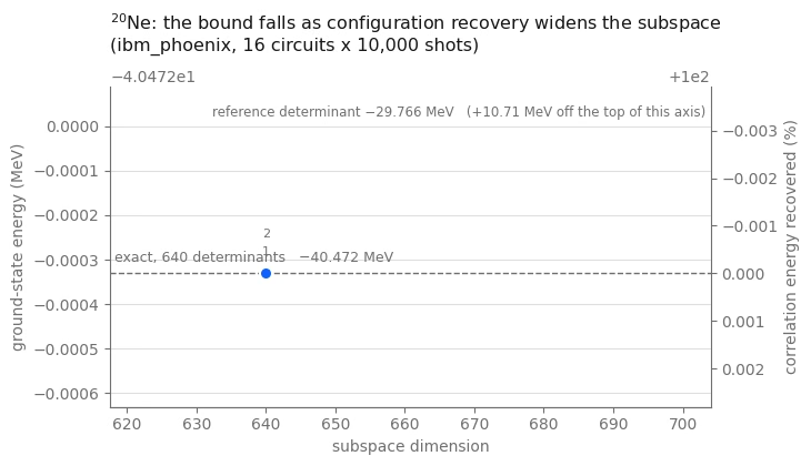
convergence_plot(
    result_sd["history"],
    E_REF_SD,
    E_EXACT_SD,
    f"$^{{20}}$Ne: the bound falls as configuration recovery widens the subspace\n"
    f"({backend.name}, {N_CIRCUITS} circuits x {SHOTS:,} shots)",
    full_dim=len(basis_exact_sd),
)
plt.show()

ตัวอย่างบนฮาร์ดแวร์ขนาดใหญ่

การขยายขนาดเปลี่ยนเพียงอินพุต ขั้นต่อไปจึงรวมสี่ขั้นตอนเป็นฟังก์ชันเดียว และรันสองครั้ง ทั้งสองครั้งบนรีจิสเตอร์ 40 qubit ใน shell $pf$ เหนือ core $^{40}\mathrm{Ca}$ ด้วยอันตรกิริยา GXPF1 [3]

การรันสองครั้งแสดงแง่มุมต่างกันของการขยายขนาด

• $^{44}\mathrm{Ti}$ โปรตอน valence สองตัวและนิวตรอน valence สองตัว มีฐาน 4,000 determinant รีจิสเตอร์คือ 40 qubit แต่ปัญหายังเล็กพอที่จะทำ diagonalization แบบแน่นอนบนแล็ปท็อป คุณจึงเปรียบเทียบผลจากฮาร์ดแวร์กับค่าอ้างอิงที่แน่นอนได้หลังเพิ่มขนาดรีจิสเตอร์

• $^{48}\mathrm{Cr}$ โปรตอน valence สี่ตัวและนิวตรอน valence สี่ตัว มี determinant ที่สมมาตรอนุญาต 1,963,461 ตัวใน 40 qubit เดียวกัน ตัวแก้แบบ dense ของบทเรียนไม่สามารถทำ diagonalization ปริภูมิเต็มนั้นได้ การรันจึงคืนค่า ขอบบนที่เข้มงวดและ determinant อ้างอิงที่มันปรับปรุงได้

สังเกตสองปริมาณตลอดการรันสองครั้ง สัดส่วนของพูลที่พอดีภายในงบประมาณ gate คงที่จะหดลงเมื่อพูลโตขึ้น และ pack_ensemble รายงานว่ารวมไว้เท่าใด ปริภูมิย่อยหยุดถูกจำกัดโดยการสุ่มและเริ่มถูกจำกัดโดย MAX_DIMENSION ซึ่งคือเมทริกซ์ ที่ใหญ่ที่สุดที่ตัวแก้คลาสสิกแบบ dense ที่นี่สร้างได้ ที่ขนาดนี้ การคำนวณ ระดับ production จะใช้ตัวแก้ selected configuration interaction (selected-CI)

รวม step 1–4

ฟังก์ชันต่อไปนี้เรียกขั้นตอนเดียวกับตัวอย่างเดินผ่าน ในลำดับเดียวกัน

def sqd_run(snt_file, n_protons, n_neutrons, name, exact=True):
    """The whole workflow for one nucleus.  Returns a record of every stage."""
    # -------------------------Step 1-------------------------
    ms = read_snt(DATA / snt_file, n_protons, n_neutrons)
    sp = m_scheme_states(ms)
    inter = Interaction(ms, sp)
    if sum(1 for s in sp if s.tz == -1) * 2 != len(sp):
        raise ValueError(
            f"{name}: post-selection needs equal proton and neutron state counts"
        )
    reference = reference_determinant(sp, inter, n_protons, n_neutrons)
    e_ref = matrix_element(inter, reference, reference)

    raw = excitation_pool(sp, reference)
    ranked = rank_pool(
        inter, reference, [op for op in raw if conserves_symmetry(sp, op)]
    )
    print(
        f"{name}: {len(sp)} qubits, {n_protons}p + {n_neutrons}n, A = {ms.mass_number}"
    )
    print(
        f"  2p2h pool {len(raw)} raw -> {len(ranked)} symmetry-allowed; "
        f"reference energy {e_ref:.6f} MeV"
    )

    # -------------------------Step 2-------------------------
    costs = excitation_costs(len(sp), ranked, costing_manager)
    circuits, bins, isa = pack_to_budget(
        len(sp),
        reference,
        ranked,
        costs,
        DEPTH_BUDGET,
        N_CIRCUITS,
        pass_manager,
    )
    packed = sum(len(b) for b in bins)
    worst = max(two_qubit_depth(c) for c in isa)
    worst_count = max(two_qubit_count(c) for c in isa)
    print(
        f"  packed {packed} of {len(ranked)} excitations; worst circuit two-qubit depth "
        f"{worst}, {worst_count} two-qubit gates"
    )

    # -------------------------Step 3-------------------------
    # a unique tag per run, so the jobs are findable later
    bit_arrays = sample(isa, SHOTS, JOB_TAGS + [name])
    matrix, probabilities, shots = pool_samples(bit_arrays, sp)
    survival = float(
        probabilities[
            (matrix[:, len(sp) // 2 :].sum(axis=1) == n_protons)
            & (matrix[:, : len(sp) // 2].sum(axis=1) == n_neutrons)
        ].sum()
    )
    print(
        f"  {shots:,} shots -> {len(matrix):,} distinct bitstrings, "
        f"{survival:.1%} of shots with the right nucleon numbers"
    )
    if survival == 0.0:
        raise RuntimeError(
            f"{name}: no shot carried the right nucleon numbers"
        )

    # -------------------------Step 4-------------------------
    result = recovery_loop(
        inter,
        sp,
        matrix,
        probabilities,
        reference,
        n_protons,
        n_neutrons,
        max_iterations=4,
        max_dimension=MAX_DIMENSION,
        seed=42,
    )
    energy = result["energy"]

    full_dim = count_basis(sp, n_protons, n_neutrons)  # cheap, even when huge
    e_exact = None
    if exact:
        full = full_basis(sp, n_protons, n_neutrons)
        if len(full) != full_dim:
            raise AssertionError(
                f"{name}: counted {full_dim} determinants but enumerated "
                f"{len(full)}"
            )
        e_exact, _ = ground_state(inter, full)

    print(f"  reference {e_ref:11.6f} MeV     pooled SQD {energy:11.6f} MeV")
    if e_exact is not None:
        print(
            f"  exact     {e_exact:11.6f} MeV  (dimension {full_dim})  ->  "
            f"{100 * (energy - e_ref) / (e_exact - e_ref):.1f}% of the correlation energy"
        )
        if energy < e_exact - 1e-7:
            raise AssertionError(
                f"{name}: pooled SQD bound is below the exact energy"
            )
    else:
        print(
            f"  no exact reference: the symmetry-allowed basis is {full_dim:,} determinants"
        )
        print(
            f"  the bound captures {energy - e_ref:.6f} MeV of correlation energy"
        )
    print()

    return dict(
        name=name,
        qubits=len(sp),
        pool=len(ranked),
        packed=packed,
        two_qubit=worst,
        two_qubit_gates=worst_count,
        shots=shots,
        distinct=len(matrix),
        survival=survival,
        dimension=len(result["basis"]),
        full_dim=full_dim,
        e_ref=e_ref,
        e_sqd=energy,
        e_exact=e_exact,
        history=result["history"],
        # the subspace and its eigenvector cannot be reconstructed from the summary --
        # they depend on the sampled shots -- so keep them for the scaling analysis
        interaction=inter,
        states=sp,
        reference=reference,
        ranked=ranked,
        basis=result["basis"],
        vector=result["vector"],
    )

pretty = {"20Ne": "$^{20}$Ne", "44Ti": "$^{44}$Ti", "48Cr": "$^{48}$Cr"}

small_scale = dict(
    name="20Ne",
    qubits=len(sp_sd),
    pool=len(ranked_sd),
    packed=PACKED_SD,
    two_qubit=worst_sd,
    two_qubit_gates=worst_count_sd,
    shots=shots_sd,
    distinct=len(matrix_sd),
    survival=shot_survival_sd,
    dimension=len(result_sd["basis"]),
    full_dim=len(basis_exact_sd),
    e_ref=E_REF_SD,
    e_sqd=E_SQD_SD,
    e_exact=E_EXACT_SD,
    history=result_sd["history"],
    interaction=inter_sd,
    states=sp_sd,
    reference=occ_sd,
    ranked=ranked_sd,
    basis=result_sd["basis"],
    vector=result_sd["vector"],
)

$^{44}\mathrm{Ti}$: เวิร์กโฟลว์เดียวกันบนรีจิสเตอร์ 40 qubit

shell $pf$ เหนือ $^{40}\mathrm{Ca}$ มีสี่ orbital ต่อชนิดและ 20 substate แม่เหล็กต่อชนิด ดังนั้นรีจิสเตอร์คือ 40 qubit โปรตอน valence สองตัวและนิวตรอน valence สองตัวสร้างเป็น $^{44}\mathrm{Ti}$ ที่มี determinant ที่สมมาตรอนุญาต 4,000 ตัว — ราวหกเท่าของฐาน $^{20}\mathrm{Ne}$ โดยใช้ 40 qubit แทน 24

นี่คือตัวอย่างที่ใหญ่กว่าในสองตัวอย่างที่โน้ตบุ๊กแก้ได้อย่างแน่นอน คุณจึงเปรียบเทียบ ผลจากฮาร์ดแวร์กับค่าอ้างอิงที่แน่นอนได้

large_scale_verified = sqd_run("gxpf1.snt", 2, 2, "44Ti", exact=True)

44Ti: 40 qubits, 2p + 2n, A = 44
  2p2h pool 1602 raw -> 174 symmetry-allowed; reference energy -44.309387 MeV
  packed 96 of 174 excitations; worst circuit two-qubit depth 272, 285 two-qubit gates
job dap31a02fm4c73f67dp0: 16 circuits x 10,000 shots on ibm_phoenix
  160,000 shots -> 48,170 distinct bitstrings, 18.6% of shots with the right nucleon numbers
  iteration 1: 187 proton x 189 neutron halves -> dimension 3891, E = -47.849086 MeV
  iteration 2: 190 proton x 190 neutron halves -> dimension 4000, E = -47.876666 MeV
  iteration 3: 190 proton x 190 neutron halves -> dimension 4000, E = -47.876666 MeV
  reference  -44.309387 MeV     pooled SQD  -47.876666 MeV
  exact      -47.876666 MeV  (dimension 4000)  ->  100.0% of the correlation energy

$^{48}\mathrm{Cr}$: เกินขีดความสามารถ exact-diagonalization ของบทเรียน

การเพิ่มโปรตอนสองตัวและนิวตรอนสองตัวใช้รีจิสเตอร์ 40 qubit เดิม (4, 4 สำหรับ $^{48}\mathrm{Cr}$) และเพิ่มขนาดฐานขึ้นราว 491 เท่า เป็น 1,963,461 determinant ที่สมมาตรอนุญาต เมทริกซ์นั้นใหญ่เกินกว่าที่บทเรียนนี้จะสร้างได้ไกลมาก ดังนั้น exact=False จึงไม่มีพลังงานอ้างอิงที่แน่นอน มีเพียงขอบ variational และ determinant อ้างอิงที่มันปรับปรุงได้

สองสิ่งเปลี่ยนไปที่ขนาดนี้ และเห็นได้ทั้งคู่ในผลลัพธ์ที่พิมพ์ออกมา พูลเติบโตเป็นการกระตุ้น (excitation) ที่อนุญาตหลายร้อยรายการ ดังนั้นงบประมาณ gate ที่กำหนดไว้จึงครอบคลุมเพียงส่วนน้อยของพูล ไม่ใช่ทั้งหมด นอกจากนี้ ปริภูมิย่อยผลคูณที่ตัวอย่างครอบคลุมยังมีขนาดใหญ่กว่า MAX_DIMENSION ตัวแก้แบบ dense จึงตัดปริภูมิย่อยนั้นตามน้ำหนักของตัวอย่าง ขอบเขตยังคงเข้มงวด แต่อาจแม่นยำน้อยกว่าขอบเขตที่ คำนวณจากการจัดเรียงที่สุ่มได้ทั้งหมด การคำนวณจริงในงานผลิตควรเก็บตัวอย่างไว้ และใช้ตัวแก้ที่รองรับปริภูมิย่อยขนาดใหญ่กว่านี้

large_scale_unverified = sqd_run("gxpf1.snt", 4, 4, "48Cr", exact=False)

48Cr: 40 qubits, 4p + 4n, A = 48
  2p2h pool 5536 raw -> 582 symmetry-allowed; reference energy -93.041237 MeV
  packed 96 of 582 excitations; worst circuit two-qubit depth 224, 279 two-qubit gates
job dap32a02fm4c73f67eog: 16 circuits x 10,000 shots on ibm_phoenix
  160,000 shots -> 55,436 distinct bitstrings, 18.6% of shots with the right nucleon numbers
  iteration 1: 223 proton x 223 neutron halves -> dimension 3977, E = -96.481598 MeV
  iteration 2: 223 proton x 223 neutron halves -> dimension 3977, E = -96.481598 MeV
  reference  -93.041237 MeV     pooled SQD  -96.481598 MeV
  no exact reference: the symmetry-allowed basis is 1,963,461 determinants
  the bound captures -3.440361 MeV of correlation energy

ประเมินผลลัพธ์โดยไม่มีค่าอ้างอิงที่แน่นอน

การรัน $^{48}\mathrm{Cr}$ ไม่มีค่าอ้างอิงที่แน่นอนภายในบทเรียนนี้ ให้ใช้ตัวอย่างที่มีอยู่ เพื่อประเมินการลู่เข้า และเปรียบเทียบกับ baseline การเลือกแบบคลาสสิก โดยไม่ต้องใช้เวลา QPU เพิ่มเติม หรือการทำ diagonalization เต็มปริภูมิ

ลู่เข้าแล้วหรือยัง? จัดเรียง determinant ที่เก็บไว้ใหม่ตามน้ำหนักใน eigenvector ที่ลู่เข้าแล้ว ปริภูมิย่อยจะกลายเป็นแบบ ซ้อนกัน การทำ diagonalization บล็อก $d \times d$ นำหน้าสำหรับลำดับค่า $d$ จะแสดงการลดลงของขอบเขตข้ามขนาดปริภูมิย่อยสองระดับของหลักสิบ ถ้ายังลดลงชันที่ $d$ ใหญ่สุด แสดงว่าขีดจำกัดมิติของตัวแก้คลาสสิกคือข้อจำกัดหลัก และ MAX_DIMENSION คือ พารามิเตอร์ที่ควรเพิ่ม ถ้ากราฟราบแล้ว การเพิ่ม determinant ที่เก็บไว้อีกจะช่วยได้น้อย ความก้าวหน้าต่อไปอาจต้องสุ่มการจัดเรียงเพิ่มเติม Hamiltonian ถูกสร้างครั้งเดียวที่ขนาดเต็ม และแต่ละขั้นเป็นบล็อกหลักของมัน ดังนั้นการกวาดทั้งหมด ใช้การสร้างเมทริกซ์เพียงครั้งเดียว ไม่ใช่หนึ่งครั้งต่อขั้น

การสุ่มตัวอย่างแบบควอนตัมเทียบกับการเลือกแบบคลาสสิกเป็นอย่างไร? เปรียบเทียบกับปริภูมิย่อยที่ มีขนาดเท่ากันซึ่งเลือกด้วยขั้นตอนการเลือกแบบคลาสสิก: นำพูลที่จัดอันดับด้วยทฤษฎีการรบกวนตามลำดับคะแนนมา ขยายปริภูมิย่อยผลคูณให้มีมิติเท่ากัน แล้วทำ diagonalization อันนั้นแทน เส้นโค้งทั้งสองเป็น ขอบเขตบนที่เข้มงวดของ Hamiltonian เดียวกัน ดังนั้นเส้นที่ต่ำกว่าที่มิติเท่ากันคือเส้นที่เลือก determinant ได้ดีกว่า การเปรียบเทียบนี้ตัดสินว่าการสุ่มตัวอย่างบนฮาร์ดแวร์ช่วยปรับปรุงการประมาณพลังงาน เมื่อเทียบกับ baseline แบบคลาสสิกนี้หรือไม่

ปริภูมิย่อยนี้ไม่ได้ถูกเลือกสำหรับสถานะกระตุ้น การกู้คืนการจัดเรียง (configuration recovery) นำทางปริภูมิย่อย ด้วยการครอบครองของสถานะพื้น ดังนั้นค่าเฉพาะที่สูงกว่าจึงอยู่ห่างจากการลู่เข้ามากกว่า ค่าต่ำสุด และพลังงานกระตุ้นแรกจึงออกมาสูงกว่า $2^+$ ที่วัดได้มาก การจะไปถึงสถานะกระตุ้นได้อย่างเหมาะสม ต้องใช้ปริภูมิย่อยที่เลือกมาสำหรับสถานะเหล่านั้นโดยเฉพาะ

def subspace_scaling(
    inter, basis, vector, points=18, smallest=32, largest=None
):
    """Nested Rayleigh-Ritz sweep: the lowest eigenvalue of the leading d x d block, for a ladder of d.

    Reordering the basis by descending weight in the converged eigenvector makes every subspace in
    the ladder a subset of the next, so the energies fall monotonically and each one is a valid
    variational bound.  H is built once at full size; each rung is a principal block.
    """
    order = np.argsort(-(np.abs(vector) ** 2))
    ordered = [basis[i] for i in order]
    weights = (np.abs(vector) ** 2)[order]
    if (
        largest is not None
    ):  # cap the ladder so two subspaces end at a common dimension
        ordered, weights = ordered[:largest], weights[:largest]
    H = subspace_hamiltonian(inter, ordered)
    dimensions = np.unique(
        np.geomspace(smallest, len(ordered), points).astype(int)
    )
    rows = [
        (
            int(d),
            float(
                eigh(H[:d, :d], eigvals_only=True, subset_by_index=[0, 0])[0]
            ),
        )
        for d in dimensions
    ]
    return rows, np.cumsum(weights)

def classical_selection(
    inter, sp, reference, ranked, target, n_protons, n_neutrons
):
    """The subspace classical perturbative ranking would pick, grown to `target` dimension.

    Same product construction as the sampled subspace, and the same truncation discipline -- half
    configurations are offered to `grow_subspace` in order of importance and it takes as many as
    fit.  The only difference from the sampled path is where the ordering comes from: PT2 score
    here, measured sampling weight there.  So the comparison isolates *which determinants got
    chosen* and nothing else.

    Truncating by any other rule would not be a fair baseline.  Slicing an arbitrarily ordered
    list, for instance, keeps determinants by accident rather than by importance and makes the
    classical subspace look worse than classical selection really is.
    """
    p_ref = tuple(i for i in reference if sp[i].tz == -1)
    n_ref = tuple(i for i in reference if sp[i].tz == +1)
    reached = {reference}
    proton_order, neutron_order = [p_ref], [n_ref]
    seen_p, seen_n = {p_ref}, {n_ref}
    product_budget = 4 * target

    for op, _, _ in ranked:  # ranked is already in descending PT2 score
        h1, h2, v1, v2 = op
        fresh = {
            tuple(sorted(set(d) - {h1, h2} | {v1, v2}))
            for d in reached
            if {h1, h2} <= set(d) and not {v1, v2} & set(d)
        }
        reached |= fresh
        for det in fresh:  # first appearance fixes a half's rank
            half_p = tuple(i for i in det if sp[i].tz == -1)
            half_n = tuple(i for i in det if sp[i].tz == +1)
            if half_p not in seen_p:
                seen_p.add(half_p)
                proton_order.append(half_p)
            if half_n not in seen_n:
                seen_n.add(half_n)
                neutron_order.append(half_n)
        if len(proton_order) * len(neutron_order) > product_budget:
            # Half-configuration products over-count the subspace, because only the
            # symmetry-allowed ones survive `product_subspace`.  Stopping on the product
            # count alone can therefore leave the basis far short of `target`, so check
            # the dimension actually realized and widen the budget if it falls short.
            trial, _, _ = grow_subspace(
                sp,
                [p_ref],
                [n_ref],
                proton_order,
                neutron_order,
                n_protons,
                n_neutrons,
                max_dimension=target,
            )
            if len(trial) >= target:
                break
            product_budget *= 2

    basis, _, _ = grow_subspace(
        sp,
        [p_ref],
        [n_ref],
        proton_order,
        neutron_order,
        n_protons,
        n_neutrons,
        max_dimension=target,
    )
    return basis

run = large_scale_unverified
if "basis" not in run:
    raise RuntimeError(
        "this cell needs the subspace and eigenvector that sqd_run now returns; "
        "re-run the sqd_run definition and the 48Cr cell"
    )

print(
    f"{run['name']}: sweeping nested subspaces of the sampled basis "
    f"(dimension {run['dimension']})"
)
sampled_rows, cumulative = subspace_scaling(
    run["interaction"], run["basis"], run["vector"]
)

print(
    f"{run['name']}: building the classically selected subspace at the same dimension"
)
classical_basis = classical_selection(
    run["interaction"],
    run["states"],
    run["reference"],
    run["ranked"],
    run["dimension"],
    4,
    4,
)
# Both subspaces must be scored at the same dimension.  Symmetry filtering can still leave
# the classical construction short of the target when the ranked pool runs out, so take the
# dimension both actually reach, cap both ladders there, and verify they agree.
common_dim = min(sampled_rows[-1][0], len(classical_basis))
if common_dim < sampled_rows[-1][0]:
    sampled_rows, _ = subspace_scaling(
        run["interaction"], run["basis"], run["vector"], largest=common_dim
    )
classical_rows, _ = subspace_scaling(
    run["interaction"],
    classical_basis,
    ground_state(run["interaction"], classical_basis)[1],
    largest=common_dim,
)
if sampled_rows[-1][0] != classical_rows[-1][0]:
    raise RuntimeError(
        f"comparison dimensions differ: sampled {sampled_rows[-1][0]}, "
        f"classical {classical_rows[-1][0]}"
    )

advantage = sampled_rows[-1][1] - classical_rows[-1][1]
direction = "lower" if advantage < 0 else "higher"
verdict = "beats" if advantage < 0 else "does not beat"
descent = next(
    e for d, e in reversed(sampled_rows) if d <= sampled_rows[-1][0] / 2
)
for fraction in (0.90, 0.99):
    count = int(np.searchsorted(cumulative, fraction) + 1)
    print(
        f"  {fraction:.0%} of the eigenvector norm sits on {count} determinants "
        f"({count / run['full_dim']:.1e} of the {run['full_dim']:,}-determinant space)"
    )
print(
    f"  bound still falling {1000 * (sampled_rows[-1][1] - descent):+.1f} keV "
    f"over the last doubling of dimension"
)
print(
    f"  sampled {sampled_rows[-1][1]:.6f} MeV vs classically selected "
    f"{classical_rows[-1][1]:.6f} MeV at a verified common dimension of "
    f"{classical_rows[-1][0]:,}"
)
print(
    f"  -> the sampled subspace is {abs(advantage) * 1000:.0f} keV {direction}"
)

48Cr: sweeping nested subspaces of the sampled basis (dimension 3977)
48Cr: building the classically selected subspace at the same dimension
  90% of the eigenvector norm sits on 107 determinants (5.4e-05 of the 1,963,461-determinant space)
  99% of the eigenvector norm sits on 593 determinants (3.0e-04 of the 1,963,461-determinant space)
  bound still falling -15.6 keV over the last doubling of dimension
  sampled -96.481598 MeV vs classically selected -95.314510 MeV at a verified common dimension of 3,957
  -> the sampled subspace is 1167 keV lower

fig, axes = plt.subplots(1, 2, figsize=(11.2, 4.0), facecolor=SURFACE)

# left: two nested convergence curves on the same axes
ax = axes[0]
ax.set_facecolor(SURFACE)
ax.plot(
    [d for d, _ in sampled_rows],
    [e for _, e in sampled_rows],
    "-o",
    color=SERIES,
    linewidth=2,
    markersize=5,
    markeredgecolor=SURFACE,
    markeredgewidth=1,
    zorder=4,
    label="sampled on the QPU",
)
ax.plot(
    [d for d, _ in classical_rows],
    [e for _, e in classical_rows],
    "--s",
    color=MUTED,
    linewidth=1.6,
    markersize=4,
    markeredgecolor=SURFACE,
    markeredgewidth=1,
    zorder=3,
    label="classically selected, same size",
)
ax.axhline(run["e_ref"], color=RULE, linestyle=":", linewidth=1.2, zorder=1)
ax.annotate(
    f"reference determinant {run['e_ref']:.2f} MeV".replace("-", "\u2212"),
    xy=(sampled_rows[-1][0], run["e_ref"]),
    xytext=(-2, 4),
    textcoords="offset points",
    ha="right",
    va="bottom",
    color=MUTED,
    fontsize=8,
)

# mark the gap between the two curves at the largest dimension, not either curve alone
edge = sampled_rows[-1][0]
ax.plot(
    [edge, edge],
    [classical_rows[-1][1], sampled_rows[-1][1]],
    "-",
    color=SERIES,
    linewidth=1.0,
    alpha=0.7,
    zorder=2,
)
ax.annotate(
    f"{abs(advantage) * 1000:.0f} keV {direction}\nat equal dimension",
    xy=(edge, 0.5 * (classical_rows[-1][1] + sampled_rows[-1][1])),
    xytext=(-8, 0),
    textcoords="offset points",
    ha="right",
    va="center",
    color=SERIES,
    fontsize=8.5,
)

ax.set_xscale("log")
ax.set_xlim(sampled_rows[0][0] * 0.75, edge * 1.5)
ax.set_xlabel("subspace dimension", color=MUTED)
ax.set_ylabel("variational upper bound (MeV)", color=MUTED)
ax.set_title(
    f"{pretty[run['name']]}: the bound, and the subspace it {verdict}",
    color=INK,
    fontsize=11,
    loc="left",
    pad=10,
)
legend = ax.legend(frameon=False, fontsize=8.5, loc="lower left")
for text in legend.get_texts():
    text.set_color(MUTED)

# right: why a few thousand determinants can bound two million
ax = axes[1]
ax.set_facecolor(SURFACE)
ranks = np.arange(1, len(cumulative) + 1)
ax.plot(ranks, 100 * cumulative, "-", color=DEEP, linewidth=2, zorder=3)
for fraction, style, label_y in ((0.90, ":", 46), (0.99, "--", 24)):
    count = int(np.searchsorted(cumulative, fraction) + 1)
    ax.axvline(count, color=MUTED, linestyle=style, linewidth=1, zorder=1)
    ax.annotate(
        f"{fraction:.0%} of the norm\non {count} determinants",
        xy=(count, label_y),
        xytext=(7, 0),
        textcoords="offset points",
        ha="left",
        va="center",
        color=MUTED,
        fontsize=8.5,
    )
ax.set_xscale("log")
ax.set_xlim(0.8, len(cumulative) * 2.6)
ax.set_ylim(0, 104)
ax.set_xlabel("determinants, ordered by weight", color=MUTED)
ax.set_ylabel("cumulative share of the eigenvector (%)", color=MUTED)
ax.set_title(
    f"Sparsity: {run['full_dim']:,} determinants in the sector",
    color=INK,
    fontsize=11,
    loc="left",
    pad=10,
)

for ax in axes:
    ax.grid(axis="y", color=RULE, alpha=0.55)
    ax.tick_params(colors=MUTED, labelsize=8.5)
    for side in ("top", "right"):
        ax.spines[side].set_visible(False)
    for side in ("bottom", "left"):
        ax.spines[side].set_color(MUTED)
fig.tight_layout()
plt.show()

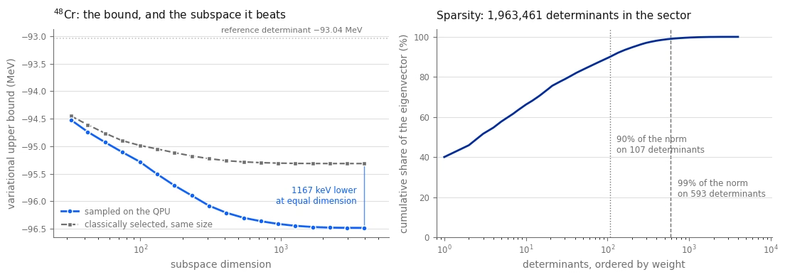
เปรียบเทียบการรันทั้งสามครั้ง

พลังงานสัมบูรณ์ไม่สามารถเปรียบเทียบข้ามนิวเคลียสและอันตรกิริยาที่ต่างกันได้ จึงควรโฟกัสที่สัดส่วนของพลังงานสหสัมพันธ์ที่กู้คืนได้ในแต่ละการรัน ในกรณีที่มีค่าอ้างอิงที่แน่นอน และเปรียบเทียบความลึกของ circuit กับสัดส่วนของ shot ที่ถูกทิ้งด้วย

runs = [small_scale, large_scale_verified, large_scale_unverified]

print(
    f"{'run':>6}  {'qubits':>6}  {'pool':>9}  {'2q depth':>8}  {'2q gates':>8}  "
    f"{'shots kept':>10}  {'dim':>6}  {'of':>9}  {'% corr':>7}"
)
for r in runs:
    fraction = (
        "--"
        if r["e_exact"] is None
        else f"{100 * (r['e_sqd'] - r['e_ref']) / (r['e_exact'] - r['e_ref']):.1f}%"
    )
    coverage = "{}/{}".format(r["packed"], r["pool"])
    print(
        f"{r['name']:>6}  {r['qubits']:>6}  {coverage:>9}  "
        f"{r['two_qubit']:>8}  {r['two_qubit_gates']:>8}  {r['survival']:>9.1%}  "
        f"{r['dimension']:>6}  {(r['full_dim'] or 0):>9,}  {fraction:>7}"
    )

print()
for r in runs:
    exact = (
        f"exact {r['e_exact']:11.6f}"
        if r["e_exact"] is not None
        else "exact  unavailable"
    )
    print(
        f"{r['name']:>6}   reference {r['e_ref']:11.6f}   pooled SQD {r['e_sqd']:11.6f}   {exact} MeV"
    )

run  qubits       pool  2q depth  2q gates  shots kept     dim         of   % corr
  20Ne      24      78/78       228       234      31.5%     640        640   100.0%
  44Ti      40     96/174       272       285      18.6%    4000      4,000   100.0%
  48Cr      40     96/582       224       279      18.6%    3977  1,963,461       --

  20Ne   reference  -29.765549   pooled SQD  -40.472331   exact  -40.472331 MeV
  44Ti   reference  -44.309387   pooled SQD  -47.876666   exact  -47.876666 MeV
  48Cr   reference  -93.041237   pooled SQD  -96.481598   exact  unavailable MeV

# Left: how much of the correlation energy was recovered, where the exact answer is known.
# Right: the bound itself for the run that has nothing to score against.
scored = [r for r in runs if r["e_exact"] is not None]

fig, ax = plt.subplots(figsize=(6.4, 3.9), facecolor=SURFACE)
ax.set_facecolor(SURFACE)
labels = [
    f"{pretty[r['name']]}\n{r['qubits']} qubits\n{r['full_dim']:,} determinants"
    for r in scored
]
fractions = [
    100 * (r["e_sqd"] - r["e_ref"]) / (r["e_exact"] - r["e_ref"])
    for r in scored
]
shades = [SERIES, DEEP, PURPLE]
bars = ax.bar(
    labels, fractions, width=0.46, color=shades[: len(scored)], zorder=3
)
for bar, fraction, r in zip(bars, fractions, scored):
    ax.annotate(
        f"{fraction:.1f}%",
        xy=(bar.get_x() + bar.get_width() / 2, fraction),
        xytext=(0, 5),
        textcoords="offset points",
        ha="center",
        va="bottom",
        color=INK,
        fontsize=10,
    )
    ax.annotate(
        f"dim {r['dimension']:,}",
        xy=(bar.get_x() + bar.get_width() / 2, 3),
        ha="center",
        va="bottom",
        color=SURFACE,
        fontsize=8.5,
    )
ax.axhline(100, color=MUTED, linestyle="--", linewidth=1, zorder=1)
ax.annotate(
    "exact diagonalization",
    xy=(-0.45, 100),
    xytext=(0, 4),
    textcoords="offset points",
    ha="left",
    va="bottom",
    color=MUTED,
    fontsize=8.5,
)
ax.set_ylim(0, 118)
ax.set_ylabel("correlation energy recovered (%)", color=MUTED)
ax.set_title(
    f"Where the exact answer is known ({backend.name})",
    color=INK,
    fontsize=11,
    loc="left",
    pad=10,
)
ax.grid(axis="y", color=RULE, alpha=0.55)
ax.tick_params(colors=MUTED, labelsize=8.5)
for side in ("top", "right"):
    ax.spines[side].set_visible(False)
for side in ("bottom", "left"):
    ax.spines[side].set_color(MUTED)
fig.tight_layout()
plt.show()

# the same convergence view as the walkthrough, for the run with no exact reference
convergence_plot(
    large_scale_unverified["history"],
    large_scale_unverified["e_ref"],
    None,
    f"{pretty[large_scale_unverified['name']]}: "
    f"{large_scale_unverified['full_dim']:,} determinants, no exact answer to score against\n"
    f"({backend.name}, {N_CIRCUITS} circuits x {SHOTS:,} shots)",
    colour=DEEP,
)
plt.show()

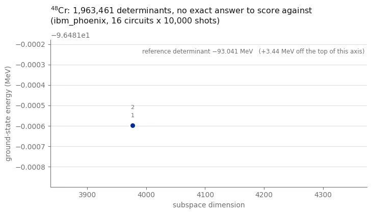
สรุป

เวิร์กโฟลว์เดียวที่ไม่เปลี่ยนแปลงนอกจากอินพุต ถูกรันบน QPU ที่ปัญหาสามขนาด: ปัญหา 24 qubit ที่ตรวจสอบได้อย่างแน่นอน ปัญหา 40 qubit ที่ยังตรวจสอบได้อย่างแน่นอน และปัญหา 40 qubit ที่มี basis state เกือบสองล้านสถานะ เกินความสามารถของ exact diagonalization ในบทเรียนนี้

การรันทั้งสามครั้งแสดงประเด็นต่อไปนี้:

• ขั้นตอนควอนตัมต้องเพียงเสนอ determinant circuit ถูกกำหนดตายตัว เริ่มจาก ทฤษฎีการรบกวนอันดับสอง และไม่เคยถูกปรับให้เหมาะสม ไม่มีสิ่งใดในเวิร์กโฟลว์ที่ต้องการให้แอมพลิจูดของมัน แม่นยำ ขอเพียง support ของมันมีประโยชน์ Classical diagonalization ในปริภูมิย่อยที่เลือกให้ ขอบเขตบนแบบ variational แม้ว่าขอบเขตนี้จะแปรผันตามการจัดเรียงที่สุ่มได้

• Qubit excitation ลดความลึกของ circuit เนื่องจากมีเพียง support ที่สำคัญ บล็อก fermionic excitation จึงแทนที่ด้วย qubit excitation ได้ ซึ่งต้นทุนไม่เพิ่มตามระยะห่างระหว่าง ออร์บิทัลที่มันเชื่อม ขั้นที่ 2 วัดการประหยัดนี้บน backend จริง ซึ่งเป็น ความต่างระหว่าง circuit ที่พอดีอยู่ในช่วง coherence ได้สบาย กับอันที่ไม่พอดี

• Configuration recovery นำตัวอย่างที่มีสัญญาณรบกวนกลับมาใช้ใหม่ ทุก shot ที่มีจำนวนโปรตอนหรือนิวตรอนผิดจะถูกซ่อมแซม เทียบกับค่าประมาณการครอบครองปัจจุบัน แทนที่จะถูกทิ้ง และแต่ละครึ่งการจัดเรียงที่ซ่อมแล้ว อาจเพิ่มการจัดเรียงเข้าสู่ปริภูมิย่อย การขยายปริภูมิย่อยแบบ variational ไม่สามารถทำให้ค่าเฉพาะต่ำสุดสูงขึ้นได้ บทเรียนนี้สาธิต configuration recovery โดยใช้ตัวอย่างจากฮาร์ดแวร์

• ข้อจำกัดหลักเปลี่ยนไปเมื่อคุณขยายขนาด ที่ 24 qubit ansatz เข้าถึงคำตอบที่แน่นอนได้ และมีเพียงการสุ่มตัวอย่างที่ขวางอยู่ ที่ 40 qubit กับนิวคลีออนวาเลนซ์สี่ตัวต่อชนิด งบประมาณ gate ครอบคลุมเพียงส่วนน้อยของพูล และตัวแก้คลาสสิกแบบ dense จำกัดปริภูมิย่อย การรู้ว่า ในสามอย่างนี้อะไรที่จำกัดคุณอยู่ คือทักษะเชิงปฏิบัติที่เวิร์กโฟลว์นี้สอน

ขั้นตอนถัดไป

คำแนะนำ

สำรวจแหล่งข้อมูลที่เกี่ยวข้องเหล่านี้:

• Sample-based quantum diagonalization ของ chemistry Hamiltonian: อัลกอริทึมเดียวกันที่ใช้กับโครงสร้างอิเล็กตรอน โดยใช้ตัวแก้ selected-CI ของ SQD addon

• เอกสาร SQD addon: ยูทิลิตีสำหรับ post-selection, subsampling และ configuration recovery

• Quantum diagonalization algorithms: คอร์สเต็มเกี่ยวกับ subspace diagonalization รวมถึงรูปแบบ Krylov

• Introduction to transpilation: ตัวเลือก pass-manager ที่สำคัญเมื่อ circuit ถูกครอบงำด้วย gate สอง qubit

• Execution modes: สำรวจ batch mode สำหรับการจัดตารางงานที่เป็นอิสระต่อกัน

ส่วนขยายที่ควรพิจารณา

• แทนที่ตัวแก้แบบ dense MAX_DIMENSION คือเพดานของทุกอย่างที่สเกล $^{48}\mathrm{Cr}$ และ np.linalg.eigh บนเมทริกซ์ dense คือสาเหตุ การสร้าง Hamiltonian ที่ฉายเดียวกัน เป็นเมทริกซ์แบบ sparse และใช้ eigensolver แบบวนซ้ำ เช่น scipy.sparse.linalg.eigsh หรือตัวแก้ Davidson หรือ selected-CI ที่ออกแบบสำหรับอันตรกิริยาสองวัตถุของนิวเคลียส อาจรองรับปริภูมิย่อยที่ใหญ่ขึ้นได้ ขีดจำกัดเชิงปฏิบัติขึ้นอยู่กับความ sparse ของเมทริกซ์ หน่วยความจำที่มี และการลู่เข้าของตัวแก้ และบทเรียนนี้ไม่ได้ benchmark ส่วนขยายนั้น qiskit_addon_sqd.fermion.solve_sci ของ SQD addon ไม่ใช่ตัวแทนที่ใช้แทนกันได้ทันที: มันห่อตัวแก้ โครงสร้างอิเล็กทรอนิกส์ และคาดหวังปริพันธ์หนึ่งและสองวัตถุในรูปแบบนั้น ดังนั้นโครงสร้างผลคูณ โปรตอน $\times$ นิวตรอนที่ใช้ร่วมกันจึงไม่เพียงพอด้วยตัวมันเอง การใช้มันหมายถึงการแมป อันตรกิริยา shell-model ของสมการ (1) ไปเป็นปริพันธ์เหล่านั้น และตรวจสอบผลลัพธ์เทียบกับ พลังงานที่แน่นอนที่โน้ตบุ๊กนี้คำนวณไว้แล้ว

• เพิ่ม batching และ subsampling เวิร์กโฟลว์ pooled SQD ที่ตีพิมพ์ทำ diagonalization หลาย subsample อิสระต่อรอบ และเก็บอันที่ดีที่สุด บทเรียนนี้ใช้หนึ่ง batch ต่อรอบ ซึ่ง ไม่เป็นอันตรายต่อขอบเขต variational แต่ไม่ให้ข้อมูลความแปรปรวนที่บ่งชี้ว่าการเพิ่ม shot จะช่วยหรือไม่

• สถานะกระตุ้นและเซกเตอร์อื่น ค่าเฉพาะที่สูงกว่าของ Hamiltonian ปริภูมิย่อยแต่ละอันเป็นขอบเขต บนของสถานะกระตุ้นในเซกเตอร์สมมาตรเดียวกัน และการรันที่ $M_J \neq 0$ ไปถึง เซกเตอร์อื่นได้ การตรวจสอบ $2^+$ ในขั้นที่ 1 เป็นครึ่งหนึ่งของการคำนวณนี้แล้ว

• ปริภูมิโมเดลข้ามเชลล์ พาริตีถูกสอดคล้องโดยอัตโนมัติภายในเมเจอร์เชลล์เดียว ซึ่ง เป็นเหตุผลที่มันไม่ทำงานอะไรที่นี่ ปริภูมิ $sd$-$pf$ ผสมพาริตี $\ell$ ทำให้พาริตีเป็นข้อจำกัด ที่สี่อย่างแท้จริง ซึ่งทั้งการซ่อม Hamming-weight ของ SQD และการสร้างผลคูณ ก็ไม่อาจจับได้ด้วยตัวเอง

• นิวเคลียสมวลคี่ reference_determinant ต้องการจำนวนวาเลนซ์เป็นคู่ในแต่ละชนิด เพราะการเติมเป็นคู่ที่กลับเวลาคือสิ่งที่บังคับให้ $M_J = 0$ นิวเคลียสคี่ต้องใช้ เป้าหมาย $M_J$ ครึ่งจำนวนเต็มและ reference ที่ไม่เป็นคู่

ภาคผนวก

ส่วนนี้อธิบายเหตุผลเบื้องหลังตัวช่วยที่แนะนำในส่วน Setup

ทำไมการปรับสเกลตามมวลจึงไม่ใช่ทางเลือก

อันตรกิริยา shell-model เชิงประจักษ์ถูกฟิตที่มวลหนึ่งและใช้ข้ามห่วงโซ่ไอโซโทป โดย สมาชิกเมทริกซ์สองวัตถุถูกปรับสเกลด้วย $(A/A_{\mathrm{ref}})^{p}$ ไฟล์อันตรกิริยาทั้งสองมี $p = -0.3$ โดย $A_{\mathrm{ref}} = 18$ สำหรับตระกูล USD และ $42$ สำหรับ GXPF1 ที่บรรทัดส่วนหัวสองวัตถุ ของไฟล์ .snt ตัวเลขสองตัวนั้นอยู่ในตำแหน่งที่ความถี่ออสซิลเลเตอร์และพลังงานแกนกลาง น่าจะอยู่ ทำให้อ่านผิดได้ง่าย การอ่านเลขชี้กำลังเป็นพลังงานแกนกลางคงที่จะเพิ่ม ออฟเซ็ตปลอมให้ทุกสมาชิกแนวทแยง และ ทำให้การปรับสเกลหายไป เปลี่ยนพลังงานสหสัมพันธ์ไป ไม่กี่เปอร์เซ็นต์ การตรวจสอบสมมาตรในขั้นที่ 1 ไม่ได้ยืนยันสเกลพลังงานด้วยตัวเอง การเปรียบเทียบ พลังงานกระตุ้น $2^+$ ที่วัดเป็น MeV กับการทดลองเป็นการตรวจสอบเพิ่มเติมสำหรับ การปรับสเกลตามมวล พลังงานกระตุ้นคือความต่างระหว่างระดับ จึงตรวจจับ ออฟเซ็ตคงที่ที่ใช้กับพลังงานทั้งหมดไม่ได้

ทำไมจึงหา reference ด้วยการค้นหาแทนการเติม

reference ที่ชัดเจนคือ determinant ที่เติมพลังงานอนุภาคเดี่ยวต่ำสุด แต่มันไม่ใช่ determinant พลังงานต่ำสุด เพราะแนวทแยงของสมการ (1) รวมเทอมสองวัตถุ $\sum_{i<j} \langle ij \| ij \rangle$ และอันตรกิริยาแบบ pairing ชอบอย่างมากให้ครอบครอง คู่ที่กลับเวลา $(+m_j, -m_j)$ ที่ $|m_j|$ ใหญ่ที่สุด ที่มี ในเชลล์ $sd$ นั่นคือ ความต่างระหว่างคู่ $m_j = \pm 1/2$ กับคู่ $m_j = \pm 5/2$ ของ $0d_{5/2}$ และมีค่า ประมาณ 1 MeV ในเชลล์ $pf$ มีค่าใกล้ 2 เพราะพลังงาน reference กำหนดศูนย์ของเมตริก "พลังงานสหสัมพันธ์ที่กู้คืนได้" การเลือกที่ไม่ดีจึงทำให้เมตริกนั้นพองเกินจริงและให้ จุดเริ่มต้นที่แม่นยำน้อยลง

การจำกัดเฉพาะการเติมเป็นคู่ทำให้การค้นหาแบบทั่วถึงมีต้นทุนต่ำ โดยมี $\binom{n_{\mathrm{pairs}}}{k}$ ตัวเลือกต่อ ชนิด (อย่างมากไม่กี่พัน) และรับประกัน $M_J = 0$ ในทุกกรณีของ บทเรียนนี้ที่ตรวจสอบเทียบกับการแจกแจงเต็มได้ การค้นหาคืนค่า determinant แนวทแยงต่ำสุดโดยรวม ซึ่งก็เป็นองค์ประกอบเดี่ยวที่ใหญ่ที่สุดของสถานะพื้นที่แน่นอนด้วย

ทำไมจึงใช้แอมพลิจูดอันดับหนึ่ง ไม่ใช่มุมสองระดับที่แน่นอน

การทำ diagonalization Hamiltonian $2 \times 2$ ในปริภูมิ $\{|\Phi_{\mathrm{ref}}\rangle, |\alpha\rangle\}$ ให้มุมผสม $\theta_{\mathrm{exact}} = \tfrac{1}{2}\arctan(2V/\Delta)$ ซึ่งอาจน่าเรียกว่าเป็นตัวเลือกที่ถูกต้อง สำหรับระดับคู่ที่ แยกโดด ใน ansatz นี้ บล็อก excitation หลายสิบบล็อกทำงาน ต่อเนื่องกันบน reference เดียวกัน ดังนั้นการปรับแต่งแต่ละบล็อกแยกกันไม่จำเป็นต้อง ปรับแต่ง circuit ประกอบให้เหมาะสม

บทบาทของ circuit เป็นตัวกำหนดการเลือกมุม เนื่องจาก $|\tfrac{1}{2}\arctan(2x)| \le |x|$ สำหรับทุก $x$ จริง มุมที่แน่นอนจึงมี ขนาด เล็กกว่า แอมพลิจูดอันดับหนึ่ง $t = V/\Delta$ เสมอ และทำให้เหลือแอมพลิจูด มากกว่า บน determinant อ้างอิงเสมอ circuit ที่เก็บแอมพลิจูดบน reference มากกว่าจะคืน reference บ่อยขึ้นและ determinant กระตุ้นที่ต่างกันน้อยลง สำหรับ pooled SQD ผลลัพธ์ที่มีประโยชน์ของแต่ละ shot คือ determinant ที่ขั้นตอนคลาสสิกยังไม่เคยเห็น ซึ่งเป็นเหตุผลที่บทเรียนนี้ใช้มุมที่ใหญ่กว่า ไม่มีมุมใดต้องแม่นยำ เพราะ classical diagonalization ทิ้งแอมพลิจูดของ circuit ทั้งหมดและคำนวณของตัวเองใหม่

ทำไม pooled SQD จึงใช้ qubit excitation ได้

fermionic excitation $T = a_{v_1}^\dagger a_{v_2}^\dagger a_{h_2} a_{h_1}$ แมปภายใต้ Jordan-Wigner เป็น Pauli string แปดตัว แต่ละตัวมีตัวดำเนินการ $Z$ บนทุก qubit ระหว่างดัชนี นอกสุด string เหล่านั้นเข้ารหัสเครื่องหมายแบบ fermionic และต้นทุนเพิ่มตามช่วงที่ครอบ ซึ่งสำหรับ excitation โปรตอน-นิวตรอนคือทั้งรีจิสเตอร์

การลบมันออกให้ตัวดำเนินการ qubit-excitation ของ Yordanov et al. [5] ซึ่งเป็น ตัวดำเนินการที่ต่างออกไป: สถานะที่มันเตรียมต่างจากแบบ fermionic ใน เครื่องหมาย ของ แอมพลิจูด และการแจกแจงการสุ่มตัวอย่างทั้งสองอาจต่างกันมาก สิ่งที่มันไม่เปลี่ยนคือ determinant ใดมีแอมพลิจูดไม่เป็นศูนย์ เพราะแต่ละบล็อกยังคงหมุนภายในปริภูมิสองมิติเดียวกัน $\{|d\rangle, |d'\rangle\}$ สำหรับทุก determinant $d$ ที่มันกระทำ และยัง อนุรักษ์จำนวนนิวคลีออนทั้งสองชนิด $M_J$ และพาริตีได้อย่างแน่นอน ดังนั้นเซตของ determinant ที่เข้าถึงได้ จึงเหมือนกัน และเซตที่เข้าถึงได้เป็นสิ่งเดียวที่ pooled SQD ใช้ การ diagonalization แบบคลาสสิกกำหนดแอมพลิจูดของตัวเองไม่ว่ากรณีใด ขั้นที่ 2 ตรวจสอบข้ออ้าง support เหมือนกันบน ตัวดำเนินการจริงจากพูล และวัดว่าการแทนที่ประหยัดได้เท่าไร

ข้อจำกัดคือ น้ำหนัก การสุ่มตัวอย่างต่างกัน ดังนั้นการสร้างทั้งสองแบบจะไม่ค้นพบ determinant ในลำดับเดียวกันเมื่อจำนวน shot จำกัด เนื่องจากการจัดอันดับที่ตัดสินว่า excitation ใด เข้าสู่ circuit เป็นแบบคลาสสิกและไม่เปลี่ยน และขั้นตอนคลาสสิกถ่วงน้ำหนักใหม่ทุกอย่างอยู่แล้ว ความต่างของน้ำหนักการสุ่มตัวอย่างจึงเป็นการแลกเปลี่ยนเพื่อให้ circuit ตื้นลง

ทำไม $M_J$ จึงอยู่ในขั้นผลคูณ

Post-selection และ configuration recovery ต่างทำงานบน Hamming weight: จำนวนโปรตอนในครึ่งหนึ่ง ของรีจิสเตอร์ และจำนวนนิวตรอนในอีกครึ่งหนึ่ง $M_J = M_p + M_n$ ไม่อยู่ในรูปแบบนั้น มันเป็นสมบัติของการจัดเรียงโปรตอน ที่จับคู่กับ การจัดเรียงนิวตรอน shot ที่ครึ่งโปรตอน และครึ่งนิวตรอนมีจำนวนนิวคลีออนถูกต้องทั้งคู่ มีครึ่งการจัดเรียงที่ใช้ได้สองอัน แม้ว่าค่า $M_J$ ของมันจะไม่หักล้างกัน เพราะครึ่งโปรตอนที่ $M_p = +1$ ใช้ได้ดีเมื่อ จับคู่กับครึ่งนิวตรอนที่ $M_n = -1$ การกรองทั้ง shot ตาม $M_J$ รวมจะทิ้งทั้งสองครึ่ง ไป ส่วนการกำหนด $M_J$ บนผลคูณที่รวมกันใหม่จะเก็บมันไว้ ข้อโต้แย้งเดียวกันอธิบายว่าทำไม recover_configurations ไม่ต้องมีแนวคิด $M_J$ ก็มีประโยชน์ในกรณีนี้

เอกสารอ้างอิง

1. J. Robledo-Moreno, M. Motta, H. Haas, et al., "Chemistry beyond the scale of exact diagonalization on a quantum-centric supercomputer", Science Advances 11, eadu9991 (2025). arXiv:2405.05068

2. B. A. Brown and W. A. Richter, "New USD Hamiltonians for the sd shell", Physical Review C 74, 034315 (2006). ไฟล์ usda.snt ที่ฝังไว้มีพารามิเตอร์ USDA ตามที่ตารางไว้โดย W. A. Richter, S. Mkhize and B. A. Brown, "sd-shell observables for the USDA and USDB Hamiltonians", Physical Review C 78, 064302 (2008).

3. M. Honma, T. Otsuka, B. A. Brown and T. Mizusaki, "Effective interaction for pf-shell nuclei", Physical Review C 65, 061301(R) (2002).

4. B. Huron, J. P. Malrieu and P. Rancurel, "Iterative perturbation calculations of ground and excited state energies from multiconfigurational zeroth-order wavefunctions", The Journal of Chemical Physics 58, 5745 (1973).

5. Y. S. Yordanov, D. R. M. Arvidsson-Shukur and C. H. W. Barnes, "Efficient quantum circuits for quantum computational chemistry", Physical Review A 102, 062612 (2020).

6. National Nuclear Data Center, Evaluated Nuclear Structure Data File, Brookhaven National Laboratory. แหล่งที่มาของพลังงานกระตุ้น $2^+$ ที่วัดได้ซึ่งอ้างถึงในขั้นที่ 1