การทำ Diagonalization ควอนตัมแบบอิงตัวอย่างของ Hamiltonian ทางเคมี

ประมาณการการใช้งาน: น้อยกว่าหนึ่งนาทีบนโปรเซสเซอร์ Heron r2 (หมายเหตุ: นี่เป็นการประมาณการเท่านั้น รันไทม์จริงอาจแตกต่างกัน)

พื้นฐาน

ในบทแนะนำนี้ เราจะแสดงวิธีการ post-process ตัวอย่างควอนตัมที่มีสัญญาณรบกวนเพื่อหาค่าประมาณของ ground state ของโมเลกุลไนโตรเจน $\text{N}_2$ ที่ความยาวพันธะสมดุล โดยใช้อัลกอริทึม sample-based quantum diagonalization (SQD) สำหรับตัวอย่างที่นำมาจาก Circuit ควอนตัม 59 Qubit (52 system Qubit + 7 ancilla Qubit) การใช้งาน SQD บน Qiskit มีให้ใน SQD Qiskit addons ดูรายละเอียดเพิ่มเติมได้ที่เอกสารประกอบ พร้อมตัวอย่างง่าย ๆ สำหรับเริ่มต้น

SQD เป็นเทคนิคสำหรับหา eigenvalue และ eigenvector ของ operator ควอนตัม เช่น Hamiltonian ของระบบควอนตัม โดยใช้การประมวลผลควอนตัมและคลาสสิกแบบกระจายร่วมกัน การประมวลผลคลาสสิกแบบกระจายถูกใช้เพื่อประมวลผลตัวอย่างที่ได้จากโปรเซสเซอร์ควอนตัม และเพื่อ project และ diagonalize Hamiltonian เป้าหมายในซับสเปซที่ถูก span โดยตัวอย่างเหล่านั้น ซึ่งทำให้ SQD มีความทนทานต่อตัวอย่างที่ถูกรบกวนโดยสัญญาณรบกวนควอนตัม และสามารถรองรับ Hamiltonian ขนาดใหญ่ เช่น Hamiltonian ทางเคมีที่มีเทอมการโต้ตอบหลายล้านเทอม ซึ่งอยู่นอกเหนือขีดความสามารถของวิธี diagonalization แบบแน่นอนใด ๆ ขั้นตอนการทำงานของ SQD มีดังนี้:

1. เลือก circuit ansatz และนำไปใช้กับคอมพิวเตอร์ควอนตัมบน reference state (ในกรณีนี้คือสถานะHartree-Fock)
2. สุ่ม bitstring จากสถานะควอนตัมที่ได้
3. รันกระบวนการ self-consistent configuration recovery บน bitstring เพื่อหาค่าประมาณของ ground state

SQD เป็นที่ทราบกันว่าทำงานได้ดีเมื่อ eigenstate เป้าหมายมีความ sparse นั่นคือ wave function ถูก support ในชุดของ basis state $\mathcal{S} = \{|x\rangle \}$ ที่มีขนาดไม่เพิ่มขึ้นแบบเอกซ์โปเนนเชียลตามขนาดของปัญหา

เคมีควอนตัม

คุณสมบัติของโมเลกุลส่วนใหญ่ถูกกำหนดโดยโครงสร้างของอิเล็กตรอนภายใน ในฐานะอนุภาคเฟอร์มิออน อิเล็กตรอนสามารถอธิบายได้ด้วยรูปแบบทางคณิตศาสตร์ที่เรียกว่า second quantization แนวคิดคือมี orbital จำนวนหนึ่ง ซึ่งแต่ละ orbital สามารถว่างเปล่าหรือถูกครอบครองโดยเฟอร์มิออน ระบบที่มี $N$ orbital อธิบายด้วยชุดของ fermionic annihilation operator $\{\hat{a}_p\}_{p=1}^N$ ที่ตอบสนองความสัมพันธ์ anticommutation ของเฟอร์มิออน:

$$\begin{align*} \hat{a}_p \hat{a}_q + \hat{a}_q \hat{a}_p &= 0, \\ \hat{a}_p \hat{a}_q^\dagger + \hat{a}_q^\dagger \hat{a}_p &= \delta_{pq}. \end{align*}$$

adjoint $\hat{a}_p^\dagger$ เรียกว่า creation operator

จนถึงตรงนี้ การอธิบายของเรายังไม่ได้คำนึงถึง spin ซึ่งเป็นคุณสมบัติพื้นฐานของเฟอร์มิออน เมื่อคำนึงถึง spin แล้ว orbital จะมาเป็นคู่ที่เรียกว่า spatial orbital แต่ละ spatial orbital ประกอบด้วย spin orbital สองอัน ได้แก่ อันที่ถูกระบุว่า "spin-$\alpha$" และอีกอันที่ถูกระบุว่า "spin-$\beta$" จากนั้นเราเขียน $\hat{a}_{p\sigma}$ สำหรับ annihilation operator ที่เกี่ยวข้องกับ spin orbital ที่มี spin $\sigma$ ($\sigma \in \{\alpha, \beta\}$) ใน spatial orbital $p$ ถ้าเราให้ $N$ เป็นจำนวน spatial orbital ก็จะมี spin orbital รวมทั้งหมด $2N$ อัน Hilbert space ของระบบนี้ถูก span โดย $2^{2N}$ basis vector ออร์โธนอร์มัลที่ถูกระบุด้วย bitstring สองส่วน $\lvert z \rangle = \lvert z_\beta z_\alpha \rangle = \lvert z_{\beta, N} \cdots z_{\beta, 1} z_{\alpha, N} \cdots z_{\alpha, 1} \rangle$

Hamiltonian ของระบบโมเลกุลสามารถเขียนได้เป็น

$$\hat{H} = \sum_{ \substack{pr\\\sigma} } h_{pr} \, \hat{a}^\dagger_{p\sigma} \hat{a}_{r\sigma} + \frac12 \sum_{ \substack{prqs\\\sigma\tau} } h_{prqs} \, \hat{a}^\dagger_{p\sigma} \hat{a}^\dagger_{q\tau} \hat{a}_{s\tau} \hat{a}_{r\sigma},$$

โดยที่ $h_{pr}$ และ $h_{prqs}$ คือจำนวนเชิงซ้อนที่เรียกว่า molecular integral ซึ่งสามารถคำนวณได้จากข้อมูลจำเพาะของโมเลกุลโดยใช้โปรแกรมคอมพิวเตอร์ ในบทแนะนำนี้ เราคำนวณ integral โดยใช้แพ็กเกจซอฟต์แวร์ PySCF

สำหรับรายละเอียดเกี่ยวกับวิธีการได้มาซึ่ง Hamiltonian ของโมเลกุล ให้ดูในตำราเรียนเคมีควอนตัม (เช่น Modern Quantum Chemistry โดย Szabo และ Ostlund) สำหรับคำอธิบายระดับสูงเกี่ยวกับการ map ปัญหาเคมีควอนตัมไปยังคอมพิวเตอร์ควอนตัม ดูการบรรยาย Mapping Problems to Qubits จาก Qiskit Global Summer School 2024

Local unitary cluster Jastrow (LUCJ) ansatz

SQD ต้องการ circuit ansatz ควอนตัมเพื่อดึงตัวอย่าง ในบทแนะนำนี้ เราจะใช้ local unitary cluster Jastrow (LUCJ) ansatz เนื่องจากการผสมผสานระหว่างแรงจูงใจทางฟิสิกส์และความเป็นมิตรกับฮาร์ดแวร์

LUCJ ansatz เป็นรูปแบบเฉพาะของ unitary cluster Jastrow (UCJ) ansatz แบบทั่วไป ซึ่งมีรูปแบบ

$$\lvert \Psi \rangle = \prod_{\mu=1}^L e^{\hat{K}_\mu} e^{i \hat{J}_\mu} e^{-\hat{K}_\mu} | \Phi_0 \rangle$$

โดยที่ $\lvert \Phi_0 \rangle$ คือ reference state ซึ่งมักถูกเลือกให้เป็นสถานะ Hartree-Fock และ $\hat{K}_\mu$ กับ $\hat{J}_\mu$ มีรูปแบบ

$$\hat{K}_\mu = \sum_{pq, \sigma} K_{pq}^\mu \, \hat{a}^\dagger_{p \sigma} \hat{a}^{\phantom{\dagger}}_{q \sigma} \;,\; \hat{J}_\mu = \sum_{pq, \sigma\tau} J_{pq,\sigma\tau}^\mu \, \hat{n}_{p \sigma} \hat{n}_{q \tau} \;,$$

โดยที่เราได้นิยาม number operator ว่า

$$\hat{n}_{p \sigma} = \hat{a}^\dagger_{p \sigma} \hat{a}^{\phantom{\dagger}}_{p \sigma}.$$

operator $e^{\hat{K}_\mu}$ คือการหมุน orbital ซึ่งสามารถทำได้โดยใช้อัลกอริทึมที่รู้จักกันในความลึกเชิงเส้นและใช้การเชื่อมต่อเชิงเส้น การใช้งานเทอม $e^{i \mathcal{J}_k}$ ของ UCJ ansatz ต้องการการเชื่อมต่อแบบ all-to-all หรือการใช้ fermionic swap network ซึ่งทำให้ยากสำหรับโปรเซสเซอร์ควอนตัมแบบ pre-fault-tolerant ที่มีการเชื่อมต่อจำกัด แนวคิดของ local UCJ ansatz คือการกำหนดข้อจำกัดด้านความ sparse บนเมทริกซ์ $\mathbf{J}^{\alpha\alpha}$ และ $\mathbf{J}^{\alpha\beta}$ ซึ่งทำให้สามารถใช้งานได้ในความลึกคงที่บน topology ของ Qubit ที่มีการเชื่อมต่อจำกัด ข้อจำกัดถูกระบุด้วยรายการของ index ที่ระบุว่า entry ของเมทริกซ์ใดในสามเหลี่ยมบนได้รับอนุญาตให้เป็นค่าที่ไม่ใช่ศูนย์ (เนื่องจากเมทริกซ์มีความสมมาตร จึงต้องระบุเฉพาะสามเหลี่ยมบน) index เหล่านี้สามารถตีความได้เป็นคู่ของ orbital ที่ได้รับอนุญาตให้โต้ตอบกัน

ตัวอย่างเช่น พิจารณา topology ของ Qubit แบบตาราง square เราสามารถวาง orbital $\alpha$ และ $\beta$ ในแนวเส้นขนานบนตาราง โดยมีการเชื่อมต่อระหว่างเส้นเหล่านี้เป็น "rungs" ของรูปแบบบันได แบบนี้:

ด้วยการตั้งค่านี้ orbital ที่มี spin เดียวกันจะถูกเชื่อมต่อด้วย line topology ในขณะที่ orbital ที่มี spin ต่างกันจะถูกเชื่อมต่อเมื่อแชร์ spatial orbital เดียวกัน ซึ่งให้ข้อจำกัด index ต่อไปนี้บนเมทริกซ์ $\mathbf{J}$:

$$\begin{align*} \mathbf{J}^{\alpha\alpha} &: \set{(p, p+1) \; , \; p = 0, \ldots, N-2} \\ \mathbf{J}^{\alpha\beta} &: \set{(p, p) \;, \; p = 0, \ldots, N-1} \end{align*}$$

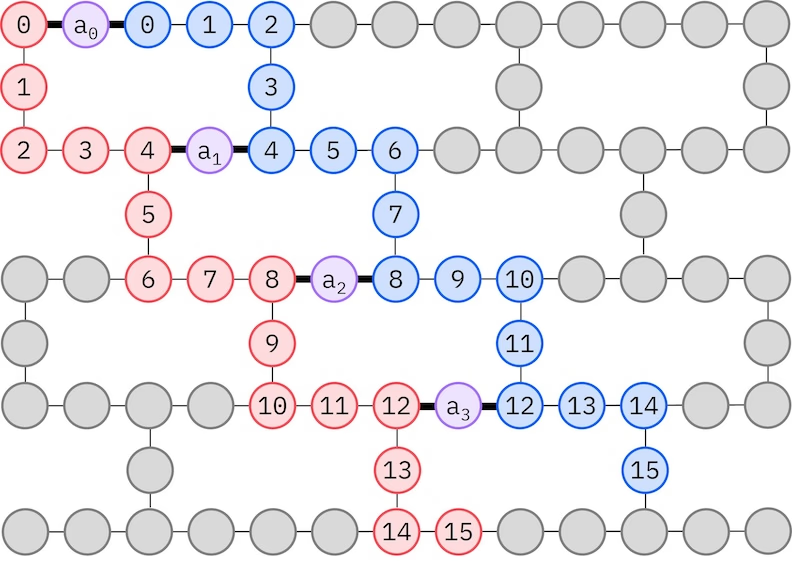
กล่าวอีกนัยหนึ่ง ถ้าเมทริกซ์ $\mathbf{J}$ มีค่าที่ไม่ใช่ศูนย์เฉพาะที่ index ที่ระบุในสามเหลี่ยมบน เทอม $e^{i \mathcal{J}_k}$ ก็สามารถใช้งานได้บน topology แบบ square โดยไม่ใช้ swap gate ใด ๆ ในความลึกคงที่ แน่นอนว่าการกำหนดข้อจำกัดดังกล่าวบน ansatz ทำให้มันมีความ expressive น้อยลง ดังนั้นอาจต้องการการทำซ้ำ ansatz มากขึ้น

ฮาร์ดแวร์ IBM® มี topology ของ Qubit แบบ heavy-hex lattice ซึ่งในกรณีนี้เราสามารถใช้รูปแบบ "zig-zag" ตามที่แสดงด้านล่าง ในรูปแบบนี้ orbital ที่มี spin เดียวกันจะถูก map ไปยัง Qubit ที่มี line topology (วงกลมสีแดงและสีน้ำเงิน) และการเชื่อมต่อระหว่าง orbital ที่มี spin ต่างกันมีอยู่ทุก spatial orbital ที่ 4 โดยการเชื่อมต่อจะถูกอำนวยความสะดวกโดย ancilla Qubit (วงกลมสีม่วง) ในกรณีนี้ ข้อจำกัด index คือ

$$\begin{align*} \mathbf{J}^{\alpha\alpha} &: \set{(p, p+1) \; , \; p = 0, \ldots, N-2} \\ \mathbf{J}^{\alpha\beta} &: \set{(p, p) \;, \; p = 0, 4, 8, \ldots (p \leq N-1)} \end{align*}$$

Self-consistent configuration recovery

กระบวนการ self-consistent configuration recovery ถูกออกแบบมาเพื่อดึงสัญญาณให้ได้มากที่สุดจากตัวอย่างควอนตัมที่มีสัญญาณรบกวน เนื่องจาก Hamiltonian ของโมเลกุลอนุรักษ์จำนวนอนุภาคและ spin Z จึงสมเหตุสมผลที่จะเลือก circuit ansatz ที่อนุรักษ์สมมาตรเหล่านี้ด้วย เมื่อนำไปใช้กับสถานะ Hartree-Fock สถานะที่ได้จะมีจำนวนอนุภาคและ spin Z คงที่ในการตั้งค่าที่ไม่มีสัญญาณรบกวน ดังนั้น ครึ่ง spin-$\alpha$ และ spin-$\beta$ ของ bitstring ใด ๆ ที่สุ่มจากสถานะนี้ควรมีHamming weight เดียวกับสถานะ Hartree-Fock เนื่องจากมีสัญญาณรบกวนในโปรเซสเซอร์ควอนตัมปัจจุบัน bitstring บางอันที่วัดได้จะละเมิดคุณสมบัตินี้ รูปแบบง่าย ๆ ของ postselection จะทิ้ง bitstring เหล่านี้ แต่นั่นสิ้นเปลือง เพราะ bitstring เหล่านั้นอาจยังมีสัญญาณอยู่บ้าง กระบวนการ self-consistent recovery พยายามกู้คืนสัญญาณบางส่วนนั้นใน post-processing กระบวนการนี้เป็นแบบวนซ้ำและต้องการเป็น input ค่าประมาณของค่าครอบครองเฉลี่ยของแต่ละ orbital ใน ground state ซึ่งคำนวณจากตัวอย่างดิบก่อน กระบวนการจะรันในลูป และแต่ละรอบมีขั้นตอนดังนี้:

1. สำหรับ bitstring แต่ละอันที่ละเมิดสมมาตรที่ระบุ ให้พลิก bit ด้วยกระบวนการแบบความน่าจะเป็นที่ออกแบบมาเพื่อให้ bitstring ใกล้เคียงกับค่าประมาณปัจจุบันของค่าครอบครอง orbital เฉลี่ยมากขึ้น เพื่อให้ได้ bitstring ใหม่
2. รวบรวม bitstring เก่าและใหม่ทั้งหมดที่ตอบสนองสมมาตร และสุ่มตัวอย่างย่อยของขนาดคงที่ที่กำหนดไว้ล่วงหน้า
3. สำหรับชุดย่อยของ bitstring แต่ละชุด ให้ project Hamiltonian ลงในซับสเปซที่ถูก span โดย basis vector ที่สอดคล้องกัน (ดูส่วนก่อนหน้า สำหรับคำอธิบายของ basis vector เหล่านี้) และคำนวณค่าประมาณ ground state ของ Hamiltonian ที่ถูก project บนคอมพิวเตอร์คลาสสิก
4. อัปเดตค่าประมาณของค่าครอบครอง orbital เฉลี่ยด้วยค่าประมาณ ground state ที่มีพลังงานต่ำที่สุด

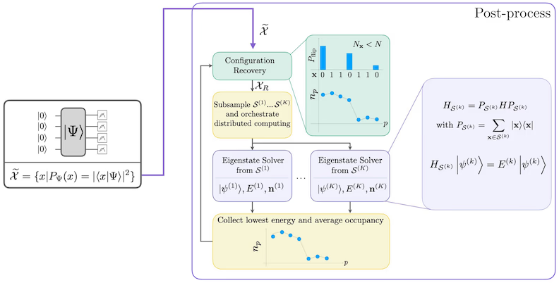
แผนภาพขั้นตอนการทำงาน SQD

ขั้นตอนการทำงาน SQD แสดงในแผนภาพต่อไปนี้:

ข้อกำหนด

ก่อนเริ่มบทแนะนำนี้ ให้แน่ใจว่าได้ติดตั้งสิ่งต่อไปนี้แล้ว:

• Qiskit SDK v1.0 หรือใหม่กว่า พร้อมรองรับการแสดงผล
• Qiskit Runtime v0.22 หรือใหม่กว่า (pip install qiskit-ibm-runtime)
• SQD Qiskit addon v0.11 หรือใหม่กว่า (pip install qiskit-addon-sqd)
• ffsim v0.0.58 หรือใหม่กว่า (pip install ffsim)

การตั้งค่า

# Added by doQumentation — required packages for this notebook
!pip install -q ffsim matplotlib numpy pyscf qiskit qiskit-addon-sqd qiskit-ibm-runtime rustworkx

import pyscf
import pyscf.cc
import pyscf.mcscf
import ffsim
import numpy as np
import matplotlib.pyplot as plt

from qiskit import QuantumCircuit, QuantumRegister
from qiskit.transpiler.preset_passmanagers import generate_preset_pass_manager

from qiskit_ibm_runtime import QiskitRuntimeService
from qiskit_ibm_runtime import SamplerV2 as Sampler

ขั้นตอนที่ 1: Map input คลาสสิกไปยังปัญหาควอนตัม

ในบทแนะนำนี้ เราจะหาค่าประมาณของ ground state ของโมเลกุลที่สมดุลใน cc-pVDZ basis set ก่อนอื่น เราระบุโมเลกุลและคุณสมบัติของมัน

# Specify molecule properties
open_shell = False
spin_sq = 0

# Build N2 molecule
mol = pyscf.gto.Mole()
mol.build(
    atom=[["N", (0, 0, 0)], ["N", (1.0, 0, 0)]],
    basis="cc-pvdz",
    symmetry="Dooh",
)

# Define active space
n_frozen = 2
active_space = range(n_frozen, mol.nao_nr())

# Get molecular integrals
scf = pyscf.scf.RHF(mol).run()
num_orbitals = len(active_space)
n_electrons = int(sum(scf.mo_occ[active_space]))
num_elec_a = (n_electrons + mol.spin) // 2
num_elec_b = (n_electrons - mol.spin) // 2
cas = pyscf.mcscf.CASCI(scf, num_orbitals, (num_elec_a, num_elec_b))
mo = cas.sort_mo(active_space, base=0)
hcore, nuclear_repulsion_energy = cas.get_h1cas(mo)
eri = pyscf.ao2mo.restore(1, cas.get_h2cas(mo), num_orbitals)

# Store reference energy from SCI calculation performed separately
exact_energy = -109.22690201485733

converged SCF energy = -108.929838385609

ก่อนสร้าง Circuit LUCJ ansatz เราทำการคำนวณ CCSD ในเซลล์โค้ดต่อไปนี้ก่อน amplitude $t_1$ และ $t_2$ จากการคำนวณนี้จะถูกใช้เพื่อ initialize พารามิเตอร์ของ ansatz

# Get CCSD t2 amplitudes for initializing the ansatz
ccsd = pyscf.cc.CCSD(
    scf, frozen=[i for i in range(mol.nao_nr()) if i not in active_space]
).run()
t1 = ccsd.t1
t2 = ccsd.t2

E(CCSD) = -109.2177884185543  E_corr = -0.2879500329450045

ตอนนี้ เราใช้ ffsim เพื่อสร้าง Circuit ansatz เนื่องจากโมเลกุลของเรามีสถานะ Hartree-Fock แบบ closed-shell เราจึงใช้ตัวแปรที่สมดุลด้าน spin ของ UCJ ansatz ได้แก่ UCJOpSpinBalanced เราส่งผ่าน interaction pair ที่เหมาะสมสำหรับ topology ของ Qubit แบบ heavy-hex lattice (ดูส่วนพื้นฐานเกี่ยวกับ LUCJ ansatz) เราตั้ง optimize=True ในเมธอด from_t_amplitudes เพื่อเปิดใช้การ double-factorization แบบ "compressed" ของ amplitude $t_2$ (ดู The local unitary cluster Jastrow (LUCJ) ansatz ในเอกสาร ffsim สำหรับรายละเอียด)

n_reps = 1
alpha_alpha_indices = [(p, p + 1) for p in range(num_orbitals - 1)]
alpha_beta_indices = [(p, p) for p in range(0, num_orbitals, 4)]

ucj_op = ffsim.UCJOpSpinBalanced.from_t_amplitudes(
    t2=t2,
    t1=t1,
    n_reps=n_reps,
    interaction_pairs=(alpha_alpha_indices, alpha_beta_indices),
    # Setting optimize=True enables the "compressed" factorization
    optimize=True,
    # Limit the number of optimization iterations to prevent the code cell from running
    # too long. Removing this line may improve results.
    options=dict(maxiter=1000),
)

nelec = (num_elec_a, num_elec_b)

# create an empty quantum circuit
qubits = QuantumRegister(2 * num_orbitals, name="q")
circuit = QuantumCircuit(qubits)

# prepare Hartree-Fock state as the reference state and append it to the quantum circuit
circuit.append(ffsim.qiskit.PrepareHartreeFockJW(num_orbitals, nelec), qubits)

# apply the UCJ operator to the reference state
circuit.append(ffsim.qiskit.UCJOpSpinBalancedJW(ucj_op), qubits)
circuit.measure_all()

ขั้นตอนที่ 2: ปรับแต่งปัญหาสำหรับการรันบนฮาร์ดแวร์ควอนตัม

ต่อไป เราปรับแต่ง Circuit สำหรับฮาร์ดแวร์เป้าหมาย

service = QiskitRuntimeService()
backend = service.least_busy(
    operational=True, simulator=False, min_num_qubits=133
)

print(f"Using backend {backend.name}")

Using backend ibm_fez

เราแนะนำขั้นตอนต่อไปนี้เพื่อปรับแต่ง ansatz และทำให้เข้ากันได้กับฮาร์ดแวร์

• เลือก physical Qubit (initial_layout) จากฮาร์ดแวร์เป้าหมายที่ยึดตามรูปแบบ "zig-zag" ที่อธิบายไว้ก่อนหน้า การจัด Qubit ในรูปแบบนี้นำไปสู่ Circuit ที่เข้ากันได้กับฮาร์ดแวร์อย่างมีประสิทธิภาพพร้อม Gate น้อยลง ที่นี่ เราใส่โค้ดบางส่วนเพื่อทำให้การเลือกรูปแบบ "zig-zag" เป็นอัตโนมัติโดยใช้ scoring heuristic เพื่อลดข้อผิดพลาดที่เกี่ยวข้องกับ layout ที่เลือก
• สร้าง staged pass manager โดยใช้ฟังก์ชัน generate_preset_pass_manager จาก Qiskit พร้อม backend และ initial_layout ที่เลือก
• ตั้ง stage pre_init ของ staged pass manager เป็น ffsim.qiskit.PRE_INIT ffsim.qiskit.PRE_INIT รวม Qiskit Transpiler pass ที่แยกย่อย Gate เป็น orbital rotation และ merge orbital rotation เพื่อให้มี Gate น้อยลงใน Circuit สุดท้าย
• รัน pass manager บน Circuit ของคุณ

โค้ดสำหรับการเลือก layout "zig-zag" โดยอัตโนมัติ

from typing import Sequence

import rustworkx
from qiskit.providers import BackendV2
from rustworkx import NoEdgeBetweenNodes, PyGraph

IBM_TWO_Q_GATES = {"cx", "ecr", "cz"}

def create_linear_chains(num_orbitals: int) -> PyGraph:
    """In zig-zag layout, there are two linear chains (with connecting qubits between
    the chains). This function creates those two linear chains: a rustworkx PyGraph
    with two disconnected linear chains. Each chain contains `num_orbitals` number
    of nodes, that is, in the final graph there are `2 * num_orbitals` number of nodes.

    Args:
        num_orbitals (int): Number orbitals or nodes in each linear chain. They are
            also known as alpha-alpha interaction qubits.

    Returns:
        A rustworkx.PyGraph with two disconnected linear chains each with `num_orbitals`
            number of nodes.
    """
    G = rustworkx.PyGraph()

    for n in range(num_orbitals):
        G.add_node(n)

    for n in range(num_orbitals - 1):
        G.add_edge(n, n + 1, None)

    for n in range(num_orbitals, 2 * num_orbitals):
        G.add_node(n)

    for n in range(num_orbitals, 2 * num_orbitals - 1):
        G.add_edge(n, n + 1, None)

    return G

def create_lucj_zigzag_layout(
    num_orbitals: int, backend_coupling_graph: PyGraph
) -> tuple[PyGraph, int]:
    """This function creates the complete zigzag graph that 'can be mapped' to an IBM QPU with
    heavy-hex connectivity (the zigzag must be an isomorphic sub-graph to the QPU/backend
    coupling graph for it to be mapped).
    The zigzag pattern includes both linear chains (alpha-alpha interactions) and connecting
    qubits between the linear chains (alpha-beta interactions).

    Args:
        num_orbitals (int): Number of orbitals, that is, number of nodes in each alpha-alpha linear chain.
        backend_coupling_graph (PyGraph): The coupling graph of the backend on which the LUCJ ansatz
            will be mapped and run. This function takes the coupling graph as a undirected
            `rustworkx.PyGraph` where there is only one 'undirected' edge between two nodes,
            that is, qubits. Usually, the coupling graph of a IBM backend is directed (for example, Eagle devices
            such as ibm_brisbane) or may have two edges between two nodes (for example, Heron `ibm_torino`).
            A user needs to be make such graphs undirected and/or remove duplicate edges to make them
            compatible with this function.

    Returns:
        G_new (PyGraph): The graph with IBM backend compliant zigzag pattern.
        num_alpha_beta_qubits (int): Number of connecting qubits between the linear chains
            in the zigzag pattern. While we want as many connecting (alpha-beta) qubits between
            the linear (alpha-alpha) chains, we cannot accommodate all due to qubit and connectivity
            constraints of backends. This is the maximum number of connecting qubits the zigzag pattern
            can have while being backend compliant (that is, isomorphic to backend coupling graph).
    """
    isomorphic = False
    G = create_linear_chains(num_orbitals=num_orbitals)

    num_iters = num_orbitals
    while not isomorphic:
        G_new = G.copy()
        num_alpha_beta_qubits = 0
        for n in range(num_iters):
            if n % 4 == 0:
                new_node = 2 * num_orbitals + num_alpha_beta_qubits
                G_new.add_node(new_node)
                G_new.add_edge(n, new_node, None)
                G_new.add_edge(new_node, n + num_orbitals, None)
                num_alpha_beta_qubits = num_alpha_beta_qubits + 1
        isomorphic = rustworkx.is_subgraph_isomorphic(
            backend_coupling_graph, G_new
        )
        num_iters -= 1

    return G_new, num_alpha_beta_qubits

def lightweight_layout_error_scoring(
    backend: BackendV2,
    virtual_edges: Sequence[Sequence[int]],
    physical_layouts: Sequence[int],
    two_q_gate_name: str,
) -> list[list[list[int], float]]:
    """Lightweight and heuristic function to score isomorphic layouts. There can be many zigzag patterns,
    each with different set of physical qubits, that can be mapped to a backend. Some of them may
    include less noise qubits and couplings than others. This function computes a simple error score
    for each such layout. It sums up 2Q gate error for all couplings in the zigzag pattern (layout) and
    measurement of errors of physical qubits in the layout to compute the error score.

    Note:
        This lightweight scoring can be refined using concepts such as mapomatic.

    Args:
        backend (BackendV2): A backend.
        virtual_edges (Sequence[Sequence[int]]): Edges in the device compliant zigzag pattern where
            nodes are numbered from 0 to (2 * num_orbitals + num_alpha_beta_qubits).
        physical_layouts (Sequence[int]): All physical layouts of the zigzag pattern that are isomorphic
            to each other and to the larger backend coupling map.
        two_q_gate_name (str): The name of the two-qubit gate of the backend. The name is used for fetching
            two-qubit gate error from backend properties.

    Returns:
        scores (list): A list of lists where each sublist contains two items. First item is the layout, and
            second item is a float representing error score of the layout. The layouts in the `scores` are
            sorted in the ascending order of error score.
    """
    props = backend.properties()
    scores = []
    for layout in physical_layouts:
        total_2q_error = 0
        for edge in virtual_edges:
            physical_edge = (layout[edge[0]], layout[edge[1]])
            try:
                ge = props.gate_error(two_q_gate_name, physical_edge)
            except Exception:
                ge = props.gate_error(two_q_gate_name, physical_edge[::-1])
            total_2q_error += ge
        total_measurement_error = 0
        for qubit in layout:
            meas_error = props.readout_error(qubit)
            total_measurement_error += meas_error
        scores.append([layout, total_2q_error + total_measurement_error])

    return sorted(scores, key=lambda x: x[1])

def _make_backend_cmap_pygraph(backend: BackendV2) -> PyGraph:
    graph = backend.coupling_map.graph
    if not graph.is_symmetric():
        graph.make_symmetric()
    backend_coupling_graph = graph.to_undirected()

    edge_list = backend_coupling_graph.edge_list()
    removed_edge = []
    for edge in edge_list:
        if set(edge) in removed_edge:
            continue
        try:
            backend_coupling_graph.remove_edge(edge[0], edge[1])
            removed_edge.append(set(edge))
        except NoEdgeBetweenNodes:
            pass

    return backend_coupling_graph

def get_zigzag_physical_layout(
    num_orbitals: int, backend: BackendV2, score_layouts: bool = True
) -> tuple[list[int], int]:
    """The main function that generates the zigzag pattern with physical qubits that can be used
    as an `intial_layout` in a preset passmanager/transpiler.

    Args:
        num_orbitals (int): Number of orbitals.
        backend (BackendV2): A backend.
        score_layouts (bool): Optional. If `True`, it uses the `lightweight_layout_error_scoring`
            function to score the isomorphic layouts and returns the layout with less erroneous qubits.
            If `False`, returns the first isomorphic subgraph.

    Returns:
        A tuple of device compliant layout (list[int]) with zigzag pattern and an int representing
            number of alpha-beta-interactions.
    """
    backend_coupling_graph = _make_backend_cmap_pygraph(backend=backend)

    G, num_alpha_beta_qubits = create_lucj_zigzag_layout(
        num_orbitals=num_orbitals,
        backend_coupling_graph=backend_coupling_graph,
    )

    isomorphic_mappings = rustworkx.vf2_mapping(
        backend_coupling_graph, G, subgraph=True
    )
    isomorphic_mappings = list(isomorphic_mappings)

    edges = list(G.edge_list())

    layouts = []
    for mapping in isomorphic_mappings:
        initial_layout = [None] * (2 * num_orbitals + num_alpha_beta_qubits)
        for key, value in mapping.items():
            initial_layout[value] = key
        layouts.append(initial_layout)

    two_q_gate_name = IBM_TWO_Q_GATES.intersection(
        backend.configuration().basis_gates
    ).pop()

    if score_layouts:
        scores = lightweight_layout_error_scoring(
            backend=backend,
            virtual_edges=edges,
            physical_layouts=layouts,
            two_q_gate_name=two_q_gate_name,
        )

        return scores[0][0][:-num_alpha_beta_qubits], num_alpha_beta_qubits

    return layouts[0][:-num_alpha_beta_qubits], num_alpha_beta_qubits

initial_layout, _ = get_zigzag_physical_layout(num_orbitals, backend=backend)

pass_manager = generate_preset_pass_manager(
    optimization_level=3, backend=backend, initial_layout=initial_layout
)

# without PRE_INIT passes
isa_circuit = pass_manager.run(circuit)
print(f"Gate counts (w/o pre-init passes): {isa_circuit.count_ops()}")

# with PRE_INIT passes
# We will use the circuit generated by this pass manager for hardware execution
pass_manager.pre_init = ffsim.qiskit.PRE_INIT
isa_circuit = pass_manager.run(circuit)
print(f"Gate counts (w/ pre-init passes): {isa_circuit.count_ops()}")

Gate counts (w/o pre-init passes): OrderedDict({'rz': 12438, 'sx': 12169, 'cz': 3986, 'x': 573, 'measure': 52, 'barrier': 1})
Gate counts (w/ pre-init passes): OrderedDict({'sx': 7059, 'rz': 6962, 'cz': 1876, 'measure': 52, 'x': 35, 'barrier': 1})

ขั้นตอนที่ 3: รันด้วย Qiskit primitives

หลังจากปรับแต่ง Circuit ให้พร้อมสำหรับการรันบนฮาร์ดแวร์แล้ว เราก็พร้อมรันบนฮาร์ดแวร์จริงและเก็บตัวอย่างสำหรับการประมาณพลังงาน ground state เนื่องจากมีเพียง Circuit เดียว เราจะใช้ Job execution mode ของ Qiskit Runtime เพื่อรัน Circuit

sampler = Sampler(mode=backend)
job = sampler.run([isa_circuit], shots=100_000)

primitive_result = job.result()
pub_result = primitive_result[0]

ขั้นตอนที่ 4: ประมวลผลและแสดงผลลัพธ์ในรูปแบบคลาสสิก

ตอนนี้เราจะประมาณพลังงาน ground state ของ Hamiltonian โดยใช้ฟังก์ชัน diagonalize_fermionic_hamiltonian ฟังก์ชันนี้ทำกระบวนการ self-consistent configuration recovery เพื่อปรับปรุงตัวอย่างควอนตัมที่มีสัญญาณรบกวนแบบวนซ้ำ เพื่อให้การประมาณพลังงานดีขึ้น เราส่ง callback function เข้าไปเพื่อบันทึกผลลัพธ์ระหว่างกลางสำหรับการวิเคราะห์ในภายหลัง ดู API documentation สำหรับคำอธิบาย argument ของ diagonalize_fermionic_hamiltonian

from functools import partial

from qiskit_addon_sqd.fermion import (
    SCIResult,
    diagonalize_fermionic_hamiltonian,
    solve_sci_batch,
)

# SQD options
energy_tol = 1e-3
occupancies_tol = 1e-3
max_iterations = 5

# Eigenstate solver options
num_batches = 3
samples_per_batch = 300
symmetrize_spin = True
carryover_threshold = 1e-4
max_cycle = 200

# Pass options to the built-in eigensolver. If you just want to use the defaults,
# you can omit this step, in which case you would not specify the sci_solver argument
# in the call to diagonalize_fermionic_hamiltonian below.
sci_solver = partial(solve_sci_batch, spin_sq=0.0, max_cycle=max_cycle)

# List to capture intermediate results
result_history = []

def callback(results: list[SCIResult]):
    result_history.append(results)
    iteration = len(result_history)
    print(f"Iteration {iteration}")
    for i, result in enumerate(results):
        print(f"\tSubsample {i}")
        print(f"\t\tEnergy: {result.energy + nuclear_repulsion_energy}")
        print(
            f"\t\tSubspace dimension: {np.prod(result.sci_state.amplitudes.shape)}"
        )

result = diagonalize_fermionic_hamiltonian(
    hcore,
    eri,
    pub_result.data.meas,
    samples_per_batch=samples_per_batch,
    norb=num_orbitals,
    nelec=nelec,
    num_batches=num_batches,
    energy_tol=energy_tol,
    occupancies_tol=occupancies_tol,
    max_iterations=max_iterations,
    sci_solver=sci_solver,
    symmetrize_spin=symmetrize_spin,
    carryover_threshold=carryover_threshold,
    callback=callback,
    seed=12345,
)

Iteration 1
	Subsample 0
		Energy: -108.97781410104506
		Subspace dimension: 28561
	Subsample 1
		Energy: -108.97781410104506
		Subspace dimension: 28561
	Subsample 2
		Energy: -108.97781410104506
		Subspace dimension: 28561
Iteration 2
	Subsample 0
		Energy: -109.05150860754739
		Subspace dimension: 287296
	Subsample 1
		Energy: -109.08152283263908
		Subspace dimension: 264196
	Subsample 2
		Energy: -109.11636893067873
		Subspace dimension: 284089
Iteration 3
	Subsample 0
		Energy: -109.15878555367885
		Subspace dimension: 429025
	Subsample 1
		Energy: -109.16462831275786
		Subspace dimension: 473344
	Subsample 2
		Energy: -109.15895026995382
		Subspace dimension: 435600
Iteration 4
	Subsample 0
		Energy: -109.17784051223317
		Subspace dimension: 622521
	Subsample 1
		Energy: -109.1774651326829
		Subspace dimension: 657721
	Subsample 2
		Energy: -109.18085212360191
		Subspace dimension: 617796
Iteration 5
	Subsample 0
		Energy: -109.18636242518915
		Subspace dimension: 815409
	Subsample 1
		Energy: -109.18451014767518
		Subspace dimension: 837225
	Subsample 2
		Energy: -109.18333728638888
		Subspace dimension: 857476

แสดงผลลัพธ์

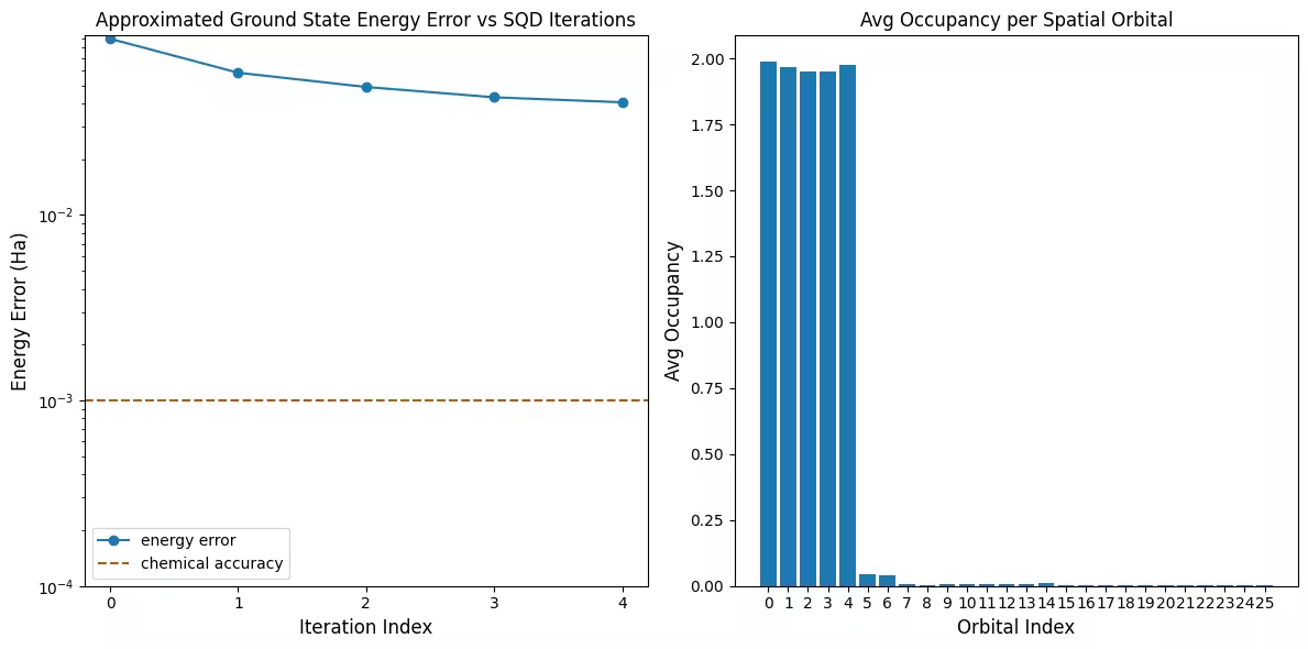
กราฟแรกแสดงให้เห็นว่าหลังจากวนซ้ำไปสองสามรอบ เราสามารถประมาณพลังงาน ground state ได้ภายในระยะ ~41 mH (ความแม่นยำทางเคมีโดยทั่วไปยอมรับที่ 1 kcal/mol $\approx$ 1.6 mH) พลังงานสามารถปรับปรุงให้ดีขึ้นได้โดยการเพิ่มจำนวนรอบของ configuration recovery หรือเพิ่มจำนวนตัวอย่างต่อ batch

กราฟที่สองแสดงค่าการครอบครองเฉลี่ยของแต่ละ spatial orbital หลังจากการวนซ้ำครั้งสุดท้าย จะเห็นได้ว่าทั้งอิเล็กตรอน spin-up และ spin-down ครอบครอง 5 orbital แรกด้วยความน่าจะเป็นสูงในคำตอบของเรา

# Data for energies plot
x1 = range(len(result_history))
min_e = [
    min(result, key=lambda res: res.energy).energy + nuclear_repulsion_energy
    for result in result_history
]
e_diff = [abs(e - exact_energy) for e in min_e]
yt1 = [1.0, 1e-1, 1e-2, 1e-3, 1e-4]

# Chemical accuracy (+/- 1 milli-Hartree)
chem_accuracy = 0.001

# Data for avg spatial orbital occupancy
y2 = np.sum(result.orbital_occupancies, axis=0)
x2 = range(len(y2))

fig, axs = plt.subplots(1, 2, figsize=(12, 6))

# Plot energies
axs[0].plot(x1, e_diff, label="energy error", marker="o")
axs[0].set_xticks(x1)
axs[0].set_xticklabels(x1)
axs[0].set_yticks(yt1)
axs[0].set_yticklabels(yt1)
axs[0].set_yscale("log")
axs[0].set_ylim(1e-4)
axs[0].axhline(
    y=chem_accuracy,
    color="#BF5700",
    linestyle="--",
    label="chemical accuracy",
)
axs[0].set_title("Approximated Ground State Energy Error vs SQD Iterations")
axs[0].set_xlabel("Iteration Index", fontdict={"fontsize": 12})
axs[0].set_ylabel("Energy Error (Ha)", fontdict={"fontsize": 12})
axs[0].legend()

# Plot orbital occupancy
axs[1].bar(x2, y2, width=0.8)
axs[1].set_xticks(x2)
axs[1].set_xticklabels(x2)
axs[1].set_title("Avg Occupancy per Spatial Orbital")
axs[1].set_xlabel("Orbital Index", fontdict={"fontsize": 12})
axs[1].set_ylabel("Avg Occupancy", fontdict={"fontsize": 12})

plt.tight_layout()
plt.show()

แบบสำรวจ Tutorial

Link to survey

Note: This survey is provided by IBM Quantum and relates to the original English content. To give feedback on doQumentation's website, translations, or code execution, please open a GitHub issue.

กรุณาทำแบบสำรวจสั้น ๆ นี้เพื่อให้ข้อเสนอแนะเกี่ยวกับ tutorial นี้ ความคิดเห็นของคุณจะช่วยให้เราปรับปรุงเนื้อหาและประสบการณ์การใช้งาน