การวิเคราะห์เมทริกซ์เชิงควอนตัมแบบ Krylov โดยใช้การสุ่มตัวอย่างสำหรับโมเดลแลตทิซเฟอร์มิออน

ประมาณการการใช้งาน: เก้าวินาทีบนโปรเซสเซอร์ Heron r2 (หมายเหตุ: นี่เป็นเพียงการประมาณการเท่านั้น เวลาจริงของคุณอาจแตกต่างออกไป)

พื้นหลัง

บทแนะนำนี้แสดงวิธีใช้ sample-based quantum diagonalization (SQD) เพื่อประมาณพลังงานสถานะพื้นฐานของโมเดลแลตทิซเฟอร์มิออน โดยเฉพาะอย่างยิ่ง เราศึกษา one-dimensional single-impurity Anderson model (SIAM) ซึ่งใช้อธิบายสิ่งเจือปนแม่เหล็กที่ฝังอยู่ในโลหะ

บทแนะนำนี้ทำตามขั้นตอนการทำงานที่คล้ายกับบทแนะนำที่เกี่ยวข้อง Sample-based quantum diagonalization of a chemistry Hamiltonian แต่ความแตกต่างหลักอยู่ที่วิธีการสร้าง Circuit ควอนตัม บทแนะนำอื่นใช้ heuristic variational ansatz ซึ่งน่าสนใจสำหรับ Hamiltonian ทางเคมีที่อาจมีพจน์ปฏิสัมพันธ์หลายล้านพจน์ ในทางกลับกัน บทแนะนำนี้ใช้ Circuit ที่ประมาณการวิวัฒนาการตามเวลาด้วย Hamiltonian Circuit เหล่านี้อาจมีความลึกมาก ซึ่งทำให้วิธีนี้เหมาะสมกว่าสำหรับการประยุกต์ใช้กับโมเดลแลตทิซ เวกเตอร์สถานะที่ Circuit เหล่านี้สร้างขึ้นก่อให้เกิดฐานสำหรับ Krylov subspace และด้วยเหตุนี้ อัลกอริทึมจึงสามารถพิสูจน์ได้และลู่เข้าสู่สถานะพื้นฐานอย่างมีประสิทธิภาพ ภายใต้ข้อสมมติฐานที่เหมาะสม

วิธีการที่ใช้ในบทแนะนำนี้สามารถมองได้ว่าเป็นการผสมผสานเทคนิคที่ใช้ใน SQD และ Krylov quantum diagonalization (KQD) วิธีการรวมนี้บางครั้งเรียกว่า sample-based Krylov quantum diagonalization (SQKD) ดู Krylov quantum diagonalization of lattice Hamiltonians สำหรับบทแนะนำเกี่ยวกับวิธี KQD

บทแนะนำนี้อ้างอิงจากงานวิจัย "Quantum-Centric Algorithm for Sample-Based Krylov Diagonalization" ซึ่งสามารถอ้างถึงเพื่อดูรายละเอียดเพิ่มเติมได้

Single-impurity Anderson model (SIAM)

SIAM Hamiltonian หนึ่งมิติเป็นผลรวมของสามพจน์:

$$H = H_{\textrm{imp}}+ H_\textrm{bath} + H_\textrm{hyb},$$

โดยที่

$$\begin{align*} H_\textrm{imp} &= \varepsilon \left( \hat{n}_{d\uparrow} + \hat{n}_{d\downarrow} \right) + U \hat{n}_{d\uparrow}\hat{n}_{d\downarrow}, \\ H_\textrm{bath} &= -t \sum_{\substack{\mathbf{j} = 0\\ \sigma\in \{\uparrow, \downarrow\}}}^{L-1} \left(\hat{c}^\dagger_{\mathbf{j}, \sigma}\hat{c}_{\mathbf{j}+1, \sigma} + \hat{c}^\dagger_{\mathbf{j}+1, \sigma}\hat{c}_{\mathbf{j}, \sigma} \right), \\ H_\textrm{hyb} &= V\sum_{\sigma \in \{\uparrow, \downarrow \}} \left(\hat{d}^\dagger_\sigma \hat{c}_{0, \sigma} + \hat{c}^\dagger_{0, \sigma} \hat{d}_{\sigma} \right). \end{align*}$$

ที่นี่ $c^\dagger_{\mathbf{j},\sigma}/c_{\mathbf{j},\sigma}$ คือตัวดำเนินการสร้าง/ทำลายเฟอร์มิออนสำหรับตำแหน่ง bath ที่ $\mathbf{j}^{\textrm{th}}$ ที่มีสปิน $\sigma$, $\hat{d}^\dagger_{\sigma}/\hat{d}_{\sigma}$ คือตัวดำเนินการสร้าง/ทำลายสำหรับโหมดสิ่งเจือปน และ $\hat{n}_{d\sigma} = \hat{d}^\dagger_{\sigma} \hat{d}_{\sigma}$ ส่วน $t$, $U$ และ $V$ เป็นจำนวนจริงที่อธิบายปฏิสัมพันธ์การกระโดด on-site และ hybridization และ $\varepsilon$ เป็นจำนวนจริงที่ระบุศักย์เคมี

โปรดสังเกตว่า Hamiltonian นี้เป็นกรณีเฉพาะของ Hamiltonian อิเล็กตรอนปฏิสัมพันธ์ทั่วไป

$$\begin{align*} H &= \sum_{\substack{p, q \\ \sigma}} h_{pq} \hat{a}^\dagger_{p\sigma} \hat{a}_{q\sigma} + \sum_{\substack{p, q, r, s \\ \sigma \tau}} \frac{h_{pqrs}}{2} \hat{a}^\dagger_{p\sigma} \hat{a}^\dagger_{q\tau} \hat{a}_{s\tau} \hat{a}_{r\sigma} \\ &= H_1 + H_2, \end{align*}$$

โดยที่ $H_1$ ประกอบด้วยพจน์หนึ่งอนุภาค ซึ่งเป็นกำลังสองในตัวดำเนินการสร้างและทำลายเฟอร์มิออน และ $H_2$ ประกอบด้วยพจน์สองอนุภาค ซึ่งเป็นกำลังสี่ สำหรับ SIAM:

$$H_2 = U \hat{n}_{d\uparrow}\hat{n}_{d\downarrow}$$

และ $H_1$ มีพจน์ที่เหลือใน Hamiltonian เพื่อแทน Hamiltonian ด้วยโปรแกรม เราเก็บเมทริกซ์ $h_{pq}$ และเทนเซอร์ $h_{pqrs}$

ฐานตำแหน่งและฐานโมเมนตัม

เนื่องจากความสมมาตรการเลื่อนตำแหน่งโดยประมาณใน $H_\textrm{bath}$ เราจึงไม่คาดว่าสถานะพื้นฐานจะกระจายตัวน้อยในฐานตำแหน่ง (ฐานออร์บิทัลที่ระบุ Hamiltonian ข้างต้น) ประสิทธิภาพของ SQD รับประกันได้เฉพาะเมื่อสถานะพื้นฐานกระจายตัวน้อย นั่นคือมีน้ำหนักสำคัญบนสถานะฐานการคำนวณเพียงไม่กี่สถานะ เพื่อปรับปรุงความกระจัดกระจายของสถานะพื้นฐาน เราทำการจำลองในฐานออร์บิทัลที่ $H_\textrm{bath}$ เป็นแนวทแยง เราเรียกฐานนี้ว่า ฐานโมเมนตัม เนื่องจาก $H_\textrm{bath}$ เป็น Hamiltonian เฟอร์มิออนกำลังสอง จึงสามารถทำให้เป็นแนวทแยงได้อย่างมีประสิทธิภาพโดยการหมุนออร์บิทัล

การประมาณวิวัฒนาการตามเวลาด้วย Hamiltonian

เพื่อประมาณวิวัฒนาการตามเวลาด้วย Hamiltonian เราใช้การแตกตัวแบบ second order Trotter-Suzuki:

$$e^{-i \Delta t H} \approx e^{-i\frac{\Delta t}{2} H_2} e^{-i\Delta t H_1} e^{-i\frac{\Delta t}{2} H_2}.$$

ภายใต้ Jordan-Wigner transformation วิวัฒนาการตามเวลาด้วย $H_2$ เท่ากับ Gate CPhase เดียวระหว่างออร์บิทัล spin-up และ spin-down ที่ตำแหน่งสิ่งเจือปน เนื่องจาก $H_1$ เป็น Hamiltonian เฟอร์มิออนกำลังสอง วิวัฒนาการตามเวลาด้วย $H_1$ จึงเท่ากับการหมุนออร์บิทัล

สถานะฐาน Krylov $\{ |\psi_k\rangle \}_{k=0}^{D-1}$ โดยที่ $D$ คือมิติของ Krylov subspace ถูกสร้างขึ้นโดยการใช้ขั้นตอน Trotter ซ้ำ ดังนั้น

$$|\psi_k\rangle \approx \left[e^{-i\frac{\Delta t}{2} H_2} e^{-i\Delta t H_1} e^{-i\frac{\Delta t}{2} H_2} \right]^k\ket{\psi_0}.$$

ในขั้นตอนการทำงานแบบ SQD ต่อไปนี้ เราจะสุ่มตัวอย่างจากชุด Circuit นี้และประมวลผลชุด bitstring รวมกันด้วย SQD วิธีนี้แตกต่างจากที่ใช้ในบทแนะนำที่เกี่ยวข้อง Sample-based quantum diagonalization of a chemistry Hamiltonian ซึ่งสุ่มตัวอย่างจาก Circuit variational เชิงฮิวริสติกเดียว

ข้อกำหนด

ก่อนเริ่มบทแนะนำนี้ ตรวจสอบให้แน่ใจว่าติดตั้งสิ่งต่อไปนี้แล้ว:

• Qiskit SDK v1.0 หรือใหม่กว่า พร้อมรองรับ visualization
• Qiskit Runtime v0.22 หรือใหม่กว่า (pip install qiskit-ibm-runtime)
• SQD Qiskit addon v0.11 หรือใหม่กว่า (pip install qiskit-addon-sqd)
• ffsim (pip install ffsim)

ขั้นตอนที่ 1: แมปปัญหากับ Circuit ควอนตัม

ก่อนอื่น เราสร้าง SIAM Hamiltonian ในฐานตำแหน่ง โดย Hamiltonian แทนด้วยเมทริกซ์ $h_{pq}$ และเทนเซอร์ $h_{pqrs}$ จากนั้นเราหมุนไปยังฐานโมเมนตัม ในฐานตำแหน่ง เราวางสิ่งเจือปนไว้ที่ตำแหน่งแรก แต่เมื่อหมุนไปยังฐานโมเมนตัม เราย้ายสิ่งเจือปนไปยังตำแหน่งกลางเพื่อให้ปฏิสัมพันธ์กับออร์บิทัลอื่นได้ง่ายขึ้น

# Added by doQumentation — required packages for this notebook
!pip install -q ffsim matplotlib numpy qiskit qiskit-addon-sqd qiskit-ibm-runtime scipy

import numpy as np

def siam_hamiltonian(
    norb: int,
    hopping: float,
    onsite: float,
    hybridization: float,
    chemical_potential: float,
) -> tuple[np.ndarray, np.ndarray]:
    """Hamiltonian for the single-impurity Anderson model."""
    # Place the impurity on the first site
    impurity_orb = 0

    # One body matrix elements in the "position" basis
    h1e = np.zeros((norb, norb))
    np.fill_diagonal(h1e[:, 1:], -hopping)
    np.fill_diagonal(h1e[1:, :], -hopping)
    h1e[impurity_orb, impurity_orb + 1] = -hybridization
    h1e[impurity_orb + 1, impurity_orb] = -hybridization
    h1e[impurity_orb, impurity_orb] = chemical_potential

    # Two body matrix elements in the "position" basis
    h2e = np.zeros((norb, norb, norb, norb))
    h2e[impurity_orb, impurity_orb, impurity_orb, impurity_orb] = onsite

    return h1e, h2e

def momentum_basis(norb: int) -> np.ndarray:
    """Get the orbital rotation to change from the position to the momentum basis."""
    n_bath = norb - 1

    # Orbital rotation that diagonalizes the bath (non-interacting system)
    hopping_matrix = np.zeros((n_bath, n_bath))
    np.fill_diagonal(hopping_matrix[:, 1:], -1)
    np.fill_diagonal(hopping_matrix[1:, :], -1)
    _, vecs = np.linalg.eigh(hopping_matrix)

    # Expand to include impurity
    orbital_rotation = np.zeros((norb, norb))
    # Impurity is on the first site
    orbital_rotation[0, 0] = 1
    orbital_rotation[1:, 1:] = vecs

    # Move the impurity to the center
    new_index = n_bath // 2
    perm = np.r_[1 : (new_index + 1), 0, (new_index + 1) : norb]
    orbital_rotation = orbital_rotation[:, perm]

    return orbital_rotation

def rotated(
    h1e: np.ndarray, h2e: np.ndarray, orbital_rotation: np.ndarray
) -> tuple[np.ndarray, np.ndarray]:
    """Rotate the orbital basis of a Hamiltonian."""
    h1e_rotated = np.einsum(
        "ab,Aa,Bb->AB",
        h1e,
        orbital_rotation,
        orbital_rotation.conj(),
        optimize="greedy",
    )
    h2e_rotated = np.einsum(
        "abcd,Aa,Bb,Cc,Dd->ABCD",
        h2e,
        orbital_rotation,
        orbital_rotation.conj(),
        orbital_rotation,
        orbital_rotation.conj(),
        optimize="greedy",
    )
    return h1e_rotated, h2e_rotated

# Total number of spatial orbitals, including the bath sites and the impurity
# This should be an even number
norb = 20

# System is half-filled
nelec = (norb // 2, norb // 2)
# One orbital is the impurity, the rest are bath sites
n_bath = norb - 1

# Hamiltonian parameters
hybridization = 1.0
hopping = 1.0
onsite = 10.0
chemical_potential = -0.5 * onsite

# Generate Hamiltonian in position basis
h1e, h2e = siam_hamiltonian(
    norb=norb,
    hopping=hopping,
    onsite=onsite,
    hybridization=hybridization,
    chemical_potential=chemical_potential,
)

# Rotate to momentum basis
orbital_rotation = momentum_basis(norb)
h1e_momentum, h2e_momentum = rotated(h1e, h2e, orbital_rotation.T.conj())
# In the momentum basis, the impurity is placed in the center
impurity_index = n_bath // 2

ต่อไป เราสร้าง Circuit เพื่อสร้างสถานะฐาน Krylov สำหรับแต่ละชนิดสปิน สถานะเริ่มต้น $\ket{\psi_0}$ ถูกกำหนดโดยการซ้อนทับของการกระตุ้นทั้งหมดที่เป็นไปได้ของอิเล็กตรอนสามตัวที่ใกล้กับระดับ Fermi มากที่สุดไปยังโหมดว่างที่ใกล้ที่สุด 4 โหมด โดยเริ่มจากสถานะ $|00\cdots 0011 \cdots 11\rangle$ และทำได้โดยการใช้ XXPlusYYGate เจ็ดตัว สถานะที่วิวัฒนาการตามเวลาถูกสร้างขึ้นโดยการใช้ขั้นตอน Trotter อันดับสองซ้ำ

สำหรับคำอธิบายโดยละเอียดเพิ่มเติมเกี่ยวกับโมเดลนี้และวิธีการออกแบบ Circuit โปรดดู "Quantum-Centric Algorithm for Sample-Based Krylov Diagonalization"

from typing import Sequence

import ffsim
import scipy
from qiskit import QuantumCircuit, QuantumRegister
from qiskit.circuit import CircuitInstruction, Qubit
from qiskit.circuit.library import CPhaseGate, XGate, XXPlusYYGate

def prepare_initial_state(qubits: Sequence[Qubit], norb: int, nocc: int):
    """Prepare initial state."""
    x_gate = XGate()
    rot = XXPlusYYGate(0.5 * np.pi, -0.5 * np.pi)
    for i in range(nocc):
        yield CircuitInstruction(x_gate, [qubits[i]])
        yield CircuitInstruction(x_gate, [qubits[norb + i]])
    for i in range(3):
        for j in range(nocc - i - 1, nocc + i, 2):
            yield CircuitInstruction(rot, [qubits[j], qubits[j + 1]])
            yield CircuitInstruction(
                rot, [qubits[norb + j], qubits[norb + j + 1]]
            )
    yield CircuitInstruction(rot, [qubits[j + 1], qubits[j + 2]])
    yield CircuitInstruction(
        rot, [qubits[norb + j + 1], qubits[norb + j + 2]]
    )

def trotter_step(
    qubits: Sequence[Qubit],
    time_step: float,
    one_body_evolution: np.ndarray,
    h2e: np.ndarray,
    impurity_index: int,
    norb: int,
):
    """A Trotter step."""
    # Assume the two-body interaction is just the on-site interaction of the impurity
    onsite = h2e[
        impurity_index, impurity_index, impurity_index, impurity_index
    ]
    # Two-body evolution for half the time
    yield CircuitInstruction(
        CPhaseGate(-0.5 * time_step * onsite),
        [qubits[impurity_index], qubits[norb + impurity_index]],
    )
    # One-body evolution for the full time
    yield CircuitInstruction(
        ffsim.qiskit.OrbitalRotationJW(norb, one_body_evolution), qubits
    )
    # Two-body evolution for half the time
    yield CircuitInstruction(
        CPhaseGate(-0.5 * time_step * onsite),
        [qubits[impurity_index], qubits[norb + impurity_index]],
    )

# Time step
time_step = 0.2
# Number of Krylov basis states
krylov_dim = 8

# Initialize circuit
qubits = QuantumRegister(2 * norb, name="q")
circuit = QuantumCircuit(qubits)

# Generate initial state
for instruction in prepare_initial_state(qubits, norb=norb, nocc=norb // 2):
    circuit.append(instruction)
circuit.measure_all()

# Create list of circuits, starting with the initial state circuit
circuits = [circuit.copy()]

# Add time evolution circuits to the list
one_body_evolution = scipy.linalg.expm(-1j * time_step * h1e_momentum)
for i in range(krylov_dim - 1):
    # Remove measurements
    circuit.remove_final_measurements()
    # Append another Trotter step
    for instruction in trotter_step(
        qubits,
        time_step,
        one_body_evolution,
        h2e_momentum,
        impurity_index,
        norb,
    ):
        circuit.append(instruction)
    # Measure qubits
    circuit.measure_all()
    # Add a copy of the circuit to the list
    circuits.append(circuit.copy())

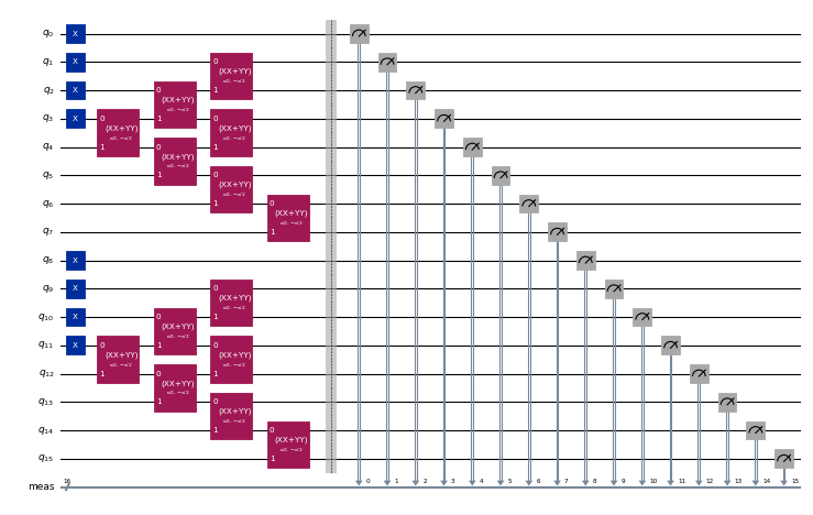
circuits[0].draw("mpl", scale=0.4, fold=-1)

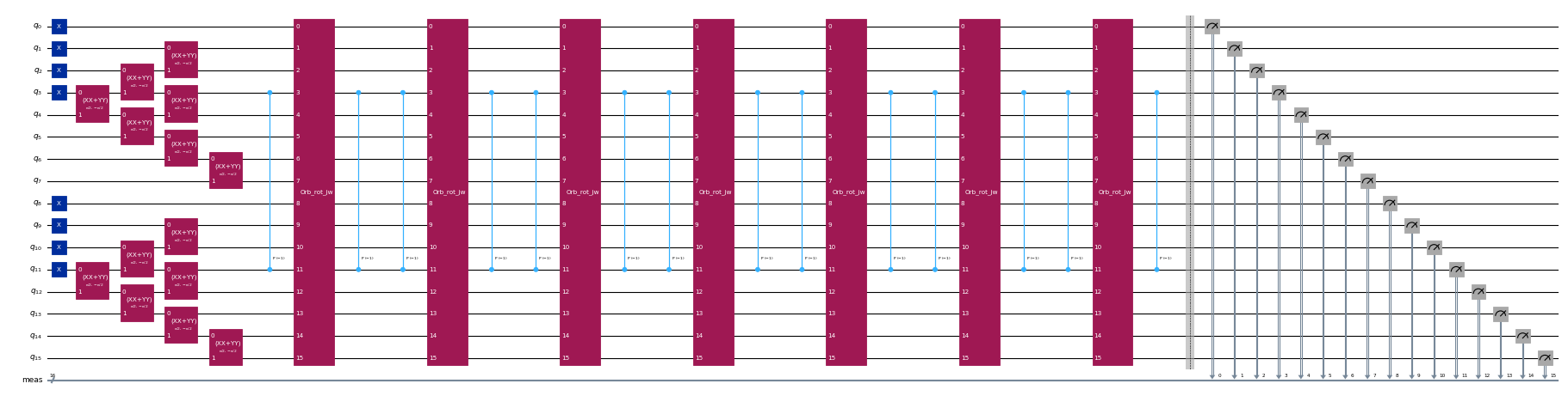
circuits[-1].draw("mpl", scale=0.4, fold=-1)

ขั้นตอนที่ 2: ปรับแต่งปัญหาสำหรับการรันแบบควอนตัม

เมื่อสร้าง Circuit แล้ว เราสามารถ optimize สำหรับ hardware เป้าหมายได้ เราเลือก QPU ที่ว่างที่สุดที่มีอย่างน้อย 127 Qubit ดูข้อมูลเพิ่มเติมที่ เอกสาร Qiskit IBM® Runtime

from qiskit_ibm_runtime import QiskitRuntimeService

service = QiskitRuntimeService()
backend = service.least_busy(
    operational=True, simulator=False, min_num_qubits=127
)
print(f"Using backend {backend.name}")

Using backend ibm_fez

ตอนนี้เราใช้ Qiskit เพื่อ transpile Circuit สำหรับ backend เป้าหมาย

from qiskit.transpiler import generate_preset_pass_manager

pass_manager = generate_preset_pass_manager(
    optimization_level=3, backend=backend
)
isa_circuits = pass_manager.run(circuits)

ขั้นตอนที่ 3: รันด้วย Qiskit primitives

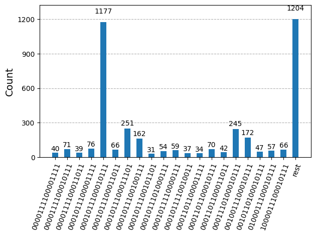
หลังจาก optimize วงจรสำหรับการรันบน hardware แล้ว เราก็พร้อมรันบน hardware จริงและเก็บตัวอย่างสำหรับการประมาณ ground state energy แล้ว หลังจากใช้ Sampler primitive เพื่อ sample bitstring จากแต่ละวงจร เราจะรวมผลลัพธ์ทั้งหมดเข้าด้วยกันเป็น counts dictionary เดียว และ plot 20 bitstring ที่ถูก sample บ่อยที่สุด

from qiskit.visualization import plot_histogram
from qiskit_ibm_runtime import SamplerV2 as Sampler

# Sample from the circuits
sampler = Sampler(backend)
job = sampler.run(isa_circuits, shots=500)

from qiskit.primitives import BitArray

# Combine the counts from the individual Trotter circuits
bit_array = BitArray.concatenate_shots(
    [result.data.meas for result in job.result()]
)

plot_histogram(bit_array.get_counts(), number_to_keep=20)

ขั้นตอนที่ 4: Post-process และคืนผลลัพธ์เป็น format ที่ต้องการ

ตอนนี้เราจะรัน SQD algorithm โดยใช้ฟังก์ชัน diagonalize_fermionic_hamiltonian ดู API documentation สำหรับคำอธิบาย argument ของฟังก์ชันนี้

from qiskit_addon_sqd.fermion import (
    SCIResult,
    diagonalize_fermionic_hamiltonian,
)

# List to capture intermediate results
result_history = []

def callback(results: list[SCIResult]):
    result_history.append(results)
    iteration = len(result_history)
    print(f"Iteration {iteration}")
    for i, result in enumerate(results):
        print(f"\tSubsample {i}")
        print(f"\t\tEnergy: {result.energy}")
        print(
            f"\t\tSubspace dimension: {np.prod(result.sci_state.amplitudes.shape)}"
        )

rng = np.random.default_rng(24)
result = diagonalize_fermionic_hamiltonian(
    h1e_momentum,
    h2e_momentum,
    bit_array,
    samples_per_batch=100,
    norb=norb,
    nelec=nelec,
    num_batches=3,
    max_iterations=5,
    symmetrize_spin=True,
    callback=callback,
    seed=rng,
)

Iteration 1
	Subsample 0
		Energy: -28.61321893815165
		Subspace dimension: 10609
	Subsample 1
		Energy: -28.628985564542244
		Subspace dimension: 13924
	Subsample 2
		Energy: -28.620151775558114
		Subspace dimension: 10404
Iteration 2
	Subsample 0
		Energy: -28.656893066053115
		Subspace dimension: 34225
	Subsample 1
		Energy: -28.65277622004119
		Subspace dimension: 38416
	Subsample 2
		Energy: -28.670856034959165
		Subspace dimension: 39601
Iteration 3
	Subsample 0
		Energy: -28.684787675404362
		Subspace dimension: 42436
	Subsample 1
		Energy: -28.676984757118426
		Subspace dimension: 50176
	Subsample 2
		Energy: -28.671581704249885
		Subspace dimension: 40804
Iteration 4
	Subsample 0
		Energy: -28.6859683054753
		Subspace dimension: 47961
	Subsample 1
		Energy: -28.69418206537316
		Subspace dimension: 51529
	Subsample 2
		Energy: -28.686083516445752
		Subspace dimension: 51529
Iteration 5
	Subsample 0
		Energy: -28.694665630711178
		Subspace dimension: 50625
	Subsample 1
		Energy: -28.69505984237118
		Subspace dimension: 47524
	Subsample 2
		Energy: -28.6942873883992
		Subspace dimension: 48841

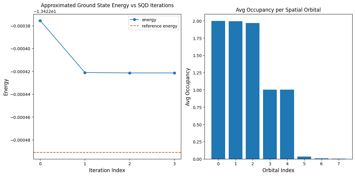
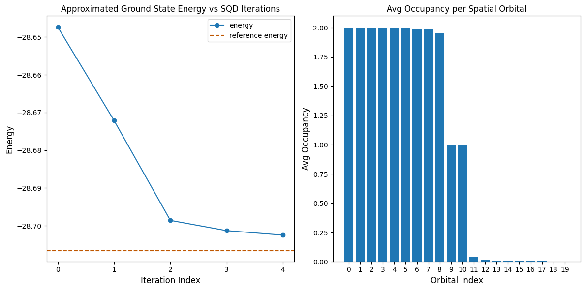
code cell ต่อไปนี้ plot ผลลัพธ์ plot แรกแสดง energy ที่คำนวณได้เป็นฟังก์ชันของจำนวน configuration recovery iteration และ plot ที่สองแสดง average occupancy ของแต่ละ spatial orbital หลังจาก iteration สุดท้าย สำหรับ reference energy เราใช้ผลลัพธ์จากการคำนวณ DMRG ที่ทำแยกต่างหาก

import matplotlib.pyplot as plt

dmrg_energy = -28.70659686

min_es = [
    min(result, key=lambda res: res.energy).energy
    for result in result_history
]
min_id, min_e = min(enumerate(min_es), key=lambda x: x[1])

# Data for energies plot
x1 = range(len(result_history))

# Data for avg spatial orbital occupancy
y2 = np.sum(result.orbital_occupancies, axis=0)
x2 = range(len(y2))

fig, axs = plt.subplots(1, 2, figsize=(12, 6))

# Plot energies
axs[0].plot(x1, min_es, label="energy", marker="o")
axs[0].set_xticks(x1)
axs[0].set_xticklabels(x1)
axs[0].axhline(
    y=dmrg_energy, color="#BF5700", linestyle="--", label="DMRG energy"
)
axs[0].set_title("Approximated Ground State Energy vs SQD Iterations")
axs[0].set_xlabel("Iteration Index", fontdict={"fontsize": 12})
axs[0].set_ylabel("Energy", fontdict={"fontsize": 12})
axs[0].legend()

# Plot orbital occupancy
axs[1].bar(x2, y2, width=0.8)
axs[1].set_xticks(x2)
axs[1].set_xticklabels(x2)
axs[1].set_title("Avg Occupancy per Spatial Orbital")
axs[1].set_xlabel("Orbital Index", fontdict={"fontsize": 12})
axs[1].set_ylabel("Avg Occupancy", fontdict={"fontsize": 12})

print(f"Reference (DMRG) energy: {dmrg_energy:.5f}")
print(f"SQD energy: {min_e:.5f}")
print(f"Absolute error: {abs(min_e - dmrg_energy):.5f}")
plt.tight_layout()
plt.show()

Reference (DMRG) energy: -28.70660
SQD energy: -28.69506
Absolute error: 0.01154

การตรวจสอบ energy

energy ที่ SQD คืนมารับประกันว่าเป็น upper bound ของ true ground state energy จริง ค่า energy สามารถตรวจสอบได้เพราะ SQD ยังคืน coefficient ของ state vector ที่ประมาณ ground state ด้วย เราสามารถคำนวณ energy จาก state vector โดยใช้ 1- และ 2-particle reduced density matrix ดังที่แสดงใน code cell ต่อไปนี้

rdm1 = result.sci_state.rdm(rank=1, spin_summed=True)
rdm2 = result.sci_state.rdm(rank=2, spin_summed=True)

energy = np.sum(h1e_momentum * rdm1) + 0.5 * np.sum(h2e_momentum * rdm2)

print(f"Recomputed energy: {energy:.5f}")

Recomputed energy: -28.69506

อ้างอิง

• Quantum-Centric Algorithm for Sample-Based Krylov Diagonalization (SKQD paper)
• Chemistry Beyond Exact Solutions on a Quantum-Centric Supercomputer (SQD paper)
• Diagonalization of large many-body Hamiltonians on a quantum processor (KQD paper)