อัลกอริทึมของ Shor

ประมาณการใช้งาน: สามวินาทีบนโปรเซสเซอร์ Eagle r3 (หมายเหตุ: นี่เป็นการประมาณเท่านั้น เวลาจริงอาจแตกต่างออกไป)

อัลกอริทึมของ Shor ที่พัฒนาโดย Peter Shor ในปี 1994 เป็นอัลกอริทึมควอนตัมที่ก้าวล้ำสำหรับการแยกตัวประกอบของจำนวนเต็มในเวลาแบบพหุนาม ความสำคัญของมันอยู่ที่ความสามารถในการแยกตัวประกอบของจำนวนเต็มขนาดใหญ่ได้เร็วกว่าอัลกอริทึมแบบคลาสสิกที่รู้จักใด ๆ แบบเอ็กซ์โพเนนเชียล ซึ่งคุกคามความปลอดภัยของระบบเข้ารหัสที่ใช้กันอย่างแพร่หลาย เช่น RSA ที่อาศัยความยากในการแยกตัวประกอบของจำนวนขนาดใหญ่ หากสามารถแก้ปัญหานี้ได้อย่างมีประสิทธิภาพบนคอมพิวเตอร์ควอนตัมที่มีประสิทธิภาพเพียงพอ อัลกอริทึมของ Shor อาจปฏิวัติสาขาต่าง ๆ เช่น การเข้ารหัส ความปลอดภัยทางไซเบอร์ และคณิตศาสตร์เชิงคำนวณ ซึ่งแสดงให้เห็นถึงพลังการเปลี่ยนแปลงของการคำนวณควอนตัม

บทช่วยสอนนี้มุ่งเน้นการสาธิตอัลกอริทึมของ Shor โดยการแยกตัวประกอบของ 15 บนคอมพิวเตอร์ควอนตัม

ขั้นแรก เรานิยามปัญหาการหาลำดับและสร้าง Circuit ที่สอดคล้องจากโปรโตคอลการประมาณเฟสควอนตัม ต่อมา เรารันวงจรการหาลำดับบนฮาร์ดแวร์จริงโดยใช้วงจรที่มีความลึกสั้นที่สุดที่เรา transpile ได้ ส่วนสุดท้ายจะทำให้อัลกอริทึมของ Shor สมบูรณ์โดยเชื่อมโยงปัญหาการหาลำดับกับการแยกตัวประกอบของจำนวนเต็ม

เราสิ้นสุดบทช่วยสอนด้วยการอภิปรายเกี่ยวกับการสาธิตอัลกอริทึมของ Shor บนฮาร์ดแวร์จริงอื่น ๆ โดยมุ่งเน้นทั้งการใช้งานทั่วไปและที่ปรับแต่งเพื่อแยกตัวประกอบของจำนวนเฉพาะ เช่น 15 และ 21 หมายเหตุ: บทช่วยสอนนี้เน้นการใช้งานและการสาธิต Circuit ที่เกี่ยวข้องกับอัลกอริทึมของ Shor มากกว่า สำหรับแหล่งเรียนรู้เชิงลึก โปรดดูที่คอร์ส Fundamentals of quantum algorithms โดย ดร. John Watrous และบทความในส่วน References

ความต้องการ

ก่อนเริ่มบทช่วยสอนนี้ ให้ตรวจสอบว่าคุณได้ติดตั้งสิ่งต่อไปนี้แล้ว:

• Qiskit SDK v2.0 หรือใหม่กว่า พร้อมรองรับ visualization
• Qiskit Runtime v0.40 หรือใหม่กว่า (pip install qiskit-ibm-runtime)

การตั้งค่า

# Added by doQumentation — required packages for this notebook
!pip install -q numpy pandas qiskit qiskit-ibm-runtime

import numpy as np
import pandas as pd
from fractions import Fraction
from math import floor, gcd, log

from qiskit import QuantumCircuit, QuantumRegister, ClassicalRegister
from qiskit.circuit.library import QFT, UnitaryGate
from qiskit.transpiler import CouplingMap, generate_preset_pass_manager
from qiskit.visualization import plot_histogram

from qiskit_ibm_runtime import QiskitRuntimeService
from qiskit_ibm_runtime import SamplerV2 as Sampler

ขั้นตอนที่ 1: แมปอินพุตแบบคลาสสิกไปยังปัญหาควอนตัม

พื้นฐาน

อัลกอริทึมของ Shor สำหรับการแยกตัวประกอบจำนวนเต็มใช้ปัญหาตัวกลางที่เรียกว่าปัญหา การหาลำดับ ในส่วนนี้ เราสาธิตวิธีแก้ปัญหาการหาลำดับโดยใช้ การประมาณเฟสควอนตัม

ปัญหาการประมาณเฟส

ในปัญหาการประมาณเฟส เราได้รับสถานะควอนตัม $\ket{\psi}$ ของ $n$ Qubit พร้อมกับ Circuit ควอนตัมยูนิทารีที่กระทำบน $n$ Qubit เราได้รับการรับรองว่า $\ket{\psi}$ เป็น eigenvector ของเมทริกซ์ยูนิทารี $U$ ที่อธิบายการกระทำของ Circuit และเป้าหมายของเราคือการคำนวณหรือประมาณ eigenvalue $\lambda = e^{2 \pi i \theta}$ ที่ $\ket{\psi}$ สอดคล้องกัน กล่าวอีกนัยหนึ่ง Circuit ควรให้ผลลัพธ์เป็นการประมาณค่าของตัวเลข $\theta \in [0, 1)$ ที่ตอบสนอง $U \ket{\psi}= e^{2 \pi i \theta} \ket{\psi}.$ เป้าหมายของ Circuit การประมาณเฟสคือการประมาณ $\theta$ ใน $m$ บิต ในแง่คณิตศาสตร์ เราต้องการหา $y$ ที่ $\theta \approx y / 2^m$ โดย $y \in {0, 1, 2, \dots, 2^{m-1}}$ ภาพต่อไปนี้แสดง Circuit ควอนตัมที่ประมาณ $y$ ใน $m$ บิต โดยทำการวัดบน $m$ Qubit

ใน Circuit ข้างต้น Qubit ด้านบน $m$ ตัวถูกเริ่มต้นในสถานะ $\ket{0^m}$ และ Qubit ด้านล่าง $n$ ตัวถูกเริ่มต้นใน $\ket{\psi}$ ซึ่งได้รับการรับรองว่าเป็น eigenvector ของ $U$ ส่วนประกอบแรกใน Circuit การประมาณเฟสคือการดำเนินการยูนิทารีแบบ controlled ที่รับผิดชอบในการทำ phase kickback ไปยัง control qubit ที่สอดคล้องกัน ยูนิทารีแบบ controlled เหล่านี้ถูกยกกำลังตามตำแหน่งของ control qubit ตั้งแต่บิตที่มีนัยสำคัญน้อยที่สุดไปจนถึงบิตที่มีนัยสำคัญมากที่สุด เนื่องจาก $\ket{\psi}$ เป็น eigenvector ของ $U$ สถานะของ Qubit ด้านล่าง $n$ ตัวจึงไม่ได้รับผลกระทบจากการดำเนินการนี้ แต่ข้อมูลเฟสของ eigenvalue จะแพร่กระจายไปยัง Qubit ด้านบน $m$ ตัว ปรากฏว่าหลังจากการดำเนินการ phase kickback ผ่านยูนิทารีแบบ controlled สถานะที่เป็นไปได้ทั้งหมดของ Qubit ด้านบน $m$ ตัวต่างเป็น orthonormal ซึ่งกันและกันสำหรับแต่ละ eigenvector $\ket{\psi}$ ของยูนิทารี $U$ ดังนั้น สถานะเหล่านี้จึงสามารถแยกแยะได้อย่างสมบูรณ์ และเราสามารถหมุนฐานที่สถานะเหล่านี้ก่อตัวกลับไปยังฐานการคำนวณเพื่อทำการวัด การวิเคราะห์ทางคณิตศาสตร์แสดงให้เห็นว่าเมทริกซ์การหมุนนี้สอดคล้องกับการแปลงฟูริเยร์ควอนตัมผกผัน (QFT) ในปริภูมิ Hilbert มิติ $2^m$ แนวคิดเบื้องหลังคือโครงสร้างเป็นคาบของตัวดำเนินการยกกำลังโมดูลาร์ถูกเข้ารหัสในสถานะควอนตัม และ QFT แปลงความเป็นคาบนี้ให้เป็นยอดที่วัดได้ในโดเมนความถี่

สำหรับความเข้าใจเชิงลึกยิ่งขึ้นว่าทำไม Circuit QFT จึงถูกนำมาใช้ในอัลกอริทึมของ Shor เราแนะนำให้ผู้อ่านดูที่คอร์ส Fundamentals of quantum algorithms ตอนนี้เราพร้อมที่จะใช้ Circuit การประมาณเฟสสำหรับการหาลำดับแล้ว

ปัญหาการหาลำดับ

เพื่อนิยามปัญหาการหาลำดับ เราเริ่มจากแนวคิดพื้นฐานของทฤษฎีจำนวน ก่อนอื่น สำหรับจำนวนเต็มบวก $N$ ใด ๆ ที่กำหนด ให้นิยามเซต $\mathbb{Z}_N$ เป็น $\mathbb{Z}_N = \{0, 1, 2, \dots, N-1\}.$ การดำเนินการทางคณิตศาสตร์ทั้งหมดใน $\mathbb{Z}_N$ ทำแบบโมดูโล $N$ โดยเฉพาะ สมาชิกทั้งหมด $a \in \mathbb{Z}_n$ ที่เป็นจำนวนเฉพาะสัมพัทธ์กับ $N$ เป็นพิเศษและประกอบขึ้นเป็น $\mathbb{Z}^*_N$ ดังนี้ $\mathbb{Z}^*_N = \{ a \in \mathbb{Z}_N : \mathrm{gcd}(a, N)=1 \}.$ สำหรับสมาชิก $a \in \mathbb{Z}^*_N$ จำนวนเต็มบวกที่เล็กที่สุด $r$ ที่ทำให้ $a^r \equiv 1 \; (\mathrm{mod} \; N)$ ถูกนิยามว่าเป็น ลำดับ ของ $a$ โมดูโล $N$ ดังที่เราจะเห็นในภายหลัง การหาลำดับของ $a \in \mathbb{Z}^*_N$ จะทำให้เราสามารถแยกตัวประกอบ $N$ ได้ เพื่อสร้าง Circuit การหาลำดับจาก Circuit การประมาณเฟส เราต้องพิจารณาสองอย่าง ประการแรก เราต้องนิยามยูนิทารี $U$ ที่จะช่วยให้เราหาลำดับ $r$ ได้ และประการที่สอง เราต้องนิยาม eigenvector $\ket{\psi}$ ของ $U$ เพื่อเตรียมสถานะเริ่มต้นของ Circuit การประมาณเฟส

เพื่อเชื่อมโยงปัญหาการหาลำดับกับการประมาณเฟส เราพิจารณาการดำเนินการที่นิยามบนระบบที่สถานะแบบคลาสสิกสอดคล้องกับ $\mathbb{Z}_N$ ซึ่งเราคูณด้วยสมาชิกคงที่ $a \in \mathbb{Z}^*_N$ โดยเฉพาะ เรานิยามตัวดำเนินการการคูณ $M_a$ ดังนี้ $M_a \ket{x} = \ket{ax \; (\mathrm{mod} \; N)}$ สำหรับแต่ละ $x \in \mathbb{Z}_N$ สังเกตว่าเป็นนัยว่าเราคำนวณผลคูณแบบโมดูโล $N$ ภายใน ket ด้านขวามือของสมการ การวิเคราะห์ทางคณิตศาสตร์แสดงให้เห็นว่า $M_a$ เป็นตัวดำเนินการยูนิทารี ยิ่งไปกว่านั้น ปรากฏว่า $M_a$ มีคู่ eigenvector และ eigenvalue ที่ทำให้เราเชื่อมโยงลำดับ $r$ ของ $a$ กับปัญหาการประมาณเฟสได้ โดยเฉพาะ สำหรับการเลือก $j \in \{0, \dots, r-1\}$ ใด ๆ เรามีว่า $\ket{\psi_j} = \frac{1}{\sqrt{r}} \sum^{r-1}_{k=0} \omega^{-jk}_{r} \ket{a^k}$ เป็น eigenvector ของ $M_a$ ที่มี eigenvalue ที่สอดคล้องกันเป็น $\omega^{j}_{r}$ โดยที่ $\omega^{j}_{r} = e^{2 \pi i \frac{j}{r}}.$ จากการสังเกต เราเห็นว่าคู่ eigenvector/eigenvalue ที่สะดวกคือสถานะ $\ket{\psi_1}$ ที่มี $\omega^{1}_{r} = e^{2 \pi i \frac{1}{r}}$ ดังนั้น ถ้าเราสามารถหา eigenvector $\ket{\psi_1}$ ได้ เราก็สามารถประมาณเฟส $\theta=1/r$ ด้วย Circuit ควอนตัมของเรา และจึงได้การประมาณลำดับ $r$ อย่างไรก็ตาม การทำเช่นนั้นไม่ใช่เรื่องง่าย และเราต้องพิจารณาทางเลือกอื่น

มาพิจารณาว่า Circuit จะให้ผลลัพธ์อะไรหากเราเตรียมสถานะการคำนวณ $\ket{1}$ เป็นสถานะเริ่มต้น นี่ไม่ใช่ eigenstate ของ $M_a$ แต่เป็นซูเปอร์โพสิชันสม่ำเสมอของ eigenstate ที่เราเพิ่งอธิบายไว้ กล่าวอีกนัยหนึ่ง ความสัมพันธ์ต่อไปนี้ถือเป็นจริง $\ket{1} = \frac{1}{\sqrt{r}} \sum^{r-1}_{k=0} \ket{\psi_k}$ ผลที่ตามมาของสมการข้างต้นคือ ถ้าเราตั้งสถานะเริ่มต้นเป็น $\ket{1}$ เราจะได้ผลการวัดที่เหมือนกันกับว่าเราเลือก $k \in \{ 0, \dots, r-1\}$ แบบสม่ำเสมอแบบสุ่มและใช้ $\ket{\psi_k}$ เป็น eigenvector ใน Circuit การประมาณเฟส กล่าวอีกนัยหนึ่ง การวัด Qubit ด้านบน $m$ ตัวให้การประมาณ $y / 2^m$ ของค่า $k / r$ โดย $k \in \{ 0, \dots, r-1\}$ ถูกเลือกแบบสม่ำเสมอแบบสุ่ม ซึ่งทำให้เราสามารถเรียนรู้ $r$ ด้วยความมั่นใจสูงหลังจากการรันอิสระหลายครั้ง ซึ่งเป็นเป้าหมายของเรา

ตัวดำเนินการยกกำลังโมดูลาร์

จนถึงตอนนี้ เราได้เชื่อมโยงปัญหาการประมาณเฟสกับปัญหาการหาลำดับโดยนิยาม $U = M_a$ และ $\ket{\psi} = \ket{1}$ ใน Circuit ควอนตัมของเรา ดังนั้น ส่วนประกอบสุดท้ายที่เหลืออยู่คือการหาวิธีที่มีประสิทธิภาพในการนิยามยกกำลังโมดูลาร์ของ $M_a$ เป็น $M_a^k$ สำหรับ $k = 1, 2, 4, \dots, 2^{m-1}$ เพื่อดำเนินการคำนวณนี้ เราพบว่าสำหรับกำลัง $k$ ใด ๆ ที่เราเลือก เราสามารถสร้าง Circuit สำหรับ $M_a^k$ ไม่ใช่โดยการวนซ้ำ Circuit สำหรับ $M_a$ จำนวน $k$ ครั้ง แต่แทนที่โดยการคำนวณ $b = a^k \; \mathrm{mod} \; N$ แล้วใช้ Circuit สำหรับ $M_b$ เนื่องจากเราต้องการเฉพาะกำลังที่เป็นกำลังของ 2 เราจึงสามารถทำสิ่งนี้ได้อย่างมีประสิทธิภาพแบบคลาสสิกโดยใช้การยกกำลังสองซ้ำ ๆ

ขั้นตอนที่ 2: ปรับปรุงปัญหาสำหรับการรันบนฮาร์ดแวร์ควอนตัม

ตัวอย่างเฉพาะกับ $N = 15$ และ $a=2$

เราสามารถหยุดพักที่นี่เพื่อพูดถึงตัวอย่างเฉพาะและสร้าง Circuit การหาลำดับสำหรับ $N=15$ สังเกตว่า $a \in \mathbb{Z}_N^*$ ที่ไม่ใช่ค่าพื้นฐานที่เป็นไปได้สำหรับ $N=15$ คือ $a \in \{2, 4, 7, 8, 11, 13, 14 \}$ สำหรับตัวอย่างนี้ เราเลือก $a=2$ เราจะสร้างตัวดำเนินการ $M_2$ และตัวดำเนินการยกกำลังโมดูลาร์ $M_2^k$ การกระทำของ $M_2$ บนสถานะฐานการคำนวณมีดังนี้ $M_2 \ket{0} = \ket{0} \quad M_2 \ket{5} = \ket{10} \quad M_2 \ket{10} = \ket{5}$ $M_2 \ket{1} = \ket{2} \quad M_2 \ket{6} = \ket{12} \quad M_2 \ket{11} = \ket{7}$ $M_2 \ket{2} = \ket{4} \quad M_2 \ket{7} = \ket{14} \quad M_2 \ket{12} = \ket{9}$ $M_2 \ket{3} = \ket{6} \quad M_2 \ket{8} = \ket{1} \quad M_2 \ket{13} = \ket{11}$ $M_2 \ket{4} = \ket{8} \quad M_2 \ket{9} = \ket{3} \quad M_2 \ket{14} = \ket{13}$ จากการสังเกต เราเห็นว่าสถานะฐานถูกสลับ ดังนั้นเราจึงมีเมทริกซ์การเรียงสับเปลี่ยน เราสามารถสร้างการดำเนินการนี้บนสี่ Qubit ด้วย swap gate ด้านล่าง เราสร้างการดำเนินการ $M_2$ และ controlled-$M_2$

def M2mod15():
    """
    M2 (mod 15)
    """
    b = 2
    U = QuantumCircuit(4)

    U.swap(2, 3)
    U.swap(1, 2)
    U.swap(0, 1)

    U = U.to_gate()
    U.name = f"M_{b}"

    return U

# Get the M2 operator
M2 = M2mod15()

# Add it to a circuit and plot
circ = QuantumCircuit(4)
circ.compose(M2, inplace=True)
circ.decompose(reps=2).draw(output="mpl", fold=-1)

def controlled_M2mod15():
    """
    Controlled M2 (mod 15)
    """
    b = 2
    U = QuantumCircuit(4)

    U.swap(2, 3)
    U.swap(1, 2)
    U.swap(0, 1)

    U = U.to_gate()
    U.name = f"M_{b}"
    c_U = U.control()

    return c_U

# Get the controlled-M2 operator
controlled_M2 = controlled_M2mod15()

# Add it to a circuit and plot
circ = QuantumCircuit(5)
circ.compose(controlled_M2, inplace=True)
circ.decompose(reps=1).draw(output="mpl", fold=-1)

Gate ที่กระทำบน Qubit มากกว่าสองตัวจะถูก decompose เพิ่มเติมเป็น two-qubit gate

circ.decompose(reps=2).draw(output="mpl", fold=-1)

ตอนนี้เราต้องสร้างตัวดำเนินการยกกำลังโมดูลาร์ เพื่อให้ได้ความแม่นยำเพียงพอในการประมาณเฟส เราจะใช้ Qubit แปดตัวสำหรับการวัดประมาณ ดังนั้น เราต้องสร้าง $M_b$ ที่มี $b = a^{2^k} \; (\mathrm{mod} \; N)$ สำหรับแต่ละ $k = 0, 1, \dots, 7$

def a2kmodN(a, k, N):
    """Compute a^{2^k} (mod N) by repeated squaring"""
    for _ in range(k):
        a = int(np.mod(a**2, N))
    return a

k_list = range(8)
b_list = [a2kmodN(2, k, 15) for k in k_list]

print(b_list)

[2, 4, 1, 1, 1, 1, 1, 1]

จากรายการค่า $b$ ที่เห็น นอกจาก $M_2$ ที่เราสร้างไว้ก่อนหน้านี้ เรายังต้องสร้าง $M_4$ และ $M_1$ ด้วย สังเกตว่า $M_1$ กระทำอย่างไม่มีนัยสำคัญบนสถานะฐานการคำนวณ ดังนั้นมันเป็นเพียงตัวดำเนินการเอกลักษณ์

$M_4$ กระทำบนสถานะฐานการคำนวณดังนี้ $M_4 \ket{0} = \ket{0} \quad M_4 \ket{5} = \ket{5} \quad M_4 \ket{10} = \ket{10}$ $M_4 \ket{1} = \ket{4} \quad M_4 \ket{6} = \ket{9} \quad M_4 \ket{11} = \ket{14}$ $M_4 \ket{2} = \ket{8} \quad M_4 \ket{7} = \ket{13} \quad M_4 \ket{12} = \ket{3}$ $M_4 \ket{3} = \ket{12} \quad M_4 \ket{8} = \ket{2} \quad M_4 \ket{13} = \ket{7}$ $M_4 \ket{4} = \ket{1} \quad M_4 \ket{9} = \ket{6} \quad M_4 \ket{14} = \ket{11}$

ดังนั้น การเรียงสับเปลี่ยนนี้สามารถสร้างได้ด้วยการดำเนินการ swap ต่อไปนี้

def M4mod15():
    """
    M4 (mod 15)
    """
    b = 4
    U = QuantumCircuit(4)

    U.swap(1, 3)
    U.swap(0, 2)

    U = U.to_gate()
    U.name = f"M_{b}"

    return U

# Get the M4 operator
M4 = M4mod15()

# Add it to a circuit and plot
circ = QuantumCircuit(4)
circ.compose(M4, inplace=True)
circ.decompose(reps=2).draw(output="mpl", fold=-1)

def controlled_M4mod15():
    """
    Controlled M4 (mod 15)
    """
    b = 4
    U = QuantumCircuit(4)

    U.swap(1, 3)
    U.swap(0, 2)

    U = U.to_gate()
    U.name = f"M_{b}"
    c_U = U.control()

    return c_U

# Get the controlled-M4 operator
controlled_M4 = controlled_M4mod15()

# Add it to a circuit and plot
circ = QuantumCircuit(5)
circ.compose(controlled_M4, inplace=True)
circ.decompose(reps=1).draw(output="mpl", fold=-1)

Gate ที่กระทำบน Qubit มากกว่าสองตัวจะถูก decompose เพิ่มเติมเป็น two-qubit gate

circ.decompose(reps=2).draw(output="mpl", fold=-1)

เราเห็นว่าตัวดำเนินการ $M_b$ สำหรับ $b \in \mathbb{Z}^*_N$ ที่กำหนดเป็นการดำเนินการเรียงสับเปลี่ยน เนื่องจากขนาดค่อนข้างเล็กของปัญหาการเรียงสับเปลี่ยนที่เรามีที่นี่ เนื่องจาก $N=15$ ต้องการเพียงสี่ Qubit เราจึงสามารถสังเคราะห์การดำเนินการเหล่านี้ได้โดยตรงด้วย SWAP gate โดยการสังเกต โดยทั่วไปแล้ว แนวทางนี้อาจไม่สามารถขยายขนาดได้ แต่เราอาจต้องสร้างเมทริกซ์การเรียงสับเปลี่ยนอย่างชัดเจน และใช้คลาส UnitaryGate ของ Qiskit และวิธีการ transpile เพื่อสังเคราะห์เมทริกซ์การเรียงสับเปลี่ยนนี้ อย่างไรก็ตาม สิ่งนี้อาจส่งผลให้ Circuit มีความลึกมากขึ้นอย่างมีนัยสำคัญ ต่อไปนี้คือตัวอย่าง

def mod_mult_gate(b, N):
    """
    Modular multiplication gate from permutation matrix.
    """
    if gcd(b, N) > 1:
        print(f"Error: gcd({b},{N}) > 1")
    else:
        n = floor(log(N - 1, 2)) + 1
        U = np.full((2**n, 2**n), 0)
        for x in range(N):
            U[b * x % N][x] = 1
        for x in range(N, 2**n):
            U[x][x] = 1
        G = UnitaryGate(U)
        G.name = f"M_{b}"
        return G

# Let's build M2 using the permutation matrix definition
M2_other = mod_mult_gate(2, 15)

# Add it to a circuit
circ = QuantumCircuit(4)
circ.compose(M2_other, inplace=True)
circ = circ.decompose()

# Transpile the circuit and get the depth
coupling_map = CouplingMap.from_line(4)
pm = generate_preset_pass_manager(coupling_map=coupling_map)
transpiled_circ = pm.run(circ)

print(f"qubits: {circ.num_qubits}")
print(
    f"2q-depth: {transpiled_circ.depth(lambda x: x.operation.num_qubits==2)}"
)
print(f"2q-size: {transpiled_circ.size(lambda x: x.operation.num_qubits==2)}")
print(f"Operator counts: {transpiled_circ.count_ops()}")
transpiled_circ.decompose().draw(
    output="mpl", fold=-1, style="clifford", idle_wires=False
)

qubits: 4
2q-depth: 94
2q-size: 96
Operator counts: OrderedDict({'cx': 45, 'swap': 32, 'u': 24, 'u1': 7, 'u3': 4, 'unitary': 3, 'circuit-335': 1, 'circuit-338': 1, 'circuit-341': 1, 'circuit-344': 1, 'circuit-347': 1, 'circuit-350': 1, 'circuit-353': 1, 'circuit-356': 1, 'circuit-359': 1, 'circuit-362': 1, 'circuit-365': 1, 'circuit-368': 1, 'circuit-371': 1, 'circuit-374': 1, 'circuit-377': 1, 'circuit-380': 1})

มาเปรียบเทียบจำนวนเหล่านี้กับความลึกของ Circuit ที่คอมไพล์แล้วของการใช้งาน $M_2$ gate แบบแมนนวลของเรา

# Get the M2 operator from our manual construction
M2 = M2mod15()

# Add it to a circuit
circ = QuantumCircuit(4)
circ.compose(M2, inplace=True)
circ = circ.decompose(reps=3)

# Transpile the circuit and get the depth
coupling_map = CouplingMap.from_line(4)
pm = generate_preset_pass_manager(coupling_map=coupling_map)
transpiled_circ = pm.run(circ)

print(f"qubits: {circ.num_qubits}")
print(
    f"2q-depth: {transpiled_circ.depth(lambda x: x.operation.num_qubits==2)}"
)
print(f"2q-size: {transpiled_circ.size(lambda x: x.operation.num_qubits==2)}")
print(f"Operator counts: {transpiled_circ.count_ops()}")
transpiled_circ.draw(
    output="mpl", fold=-1, style="clifford", idle_wires=False
)

qubits: 4
2q-depth: 9
2q-size: 9
Operator counts: OrderedDict({'cx': 9})

จากที่เห็น แนวทางเมทริกซ์การเรียงสับเปลี่ยนส่งผลให้ Circuit มีความลึกมากอย่างมีนัยสำคัญแม้แต่สำหรับ $M_2$ gate เดียว เมื่อเปรียบเทียบกับการใช้งานแบบแมนนวลของเรา ดังนั้น เราจะดำเนินการต่อด้วยการใช้งานก่อนหน้าของเราสำหรับการดำเนินการ $M_b$ ตอนนี้ เราพร้อมที่จะสร้าง Circuit การหาลำดับเต็มรูปแบบโดยใช้ตัวดำเนินการยกกำลังโมดูลาร์แบบ controlled ที่นิยามไว้ก่อนหน้า ในโค้ดต่อไปนี้ เรายังนำเข้า QFT circuit จาก Qiskit Circuit library ซึ่งใช้ Hadamard gate บนแต่ละ Qubit, ชุดของ controlled-U1 (หรือ Z ขึ้นอยู่กับเฟส) gate และชั้นของ swap gate

# Order finding problem for N = 15 with a = 2
N = 15
a = 2

# Number of qubits
num_target = floor(log(N - 1, 2)) + 1  # for modular exponentiation operators
num_control = 2 * num_target  # for enough precision of estimation

# List of M_b operators in order
k_list = range(num_control)
b_list = [a2kmodN(2, k, 15) for k in k_list]

# Initialize the circuit
control = QuantumRegister(num_control, name="C")
target = QuantumRegister(num_target, name="T")
output = ClassicalRegister(num_control, name="out")
circuit = QuantumCircuit(control, target, output)

# Initialize the target register to the state |1>
circuit.x(num_control)

# Add the Hadamard gates and controlled versions of the
# multiplication gates
for k, qubit in enumerate(control):
    circuit.h(k)
    b = b_list[k]
    if b == 2:
        circuit.compose(
            M2mod15().control(), qubits=[qubit] + list(target), inplace=True
        )
    elif b == 4:
        circuit.compose(
            M4mod15().control(), qubits=[qubit] + list(target), inplace=True
        )
    else:
        continue  # M1 is the identity operator

# Apply the inverse QFT to the control register
circuit.compose(QFT(num_control, inverse=True), qubits=control, inplace=True)

# Measure the control register
circuit.measure(control, output)

circuit.draw("mpl", fold=-1)

สังเกตว่าเราละเว้นการดำเนินการยกกำลังโมดูลาร์แบบ controlled จาก control qubit ที่เหลือ เนื่องจาก $M_1$ เป็นตัวดำเนินการเอกลักษณ์ สังเกตว่าในภายหลังในบทช่วยสอนนี้ เราจะรัน Circuit นี้บน Backend ibm_marrakesh เพื่อทำสิ่งนี้ เรา transpile Circuit ตาม Backend เฉพาะนี้และรายงานความลึกของ Circuit และจำนวน gate

service = QiskitRuntimeService()
backend = service.backend("ibm_marrakesh")
pm = generate_preset_pass_manager(optimization_level=2, backend=backend)

transpiled_circuit = pm.run(circuit)

print(
    f"2q-depth: {transpiled_circuit.depth(lambda x: x.operation.num_qubits==2)}"
)
print(
    f"2q-size: {transpiled_circuit.size(lambda x: x.operation.num_qubits==2)}"
)
print(f"Operator counts: {transpiled_circuit.count_ops()}")
transpiled_circuit.draw(
    output="mpl", fold=-1, style="clifford", idle_wires=False
)

2q-depth: 187
2q-size: 260
Operator counts: OrderedDict({'sx': 521, 'rz': 354, 'cz': 260, 'measure': 8, 'x': 4})

ขั้นตอนที่ 3: รันด้วย Qiskit primitives

ก่อนอื่น มาดูกันว่าถ้าเราเอา Circuit นี้ไปรันบน simulator อุดมคติจะได้ผลอะไรในทางทฤษฎี ด้านล่างคือผลการ simulate Circuit ข้างต้นด้วย 1024 shots จะเห็นว่าได้การแจกแจงที่เกือบสม่ำเสมอกระจายอยู่บน bitstring สี่แบบในส่วน control qubits

# Obtained from the simulator
counts = {"00000000": 264, "01000000": 268, "10000000": 249, "11000000": 243}

plot_histogram(counts)

การวัด control qubits ทำให้เราได้ค่า phase estimation แบบแปดบิตของ operator $M_a$ เราสามารถแปลงจาก binary เป็น decimal เพื่อหาค่า phase ที่วัดได้ ดังที่เห็นในฮิสโตแกรมข้างต้น มี bitstring สี่แบบที่ถูกวัดได้ แต่ละแบบสอดคล้องกับค่า phase ดังนี้

# Rows to be displayed in table
rows = []
# Corresponding phase of each bitstring
measured_phases = []

for output in counts:
    decimal = int(output, 2)  # Convert bitstring to decimal
    phase = decimal / (2**num_control)  # Find corresponding eigenvalue
    measured_phases.append(phase)
    # Add these values to the rows in our table:
    rows.append(
        [
            f"{output}(bin) = {decimal:>3}(dec)",
            f"{decimal}/{2 ** num_control} = {phase:.2f}",
        ]
    )

# Print the rows in a table
headers = ["Register Output", "Phase"]
df = pd.DataFrame(rows, columns=headers)
print(df)

Register Output           Phase
0  00000000(bin) =   0(dec)    0/256 = 0.00
1  01000000(bin) =  64(dec)   64/256 = 0.25
2  10000000(bin) = 128(dec)  128/256 = 0.50
3  11000000(bin) = 192(dec)  192/256 = 0.75

ขอให้นึกถึงว่า ค่า phase ที่วัดได้ใดๆ จะสอดคล้องกับ $\theta = k / r$ โดยที่ $k$ ถูกสุ่มเลือกอย่างสม่ำเสมอจาก $\{0, 1, \dots, r-1 \}$ ดังนั้นเราสามารถใช้ algorithmen continued fractions เพื่อพยายามหา $k$ และ order $r$ Python มีฟังก์ชันนี้อยู่ในตัว เราสามารถใช้ module fractions เพื่อแปลง float เป็น object Fraction เช่น:

Fraction(0.666)

Fraction(5998794703657501, 9007199254740992)

เนื่องจากวิธีนี้จะให้ fraction ที่ตรงกับผลลัพธ์พอดี (ในกรณีนี้คือ 0.6660000...) ซึ่งอาจให้ผลลัพธ์ที่ยุ่งเหยิงอย่างตัวอย่างข้างต้น เราสามารถใช้ method .limit_denominator() เพื่อหา fraction ที่ใกล้เคียงกับ float ที่สุด โดยมีตัวส่วนต่ำกว่าค่าที่กำหนด:

# Get fraction that most closely resembles 0.666
# with denominator < 15
Fraction(0.666).limit_denominator(15)

Fraction(2, 3)

แบบนี้ดูดีกว่ามาก order (r) ต้องมีค่าน้อยกว่า N ดังนั้นเราจะกำหนดตัวส่วนสูงสุดไว้ที่ 15:

# Rows to be displayed in a table
rows = []

for phase in measured_phases:
    frac = Fraction(phase).limit_denominator(15)
    rows.append(
        [phase, f"{frac.numerator}/{frac.denominator}", frac.denominator]
    )

# Print the rows in a table
headers = ["Phase", "Fraction", "Guess for r"]
df = pd.DataFrame(rows, columns=headers)
print(df)

Phase Fraction  Guess for r
0   0.00      0/1            1
1   0.25      1/4            4
2   0.50      1/2            2
3   0.75      3/4            4

จะเห็นว่าค่า eigenvalue สองค่าที่วัดได้ให้ผลลัพธ์ที่ถูกต้อง: $r=4$ และสังเกตได้ว่า Shor's algorithm สำหรับการหา order มีโอกาสที่จะล้มเหลว ผลลัพธ์ที่ไม่ดีเหล่านี้เกิดจาก $k = 0$ หรือ $k$ กับ $r$ ไม่ coprime กัน ทำให้แทนที่จะได้ $r$ กลับได้ตัวประกอบของ $r$ แทน วิธีแก้ง่ายๆ คือรันการทดลองซ้ำจนกว่าจะได้ผลลัพธ์ $r$ ที่น่าพอใจ

จนถึงตอนนี้ เราได้ implement ปัญหาการหา order สำหรับ $N=15$ และ $a=2$ โดยใช้ phase estimation Circuit บน simulator แล้ว ขั้นตอนสุดท้ายของ Shor's algorithm คือการเชื่อมโยงปัญหาการหา order กับปัญหาการแยกตัวประกอบจำนวนเต็ม ส่วนสุดท้ายของ algorithm นี้เป็นแบบ classical ล้วนๆ และสามารถแก้บนคอมพิวเตอร์ classical ได้หลังจากได้ค่าการวัด phase มาจากคอมพิวเตอร์ quantum แล้ว ดังนั้นเราจะเลื่อนส่วนสุดท้ายของ algorithm ออกไปก่อน แล้วค่อยมาทำหลังจากที่เราแสดงวิธีรัน Circuit การหา order บน hardware จริง

การรันบน Hardware

ตอนนี้เราสามารถรัน Circuit การหา order ที่ transpile สำหรับ ibm_marrakesh ไว้แล้วได้เลย เราจะใช้ dynamical decoupling (DD) สำหรับการระงับ error และ gate twirling สำหรับการลด error DD คือการใช้ลำดับ control pulse ที่จับเวลาอย่างแม่นยำกับอุปกรณ์ quantum เพื่อหักล้างการรบกวนจากสภาพแวดล้อมและ decoherence ที่ไม่ต้องการออกอย่างมีประสิทธิภาพ ส่วน gate twirling จะสุ่ม gate quantum เฉพาะเพื่อแปลง coherent errors ให้เป็น Pauli errors ซึ่งสะสมแบบ linear แทนที่จะเป็น quadratic การใช้ทั้งสองเทคนิคพร้อมกันมักช่วยเพิ่ม coherence และ fidelity ของการคำนวณ quantum

# Sampler primitive to obtain the probability distribution
sampler = Sampler(backend)

# Turn on dynamical decoupling with sequence XpXm
sampler.options.dynamical_decoupling.enable = True
sampler.options.dynamical_decoupling.sequence_type = "XpXm"
# Enable gate twirling
sampler.options.twirling.enable_gates = True

pub = transpiled_circuit
job = sampler.run([pub], shots=1024)

result = job.result()[0]
counts = result.data["out"].get_counts()

plot_histogram(counts, figsize=(35, 5))

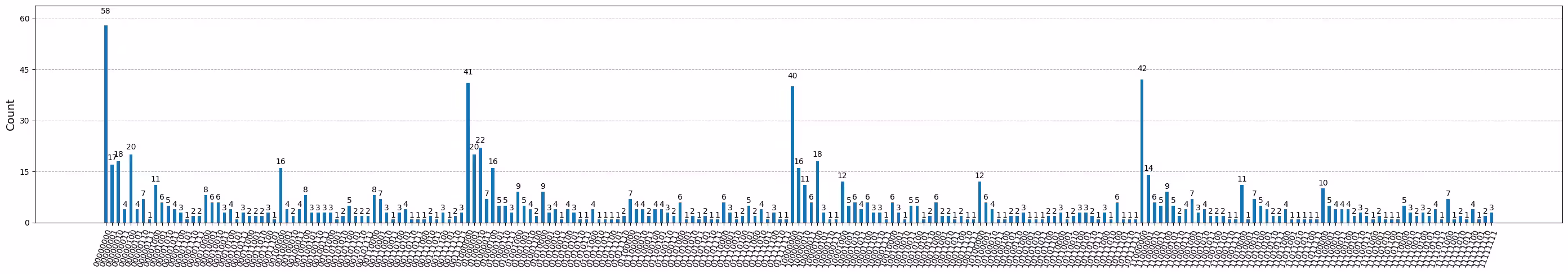
จะเห็นว่าเราได้ bitstring เดิมที่มีจำนวน count สูงสุด เนื่องจาก hardware quantum มี noise จึงมีการรั่วไหลไปยัง bitstring อื่น ซึ่งเราสามารถกรองออกได้ด้วยสถิติ

# Dictionary of bitstrings and their counts to keep
counts_keep = {}
# Threshold to filter
threshold = np.max(list(counts.values())) / 2

for key, value in counts.items():
    if value > threshold:
        counts_keep[key] = value

print(counts_keep)

{'00000000': 58, '01000000': 41, '11000000': 42, '10000000': 40}

ขั้นตอนที่ 4: Post-process และแสดงผลลัพธ์ในรูปแบบ classical ที่ต้องการ

การแยกตัวประกอบจำนวนเต็ม

จนถึงตอนนี้ เราได้พูดถึงวิธี implement ปัญหาการหา order โดยใช้ phase estimation Circuit แล้ว ตอนนี้เราจะเชื่อมโยงปัญหาการหา order กับการแยกตัวประกอบจำนวนเต็ม ซึ่งเป็นการทำให้ Shor's algorithm สมบูรณ์ ขอให้สังเกตว่าส่วนนี้ของ algorithm เป็น classical ล้วนๆ

ตอนนี้เราจะสาธิตโดยใช้ตัวอย่าง $N = 15$ และ $a = 2$ ขอให้นึกถึงว่า phase ที่วัดได้คือ $k / r$ โดยที่ $a^r \; (\textrm{mod} \; N) = 1$ และ $k$ คือจำนวนเต็มสุ่มระหว่าง $0$ ถึง $r - 1$ จากสมการนี้ เราได้ว่า $(a^r - 1) \; (\textrm{mod} \; N) = 0,$ ซึ่งหมายความว่า $N$ ต้องหาร $a^r-1$ ลงตัว ถ้า $r$ เป็นเลขคู่ด้วย เราสามารถเขียนได้ว่า $a^r -1 = (a^{r/2}-1)(a^{r/2}+1).$ ถ้า $r$ ไม่เป็นเลขคู่ เราไม่สามารถดำเนินการต่อได้และต้องลองใหม่ด้วยค่า $a$ ที่ต่างกัน มิฉะนั้น จะมีความน่าจะเป็นสูงที่ greatest common divisor ของ $N$ กับ $a^{r/2}-1$ หรือ $a^{r/2}+1$ จะเป็นตัวประกอบที่แท้จริงของ $N$

เนื่องจากการรัน algorithm บางครั้งจะล้มเหลวในทางสถิติ เราจะทำซ้ำ algorithm นี้จนกว่าจะพบตัวประกอบหนึ่งตัวของ $N$ อย่างน้อย

Cell ด้านล่างจะทำซ้ำ algorithm จนกว่าจะพบตัวประกอบหนึ่งตัวของ $N=15$ อย่างน้อย เราจะใช้ผลลัพธ์จากการรันบน hardware ข้างต้นเพื่อเดา phase และตัวประกอบที่สอดคล้องในแต่ละ iteration

a = 2
N = 15

FACTOR_FOUND = False
num_attempt = 0

while not FACTOR_FOUND:
    print(f"\nATTEMPT {num_attempt}:")
    # Here, we get the bitstring by iterating over outcomes
    # of a previous hardware run with multiple shots.
    # Instead, we can also perform a single-shot measurement
    # here in the loop.
    bitstring = list(counts_keep.keys())[num_attempt]
    num_attempt += 1
    # Find the phase from measurement
    decimal = int(bitstring, 2)
    phase = decimal / (2**num_control)  # phase = k / r
    print(f"Phase: theta = {phase}")

    # Guess the order from phase
    frac = Fraction(phase).limit_denominator(N)
    r = frac.denominator  # order = r
    print(f"Order of {a} modulo {N} estimated as: r = {r}")

    if phase != 0:
        # Guesses for factors are gcd(a^{r / 2} ± 1, 15)
        if r % 2 == 0:
            x = pow(a, r // 2, N) - 1
            d = gcd(x, N)
            if d > 1:
                FACTOR_FOUND = True
                print(f"*** Non-trivial factor found: {x} ***")

ATTEMPT 0:
Phase: theta = 0.0
Order of 2 modulo 15 estimated as: r = 1

ATTEMPT 1:
Phase: theta = 0.25
Order of 2 modulo 15 estimated as: r = 4
*** Non-trivial factor found: 3 ***

การอภิปราย

งานวิจัยที่เกี่ยวข้อง

ในส่วนนี้ เราจะพูดถึงงานวิจัยสำคัญอื่นๆ ที่ได้แสดงการใช้งาน Shor's algorithm บน hardware จริง

งานสำคัญ [3] จาก IBM® ได้สาธิต Shor's algorithm เป็นครั้งแรก โดยแยกตัวประกอบจำนวน 15 ออกเป็น 3 และ 5 ซึ่งเป็นตัวประกอบเฉพาะ โดยใช้คอมพิวเตอร์ quantum แบบ nuclear magnetic resonance (NMR) ขนาดเจ็ด Qubit การทดลองอีกชิ้น [4] แยกตัวประกอบ 15 โดยใช้ photonic qubits ด้วยการใช้ Qubit เดียวซ้ำหลายครั้งและเข้ารหัส work register ในสถานะมิติสูง นักวิจัยลดจำนวน Qubit ที่ต้องการเหลือหนึ่งในสามของ protocol มาตรฐาน โดยใช้ two-photon compiled algorithm งานสำคัญอีกชิ้นในการสาธิต Shor's algorithm คือ [5] ซึ่งใช้เทคนิค iterative phase estimation ของ Kitaev [8] เพื่อลดความต้องการ Qubit ของ algorithm ผู้เขียนใช้ control qubits เจ็ดตัวและ cache qubits สี่ตัว พร้อมกับการ implement modular multipliers อย่างไรก็ตาม การ implement นี้ต้องการการวัด mid-circuit พร้อม feed-forward operations และการนำ Qubit กลับมาใช้ใหม่พร้อม reset operations การสาธิตนี้ทำบนคอมพิวเตอร์ quantum แบบ ion-trap

งานวิจัยล่าสุดกว่า [6] มุ่งเน้นการแยกตัวประกอบ 15, 21, และ 35 บน hardware ของ IBM Quantum® คล้ายกับงานก่อนหน้า นักวิจัยใช้ version ที่ compile แล้วของ algorithm ซึ่งใช้ semi-classical quantum Fourier transform ตามที่ Kitaev เสนอเพื่อลดจำนวน physical qubits และ gate งานล่าสุดอีกชิ้น [7] ยังได้สาธิต proof-of-concept สำหรับการแยกตัวประกอบจำนวนเต็ม 21 ด้วย การสาธิตนี้ยังเกี่ยวข้องกับการใช้ version ที่ compile แล้วของ quantum phase estimation routine และต่อยอดจากการสาธิตก่อนหน้าโดย [4] ผู้เขียนก้าวไปไกลกว่างานนั้นด้วยการใช้ configuration ของ approximate Toffoli gates พร้อม residual phase shifts Algorithm นี้ถูก implement บน IBM quantum processors โดยใช้เพียงห้า Qubit และยืนยันการมีอยู่ของ entanglement ระหว่าง control และ register qubits ได้สำเร็จ

การ scale ของ algorithm

ขอให้สังเกตว่า RSA encryption มักใช้ขนาด key ในระดับ 2048 ถึง 4096 บิต การพยายามแยกตัวประกอบจำนวน 2048 บิตด้วย Shor's algorithm จะส่งผลให้ได้ quantum Circuit ที่มี Qubit หลายล้านตัว รวมถึง overhead ของ error correction และ circuit depth ในระดับพันล้าน ซึ่งเกินขีดความสามารถของ hardware quantum ปัจจุบัน ดังนั้น Shor's algorithm จะต้องอาศัยวิธีการสร้าง Circuit ที่ปรับปรุงให้เหมาะสมหรือ quantum error correction ที่แข็งแกร่งเพื่อให้ใช้งานได้จริงในการทำลายระบบ cryptographic สมัยใหม่ เราขอแนะนำ [9] สำหรับการอภิปรายที่ละเอียดกว่าเกี่ยวกับการประมาณทรัพยากรสำหรับ Shor's algorithm

ความท้าทาย

ขอแสดงความยินดีที่เรียนจบ tutorial นี้แล้ว! นี่เป็นเวลาที่ดีในการทดสอบความเข้าใจ ลองสร้าง Circuit สำหรับการแยกตัวประกอบ 21 ดูได้ไหม? เลือกค่า $a$ ที่ต้องการได้เลย จะต้องตัดสินใจเรื่องความแม่นยำของ bit ของ algorithm เพื่อเลือกจำนวน Qubit และจะต้องออกแบบ operator modular exponentiation $M_a$ เราสนับสนุนให้ลองทำด้วยตัวเอง แล้วค่อยอ่านเกี่ยวกับวิธีการที่แสดงในรูปที่ 9 ของ [6] และรูปที่ 2 ของ [7]

def M_a_mod21():
    """
    M_a (mod 21)
    """

    # Your code here
    pass

อ้างอิง

1. Shor, Peter W. "Polynomial-time algorithms for prime factorization and discrete logarithms on a quantum computer." SIAM review 41.2 (1999): 303-332.
2. IBM Quantum Fundamentals of Quantum Algorithms course by Dr. John Watrous.
3. Vandersypen, Lieven MK, et al. "Experimental realization of Shor's quantum factoring algorithm using nuclear magnetic resonance." Nature 414.6866 (2001): 883-887.
4. Martin-Lopez, Enrique, et al. "Experimental realization of Shor's quantum factoring algorithm using qubit recycling." Nature photonics 6.11 (2012): 773-776.
5. Monz, Thomas, et al. "Realization of a scalable Shor algorithm." Science 351.6277 (2016): 1068-1070.
6. Amico, Mirko, Zain H. Saleem, and Muir Kumph. "Experimental study of Shor's factoring algorithm using the IBM Q Experience." Physical Review A 100.1 (2019): 012305.
7. Skosana, Unathi, and Mark Tame. "Demonstration of Shor's factoring algorithm for N=21 on IBM quantum processors." Scientific reports 11.1 (2021): 16599.
8. Kitaev, A. Yu. "Quantum measurements and the Abelian stabilizer problem." arXiv preprint quant-ph/9511026 (1995).
9. Gidney, Craig, and Martin Ekerå. "How to factor 2048 bit RSA integers in 8 hours using 20 million noisy qubits." Quantum 5 (2021): 433.