การเข้ารหัสความสัมพันธ์ Pauli เพื่อลดความต้องการ max-cut

ประมาณการใช้งาน: 35 นาทีบนโปรเซสเซอร์ Eagle r3 (หมายเหตุ: นี่เป็นเพียงการประมาณเท่านั้น ระยะเวลาจริงอาจแตกต่างกันไป)

ผลลัพธ์การเรียนรู้

เข้าใจหลักการทางทฤษฎีเบื้องหลัง Pauli Correlation Encoding (PCE) รวมถึงวิธีที่ Pauli string แบบหลายวัตถุช่วยให้เกิดการบีบอัดเชิงพหุนามของปัญหาการปรับแต่งแบบคลาสสิก
นำ PCE ไปใช้จริงเพื่อเข้ารหัสและแก้ปัญหาการปรับแต่งขนาดใหญ่บนฮาร์ดแวร์ควอนตัมระยะใกล้

ข้อกำหนดเบื้องต้น

พื้นหลัง

บทแนะนำนี้นำเสนอ Pauli Correlation Encoding (PCE) [1] ซึ่งเป็นแนวทางที่ออกแบบมาเพื่อเข้ารหัสปัญหาการปรับแต่งให้เหมาะสมลงใน Qubit ได้อย่างมีประสิทธิภาพมากขึ้นสำหรับการคำนวณเชิงควอนตัม PCE แมปตัวแปรคลาสสิกในปัญหาการปรับแต่งไปยังความสัมพันธ์ของ Pauli-matrix แบบหลายวัตถุ ส่งผลให้เกิดการบีบอัดเชิงพหุนามของข้อกำหนดพื้นที่ของปัญหา การใช้ PCE ช่วยลดจำนวน Qubit ที่จำเป็นสำหรับการเข้ารหัส ทำให้มีประโยชน์อย่างยิ่งสำหรับอุปกรณ์ควอนตัมระยะใกล้ที่มีทรัพยากร Qubit จำกัด นอกจากนี้ยังมีการพิสูจน์เชิงวิเคราะห์ว่า PCE มีคุณสมบัติในการบรรเทา barren plateaus ในตัวเอง โดยมีความยืดหยุ่นแบบ super-polynomial ต่อปรากฏการณ์นี้ คุณสมบัติที่มีอยู่แล้วนี้ช่วยให้ตัวแก้ปัญหาการปรับแต่งเชิงควอนตัมมีประสิทธิภาพที่ไม่เคยมีมาก่อน

ภาพรวม

แนวทาง PCE ประกอบด้วยสามขั้นตอนหลัก ดังที่แสดงในรูปที่ 1 จาก [1] ด้านล่างนี้:

เข้ารหัสปัญหาการปรับแต่งลงใน Pauli correlation space
แก้ปัญหาโดยใช้ตัวแก้ปัญหาการปรับแต่งแบบควอนตัม-คลาสสิก
ถอดรหัสคำตอบกลับสู่พื้นที่การปรับแต่งเดิม แนวทาง PCE นี้สามารถปรับใช้ได้กับตัวแก้ปัญหาการปรับแต่งเชิงควอนตัมใดก็ได้ที่สามารถประมวลผล Pauli correlation matrices ได้ ในรูปที่ 1 จาก [1] ใช้ปัญหา max-cut เป็นตัวอย่างเพื่ออธิบายแนวทาง PCE ปัญหา max-cut ที่มี $m=9$ โหนดถูกเข้ารหัสลงใน Pauli correlation space ซึ่งแทนปัญหาการปรับแต่งเป็น correlation matrix — โดยเฉพาะคือความสัมพันธ์ Pauli-matrix แบบสองวัตถุบน $n=3$ Qubit $(Q_1, Q_2, Q_3)$ สีของโหนดแสดงถึง Pauli string ที่ใช้สำหรับแต่ละโหนดที่เข้ารหัส ตัวอย่างเช่น โหนด 1 ซึ่งสอดคล้องกับตัวแปรไบนารี $x_1$ ถูกเข้ารหัสด้วยค่าคาดหวังของ $Z_1 \otimes Z_2 \otimes I_3$ ในขณะที่ $x_8$ ถูกเข้ารหัสด้วย $I_1 \otimes Y_2 \otimes Y_3$ สิ่งนี้สอดคล้องกับการบีบอัดตัวแปรทั้ง $m$ ตัวของปัญหาลงใน $n = O(m^{1/2})$ Qubit โดยทั่วไป ความสัมพันธ์ $k$ -วัตถุช่วยให้เกิดการบีบอัดเชิงพหุนามอันดับ $k$ โดยที่ $k>1$ ชุด Pauli ที่เลือกประกอบด้วยสาม subset ของ Pauli string ที่สลับที่กันได้ (commute) ซึ่งกันและกัน ทำให้สามารถประมาณค่าความสัมพันธ์ทั้ง $m$ ตัวได้ด้วยการตั้งค่าการวัดเพียงสามแบบ

ฟังก์ชันการสูญเสีย $\mathcal{L}$ ของค่าคาดหวัง Pauli ที่เลียนแบบฟังก์ชันวัตถุประสงค์ max-cut เดิมได้รับการสร้างขึ้น จากนั้นฟังก์ชันการสูญเสียจะถูกปรับแต่งโดยใช้ตัวแก้ปัญหาการปรับแต่งแบบควอนตัม-คลาสสิก เช่น Variational Quantum Eigensolver (VQE)

เมื่อการปรับแต่งเสร็จสมบูรณ์ คำตอบจะถูกถอดรหัสกลับสู่พื้นที่การปรับแต่งเดิม ซึ่งได้คำตอบ max-cut ที่ดีที่สุด

ข้อกำหนด

ก่อนเริ่มบทแนะนำนี้ ให้ตรวจสอบว่าติดตั้งสิ่งต่อไปนี้แล้ว:

Qiskit SDK v1.0 หรือใหม่กว่า พร้อมรองรับ visualization
Qiskit Runtime v0.22 หรือใหม่กว่า (pip install qiskit-ibm-runtime)
Optimization Mapper Qiskit addon (pip install qiskit-addon-opt-mapper)

การตั้งค่า

# Added by doQumentation — installs the packages this notebook needs if they are missing
import importlib.util

_needed = {"networkx": "networkx", "numpy": "numpy", "qiskit": "qiskit", "qiskit_addon_opt_mapper": "qiskit-addon-opt-mapper", "qiskit_aer": "qiskit-aer", "qiskit_ibm_runtime": "qiskit-ibm-runtime", "rustworkx": "rustworkx", "scipy": "scipy"}
_missing = [pip for module, pip in _needed.items()
            if importlib.util.find_spec(module) is None]
# One at a time, so a package that fails to install does not block the others
for _pip in _missing:
    %pip install -q {_pip}
if not _missing:
    print("\u2713 All required packages are installed")

from itertools import combinations

import numpy as np
import rustworkx as rx
import networkx as nx

from scipy.optimize import minimize, OptimizeResult

from qiskit.circuit.library import efficient_su2
from qiskit.transpiler.preset_passmanagers import generate_preset_pass_manager
from qiskit.quantum_info import SparsePauliOp
from qiskit_ibm_runtime import EstimatorV2 as Estimator
from qiskit_ibm_runtime import QiskitRuntimeService
from qiskit_ibm_runtime import Session
from rustworkx.visualization import mpl_draw
from qiskit_aer import AerSimulator

from qiskit_addon_opt_mapper.applications import Maxcut

def make_cut_evaluator(problem):
    """Return a function that maps a 0/1 node assignment to its cut value.

    The objective of the max-cut ``OptimizationProblem`` is the cut value
    itself, and ``problem.objective.evaluate`` computes it for one
    assignment. The swap search in Step 4 evaluates one candidate
    assignment per edge, so pull the objective's coefficients out once
    and evaluate them as a sparse matrix product instead.
    """
    quadratic = problem.objective.quadratic.coefficients.tocsr()
    linear = problem.objective.linear.to_array()
    constant = problem.objective.constant

    def evaluate_cut(bits):
        x = np.asarray(bits, dtype=float)
        return int(round(constant + linear @ x + x @ (quadratic @ x)))

    return evaluate_cut

ตัวอย่างด้วย Simulator ขนาดเล็ก

service = QiskitRuntimeService()
real_backend = service.least_busy(
    operational=True, simulator=False, min_num_qubits=156
)
backend = AerSimulator.from_backend(real_backend)
print(f"We are using the {backend.name}")

We are using the aer_simulator_from(ibm_pittsburgh)

ขั้นตอนที่ 1: แมปอินพุตคลาสสิกไปยังปัญหาเชิงควอนตัม

ปัญหา max-cut

ปัญหา max-cut เป็นปัญหาการปรับแต่งเชิงผสมผสานที่กำหนดบนกราฟ $G = (V, E)$ โดยที่ $V$ คือเซตของจุดยอด และ $E$ คือเซตของเส้นเชื่อม เป้าหมายคือการแบ่งจุดยอดออกเป็นสองเซต คือ $S$ และ $V \setminus S$ เพื่อให้จำนวนเส้นเชื่อมระหว่างสองเซตสูงสุด สำหรับคำอธิบายโดยละเอียดของปัญหา max-cut โปรดดูบทแนะนำ Quantum approximate optimization algorithm ปัญหา max-cut ยังถูกใช้เป็นตัวอย่างในบทแนะนำ Advanced techniques for QAOA ในบทแนะนำเหล่านั้น อัลกอริทึม QAOA ถูกใช้ในการแก้ปัญหา max-cut

กราฟ → ปัญหาการหาค่าเหมาะที่สุด

มาลองพิจารณากราฟสุ่มที่มี 100 โหนดกันก่อน

num_nodes = 100  # Number of nodes in graph
seed = 42
graph = rx.undirected_gnp_random_graph(num_nodes, 0.1, seed=seed)
mpl_draw(graph)

Output of the previous code cell

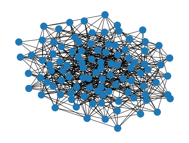
สร้างแบบจำลองปัญหา max-cut ด้วยคลาสแอปพลิเคชัน Maxcut จาก Optimization Mapper Qiskit addon มันคืน OptimizationProblem ที่มีตัวแปรไบนารีหนึ่งตัวต่อโหนด โดยมีฟังก์ชันวัตถุประสงค์คือค่า cut ที่ต้องทำให้สูงสุด ในบทแนะนำ QAOA ปัญหานี้ถูกแปลงเป็น QUBO และแปลเป็นแฮมิลโทเนียนต้นทุนที่มีหนึ่งคิวบิตต่อตัวแปร PCE กลับเข้ารหัสตัวแปรไบนารีแต่ละตัวลงในเครื่องหมายของค่าคาดหมาย Pauli ดังนั้นที่นี่ปัญหากำหนดและประเมินฟังก์ชันวัตถุประสงค์ และการเข้ารหัสลงคิวบิตตามมาด้านล่าง

maxcut = Maxcut(graph)
maxcut_problem = maxcut.to_optimization_problem()
evaluate_cut = make_cut_evaluator(maxcut_problem)

print(f"Binary variables: {maxcut_problem.get_num_vars()}")
print(
    "Quadratic terms (one per edge):",
    len(maxcut_problem.objective.quadratic.to_dict()),
)

Binary variables: 100
Quadratic terms (one per edge): 508

nx_graph = nx.Graph()
nx_graph.add_nodes_from(range(num_nodes))

for edge in graph.edge_list():
    nx_graph.add_edge(edge[0], edge[1])

curr_cut_size, partition = nx.approximation.one_exchange(nx_graph, seed=1)
print(f"Initial cut size: {curr_cut_size}")

Initial cut size: 345

เราเข้ารหัสกราฟที่มี 100 โหนดลงในความสัมพันธ์ Pauli-matrix แบบสองวัตถุบน 9 Qubit (ดูคำอธิบายด้านล่าง) กราฟถูกแทนเป็น correlation matrix โดยแต่ละโหนดถูกเข้ารหัสด้วย Pauli string เครื่องหมายของค่าคาดหวังของ Pauli string แสดงถึงพาร์ติชันของโหนด ตัวอย่างเช่น โหนด 0 ถูกเข้ารหัสด้วย Pauli string $\prod_0 = I_{8} \otimes ... I_2 \otimes X_1 \otimes X_0$ เครื่องหมายของค่าคาดหวังของ Pauli string นี้แสดงถึงพาร์ติชันของโหนด 0 เรานิยาม Pauli-correlation encoding (PCE) เทียบกับ $\prod$ เป็น

$x_i \coloneqq \textit{sgn}(\langle\prod_i \rangle),$

โดยที่ $x_i$ คือพาร์ติชันของโหนด $i$ และ $\langle \prod_i \rangle \coloneqq \langle \psi |\prod_i| \psi \rangle$ คือค่าคาดหวังของ Pauli string ที่เข้ารหัสโหนด $i$ บน quantum state $|\psi \rangle$ ตอนนี้ มาเข้ารหัสกราฟลงใน Hamiltonian โดยใช้ PCE กัน เราแบ่งโหนดออกเป็นสามเซต คือ $S_1$ , $S_2$ และ $S_3$ จากนั้น เราเข้ารหัสโหนดในแต่ละเซตโดยใช้ Pauli string ที่มี $X$ , $Y$ และ $Z$ ตามลำดับ เราจำเป็นต้องหาความสัมพันธ์ระหว่างจำนวนโหนดและจำนวน Qubit ที่ต้องการในการเข้ารหัสโหนดทั้งหมด การใช้ permutation ที่เป็นไปได้ทั้งหมดสำหรับการเข้ารหัสจะได้:

m=3\binom{n}{k}.

ในตัวอย่างนี้เราพิจารณา $k=2$ ดังนั้น

m = \frac{3}{2} n(n-1).

ด้วยเหตุนี้ จำนวน Qubit $n$ ที่ต้องการในการแสดงจำนวนโหนด $m$ ที่กำหนดจึงอ่านได้เป็น:

n = \left\lceil \frac{1 + \sqrt{1 + \tfrac{8}{3}m}}{2} \right\rceil.

หมายเหตุ: สัญลักษณ์ $\lceil \cdot \rceil$ แทนฟังก์ชัน ceiling ซึ่งปัดจำนวนจริงใด ๆ ขึ้นไปยังจำนวนเต็มถัดไป เพื่อให้แน่ใจว่าจำนวน Qubit เป็นจำนวนเต็ม

num_qubits = int(np.ceil((1 + np.sqrt(1 + (8 / 3) * num_nodes)) / 2))

list_size = num_nodes // 3
node_x = [i for i in range(list_size)]
node_y = [i for i in range(list_size, 2 * list_size)]
node_z = [i for i in range(2 * list_size, num_nodes)]

print(f"Number of qubits: {num_qubits}")
print("List 1:", node_x)
print("List 2:", node_y)
print("List 3:", node_z)

Number of qubits: 9
List 1: [0, 1, 2, 3, 4, 5, 6, 7, 8, 9, 10, 11, 12, 13, 14, 15, 16, 17, 18, 19, 20, 21, 22, 23, 24, 25, 26, 27, 28, 29, 30, 31, 32]
List 2: [33, 34, 35, 36, 37, 38, 39, 40, 41, 42, 43, 44, 45, 46, 47, 48, 49, 50, 51, 52, 53, 54, 55, 56, 57, 58, 59, 60, 61, 62, 63, 64, 65]
List 3: [66, 67, 68, 69, 70, 71, 72, 73, 74, 75, 76, 77, 78, 79, 80, 81, 82, 83, 84, 85, 86, 87, 88, 89, 90, 91, 92, 93, 94, 95, 96, 97, 98, 99]

def build_pauli_correlation_encoding(pauli, node_list, n, k=2):
    pauli_correlation_encoding = []
    for idx, c in enumerate(combinations(range(n), k)):
        if idx >= len(node_list):
            break
        paulis = ["I"] * n
        paulis[c[0]], paulis[c[1]] = pauli, pauli
        pauli_correlation_encoding.append(("".join(paulis)[::-1], 1))

    hamiltonian = []
    for pauli, weight in pauli_correlation_encoding:
        hamiltonian.append(SparsePauliOp.from_list([(pauli, weight)]))

    return hamiltonian

pauli_correlation_encoding_x = build_pauli_correlation_encoding(
    "X", node_x, num_qubits
)
pauli_correlation_encoding_y = build_pauli_correlation_encoding(
    "Y", node_y, num_qubits
)
pauli_correlation_encoding_z = build_pauli_correlation_encoding(
    "Z", node_z, num_qubits
)

ขั้นตอนที่ 2: ปรับแต่งปัญหาสำหรับการรันบนฮาร์ดแวร์ควอนตัม

Quantum Circuit

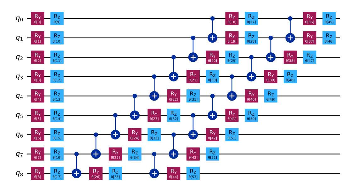
ที่นี่ state $|\psi \rangle$ ถูก parameterize ด้วย $\mathbf{\theta}$ และเราปรับแต่ง parameter $\mathbf{\theta}$ เหล่านี้โดยใช้แนวทาง variational บทแนะนำนี้ใช้ ansatz efficient_su2 สำหรับอัลกอริทึม variational ของเราเนื่องจากความสามารถในการแสดงออกและความง่ายในการนำไปใช้ นอกจากนี้เรายังใช้ฟังก์ชันการสูญเสียแบบ relaxed ซึ่งจะแนะนำในภายหลังในบทแนะนำนี้ ด้วยเหตุนี้ เราจึงสามารถจัดการกับปัญหาขนาดใหญ่ได้ด้วย Qubit จำนวนน้อยกว่าและความลึกของ Circuit ที่ตื้นกว่า

# Build the quantum circuit
qc = efficient_su2(num_qubits, su2_gates=["ry", "rz"], reps=2)
qc.draw("mpl")

Output of the previous code cell

# Optimize the circuit

pm = generate_preset_pass_manager(optimization_level=3, backend=backend)
qc = pm.run(qc)

ฟังก์ชันการสูญเสีย

สำหรับฟังก์ชันการสูญเสีย $\mathcal{L}$ เราใช้การ relax ของฟังก์ชันวัตถุประสงค์ max-cut ตามที่อธิบายใน [1] ซึ่งนิยามเป็น $\mathcal{V}(\mathbf{x}) \coloneqq \sum_{(i, j) \in E} W_{i, j}(1-x_i x_j)$ โดยที่ $W_{i, j}$ แทนน้ำหนักของเส้นเชื่อม $(i, j)$ และ $x_i$ แทนพาร์ติชันของโหนด $i$ ฟังก์ชันการสูญเสีย $\mathcal{L}$ ถูกกำหนดโดย:

$\mathcal{L}\coloneqq \sum_{(i, j) \in E} W_{i, j} \text{tanh} (\alpha \langle\prod_i \rangle) \text{tanh} (\alpha \langle\prod_j \rangle) + \mathcal{L}^{(\text{reg})}$ ,

โดยที่ฟังก์ชันวัตถุประสงค์ max-cut ถูกแทนที่ด้วย hyperbolic tangent แบบ smooth ของค่าคาดหวังของ Pauli string ที่เข้ารหัสโหนด พจน์การทำให้เป็นระเบียบ $\mathcal{L}^{(\text{reg})}$ และปัจจัยการปรับขนาด $\alpha$ ซึ่งแปรผันตามจำนวน Qubit ถูกนำเข้ามาเพื่อปรับปรุงประสิทธิภาพของตัวแก้ปัญหา

พจน์การทำให้เป็นระเบียบถูกนิยามเป็น:

$\mathcal{L}^{(\text{reg})}$ ถูกนิยามเป็น $\mathcal{L}^{(\text{reg})} \coloneqq \beta \nu \lbrack \frac{1}{m} \sum_{i \in V} \text{tanh} (\alpha \langle\prod_i \rangle)^2 \rbrack ^2$

โดยที่ $\beta=1/2$ , $\nu = |E|/2 + (m -1) /4$ , $|E|$ คือจำนวนเส้นเชื่อม และ $m$ คือจำนวนโหนดในกราฟ

def loss_func_estimator(x, ansatz, hamiltonian, estimator, graph):
    """
    Calculates the specified loss function for the given ansatz, Hamiltonian,
    and graph.

    The expectation values of each Pauli string in the Hamiltonian are first
    obtained by running the ansatz on the quantum backend. These
    expectation values are then passed through the nonlinear function
    tanh(alpha * prod_i). The loss function is
    subsequently computed from these transformed values.
    """
    job = estimator.run(
        [
            (ansatz, hamiltonian[0], x),
            (ansatz, hamiltonian[1], x),
            (ansatz, hamiltonian[2], x),
        ]
    )
    result = job.result()

    # calculate the loss function
    node_exp_map = {}
    idx = 0
    for r in result:
        for ev in r.data.evs:
            node_exp_map[idx] = ev
            idx += 1

    loss = 0
    alpha = num_qubits
    for edge0, edge1 in graph.edge_list():
        loss += np.tanh(alpha * node_exp_map[edge0]) * np.tanh(
            alpha * node_exp_map[edge1]
        )

    regulation_term = 0
    for i in range(len(graph.nodes())):
        regulation_term += np.tanh(alpha * node_exp_map[i]) ** 2
    regulation_term = regulation_term / len(graph.nodes())
    regulation_term = regulation_term**2
    beta = 1 / 2
    v = len(graph.edges()) / 2 + (len(graph.nodes()) - 1) / 4
    regulation_term = beta * v * regulation_term

    loss = loss + regulation_term

    global experiment_result
    print(f"Iter {len(experiment_result)}: {loss}")
    experiment_result.append({"loss": loss, "exp_map": node_exp_map})
    return loss

ขั้นตอนที่ 3: รันโดยใช้ Qiskit primitives

ในบทแนะนำนี้ เราตั้ง max_iter=50 ในลูปการปรับค่าเพื่อวัตถุประสงค์การสาธิต ถ้าเพิ่มจำนวนรอบการวนซ้ำ เราคาดว่าจะได้ผลลัพธ์ที่ดีขึ้น

pce = []
pce.append(
    [op.apply_layout(qc.layout) for op in pauli_correlation_encoding_x]
)
pce.append(
    [op.apply_layout(qc.layout) for op in pauli_correlation_encoding_y]
)
pce.append(
    [op.apply_layout(qc.layout) for op in pauli_correlation_encoding_z]
)

max_iter = 50
counter = {"i": 0}
last_x = {"value": None}
last_fun = {"value": None}

with Session(backend=backend) as session:
    estimator = Estimator(mode=session)

    experiment_result = []

    def loss_func(x):
        last_x["value"] = x.copy()
        if counter["i"] + 1 > max_iter:
            return last_fun["value"]
        counter["i"] += 1
        val = loss_func_estimator(
            x, qc, [pce[0], pce[1], pce[2]], estimator, graph
        )
        last_fun["value"] = val
        return val

    np.random.seed(seed)
    initial_params = np.random.rand(qc.num_parameters)

    result = minimize(
        loss_func, initial_params, method="COBYLA", options={"rhobeg": 1.0}
    )

    if counter["i"] >= max_iter:
        result = OptimizeResult(
            message=f"Return from COBYLA because the objective function "
            f"has been evaluated {max_iter} times.",
            success=False,
            status=3,
            fun=last_fun["value"],
            x=last_x["value"],
            nfev=counter["i"],
        )

print(result)

Iter 0: 152.06331779109445

Iter 1: 126.93132569244693

Iter 2: 55.00651109478942

Iter 3: 33.21667439735082

Iter 4: 19.167189700765054

Iter 5: 30.426875553389127

Iter 6: 13.906354614925815

Iter 7: 27.668686100172614

Iter 8: 28.194600411380772

Iter 9: 24.899677141564936

Iter 10: 22.10858041608358

Iter 11: 8.096210209030176

Iter 12: 8.761240650022913

Iter 13: 9.43332962472133

Iter 14: 7.559669820210062

Iter 15: 13.023860357384214

Iter 16: 11.953653163007987

Iter 17: 10.434221292269214

Iter 18: 4.871246922225549

Iter 19: 10.303826533395856

Iter 20: 16.40225843511339

Iter 21: 10.852469442638652

Iter 22: 9.314666066331633

Iter 23: 6.082358010011717

Iter 24: 10.982893700414476

Iter 25: 4.575556036893407

Iter 26: 6.844995727798197

Iter 27: 8.695229718011293

Iter 28: 3.730227705075576

Iter 29: 4.285479467758721

Iter 30: 4.219714169314187

Iter 31: 0.21125608131726548

Iter 32: 4.22820465672552

Iter 33: 13.67513152473414

Iter 34: 10.388838701884863

Iter 35: -0.5400153834163355

Iter 36: 5.310281742761159

Iter 37: -0.5430772019249082

Iter 38: -4.47820293096989

Iter 39: -3.4832056790567467

Iter 40: -0.5087341672330172

Iter 41: -2.488777859669888

Iter 42: 0.34945469121089356

Iter 43: -0.8544299675507805

Iter 44: -3.5902371208579344

Iter 45: 2.6609573847203216

Iter 46: -4.336467834641085

Iter 47: 0.10158504073828034

Iter 48: -1.3506458813942084

Iter 49: -2.1794894170194192

message: Return from COBYLA because the objective function has been evaluated 50 times.
 success: False
  status: 3
     fun: -2.1794894170194192
       x: [ 1.375e+00  1.951e+00 ...  9.395e-01  8.948e-01]
    nfev: 50

ขั้นตอนที่ 4: ประมวลผลหลังและส่งคืนผลลัพธ์ในรูปแบบคลาสสิกที่ต้องการ

พาร์ติชันของโหนดถูกกำหนดโดยประเมินเครื่องหมายของค่าคาดหมายของสตริง Pauli ที่เข้ารหัสโหนด ค่าคาดหมายที่ไม่เป็นลบกำหนดค่า 1 ให้โหนด และค่าคาดหมายที่เป็นลบกำหนด 0 จากนั้นเมธอด interpret ของ Maxcut ถอดรหัสการกำหนดนี้เป็นสองเซตของโหนด

# Decode the node assignment from the iteration with the lowest loss.
# If the expectation value is non-negative, the node is assigned 1,
# otherwise it is assigned 0.
def get_bits(experiment_result):
    best_index = min(
        range(len(experiment_result)),
        key=lambda i: experiment_result[i]["loss"],
    )
    exp_map = experiment_result[best_index]["exp_map"]
    bits = [1 if exp_map[i] >= 0 else 0 for i in range(len(exp_map))]
    return bits, best_index

cur_bits, best_index = get_bits(experiment_result)
partition = maxcut.interpret(np.array(cur_bits))
print("Partition 0:", partition[0])
print("Partition 1:", partition[1])

Partition 0: [0, 1, 3, 5, 6, 7, 9, 11, 12, 14, 15, 17, 22, 24, 25, 28, 31, 32, 33, 35, 37, 38, 39, 40, 41, 43, 49, 53, 54, 56, 59, 61, 63, 65, 67, 68, 69, 77, 78, 79, 80, 88, 92, 93, 94, 95]
Partition 1: [2, 4, 8, 10, 13, 16, 18, 19, 20, 21, 23, 26, 27, 29, 30, 34, 36, 42, 44, 45, 46, 47, 48, 50, 51, 52, 55, 57, 58, 60, 62, 64, 66, 70, 71, 72, 73, 74, 75, 76, 81, 82, 83, 84, 85, 86, 87, 89, 90, 91, 96, 97, 98, 99]

เราคำนวณขนาด cut ของปัญหา max-cut ได้โดยประเมินฟังก์ชันวัตถุประสงค์ของ OptimizationProblem บนการกำหนดนี้

cut_size = evaluate_cut(cur_bits)
print(f"Cut size: {cut_size}")

Cut size: 278

เมื่อการเทรนเสร็จสิ้น เราทำการค้นหาแบบ single-bit swap หนึ่งรอบเพื่อปรับปรุงผลลัพธ์ในฐานะขั้นตอนการประมวลผลหลัง (post-processing) แบบคลาสสิก ในกระบวนการนี้ เราสลับพาร์ติชันของโหนดสองโหนดและประเมินขนาด cut ถ้าขนาด cut ดีขึ้น เราจะเก็บการสลับนั้นไว้ เราทำซ้ำกระบวนการนี้สำหรับคู่โหนดที่เชื่อมต่อกันด้วย edge ทุกคู่ที่เป็นไปได้

# Swap the partitions and calculate the cut size

def swap_partitions(graph, cur_bits, evaluate_cut):
    best_cut = 0
    best_bits = []
    for edge0, edge1 in graph.edge_list():
        swapped_bits = cur_bits.copy()
        swapped_bits[edge0], swapped_bits[edge1] = (
            swapped_bits[edge1],
            swapped_bits[edge0],
        )
        cut_size = evaluate_cut(swapped_bits)
        if best_cut < cut_size:
            best_cut = cut_size
            best_bits = swapped_bits
    return best_cut, best_bits

best_cut, best_bits = swap_partitions(graph, cur_bits, evaluate_cut)
print(best_cut, best_bits)

287 [0, 0, 1, 0, 1, 0, 0, 0, 1, 0, 1, 0, 0, 1, 0, 0, 1, 0, 1, 1, 1, 1, 0, 1, 0, 0, 1, 1, 0, 1, 1, 0, 0, 0, 1, 1, 0, 0, 0, 0, 0, 0, 1, 0, 1, 1, 1, 1, 1, 0, 1, 1, 1, 0, 0, 1, 0, 1, 1, 0, 1, 0, 1, 0, 1, 0, 1, 0, 0, 0, 1, 1, 1, 1, 1, 1, 1, 0, 0, 0, 0, 1, 1, 1, 1, 1, 1, 1, 0, 1, 1, 1, 0, 0, 0, 0, 1, 1, 1, 1]

ตัวอย่างบนฮาร์ดแวร์จริงขนาดใหญ่

# -------------------------Step 1-------------------------

num_nodes = 1500  # Number of nodes in graph
graph = rx.undirected_gnp_random_graph(num_nodes, 0.1, seed=seed)
nx_graph = nx.Graph()
nx_graph.add_nodes_from(range(num_nodes))
for edge in graph.edge_list():
    nx_graph.add_edge(edge[0], edge[1])

maxcut = Maxcut(graph)
maxcut_problem = maxcut.to_optimization_problem()
evaluate_cut = make_cut_evaluator(maxcut_problem)

num_qubits = int(np.ceil((1 + np.sqrt(1 + (8 / 3) * num_nodes)) / 2))

list_size = num_nodes // 3
node_x = [i for i in range(list_size)]
node_y = [i for i in range(list_size, 2 * list_size)]
node_z = [i for i in range(2 * list_size, num_nodes)]

pauli_correlation_encoding_x = build_pauli_correlation_encoding(
    "X", node_x, num_qubits
)
pauli_correlation_encoding_y = build_pauli_correlation_encoding(
    "Y", node_y, num_qubits
)
pauli_correlation_encoding_z = build_pauli_correlation_encoding(
    "Z", node_z, num_qubits
)
print(f"We are using {num_qubits} qubits")

# -------------------------Step 2-------------------------
backend = real_backend
print(f"We are using the {backend.name}")
qc = efficient_su2(num_qubits, ["ry", "rz"], reps=2)
pm = generate_preset_pass_manager(optimization_level=3, backend=backend)
qc = pm.run(qc)
# -------------------------Step 3-------------------------
pce = []
pce.append(
    [op.apply_layout(qc.layout) for op in pauli_correlation_encoding_x]
)
pce.append(
    [op.apply_layout(qc.layout) for op in pauli_correlation_encoding_y]
)
pce.append(
    [op.apply_layout(qc.layout) for op in pauli_correlation_encoding_z]
)

# Run the optimization using a session.
max_iter = 50
counter = {"i": 0}
with Session(backend=backend) as session:
    estimator = Estimator(mode=session)
    estimator.options.environment.job_tags = ["TUT_PCEFQ"]
    experiment_result = []

    def loss_func(x):
        last_x["value"] = x.copy()
        if counter["i"] + 1 > max_iter:
            return last_fun["value"]
        counter["i"] += 1
        val = loss_func_estimator(
            x, qc, [pce[0], pce[1], pce[2]], estimator, graph
        )
        last_fun["value"] = val
        return val

    np.random.seed(seed)
    initial_params = np.random.rand(qc.num_parameters)
    result = minimize(
        loss_func, initial_params, method="COBYLA", options={"rhobeg": 1.0}
    )
    if counter["i"] >= max_iter:
        result = OptimizeResult(
            message=f"Return from COBYLA because the objective function "
            f"has been evaluated {max_iter} times.",
            success=False,
            status=3,
            fun=last_fun["value"],
            x=last_x["value"],
            nfev=counter["i"],
        )
print(result)

# -------------------------Step 4-------------------------

cur_bits, best_index = get_bits(experiment_result)
cut_size = evaluate_cut(cur_bits)
print(f"Cut size: {cut_size}")

best_cut, best_bits = swap_partitions(graph, cur_bits, evaluate_cut)
# Print final solution

print(
    f"The best max-cut value achieved for a graph with {num_nodes} nodes "
    f"on {num_qubits} qubits is {best_cut}"
)
print(f"and the specific partition we obtained is {best_bits}")

We are using 33 qubits
We are using the ibm_pittsburgh

Iter 0: 62192.56098951446

Iter 1: 54325.76340818571

Iter 2: 42933.215216568526

Iter 3: 35721.92960658595

Iter 4: 35947.69927402131

Iter 5: 38563.731543582166

Iter 6: 32552.97070835923

Iter 7: 34730.314616527576

Iter 8: 27032.920190652876

Iter 9: 27126.107795624957

Iter 10: 25268.853826648774

Iter 11: 23521.1489346676

Iter 12: 21658.585394613096

Iter 13: 15154.765728388778

Iter 14: 14826.985321939152

Iter 15: 16199.811009055386

Iter 16: 14328.589985020852

Iter 17: 13542.67789354434

Iter 18: 11737.341026421902

Iter 19: 10986.431644208033

Iter 20: 9780.61657788984

Iter 21: 8555.757154943312

Iter 22: 10465.489221259657

Iter 23: 8577.158776664453

Iter 24: 8950.176436175909

Iter 25: 7395.8803219317215

Iter 26: 7228.1129297581765

Iter 27: 6881.076354027118

Iter 28: 6626.8983738084835

Iter 29: 7302.433279572058

Iter 30: 6995.735525608492

Iter 31: 6176.828001182083

Iter 32: 6299.8061884979725

Iter 33: 6498.921256598082

Iter 34: 6184.684072713035

Iter 35: 5707.720358527108

Iter 36: 5414.328928670104

Iter 37: 5771.80573980932

Iter 38: 5620.64903695431

Iter 39: 6285.735849503706

Iter 40: 5894.367571492991

Iter 41: 6079.275064349491

Iter 42: 5267.448536682269

Iter 43: 4789.7281459863325

Iter 44: 5109.106057200384

Iter 45: 5060.248865782273

Iter 46: 5064.786713246322

Iter 47: 5474.433264995371

Iter 48: 4675.6138719238015

Iter 49: 5081.660754434205

message: Return from COBYLA because the objective function has been evaluated 50 times.
 success: False
  status: 3
     fun: 5081.660754434205
       x: [ 1.375e+00  1.951e+00 ...  7.260e-01  8.971e-01]
    nfev: 50
Cut size: 55507

The best max-cut value achieved for a graph with 1500 nodes on 33 qubits is 55567
and the specific partition we obtained is [1, 0, 0, 1, 1, 1, 1, 0, 0, 1, 1, 1, 0, 1, 0, 1, 0, 0, 0, 1, 1, 0, 1, 0, 0, 1, 1, 0, 0, 1, 1, 1, 0, 0, 0, 0, 0, 1, 0, 0, 0, 1, 1, 1, 1, 0, 0, 0, 0, 1, 0, 0, 0, 0, 1, 1, 1, 0, 1, 1, 1, 0, 1, 0, 0, 0, 0, 0, 0, 1, 0, 1, 1, 0, 0, 1, 1, 1, 1, 0, 1, 0, 1, 1, 0, 1, 1, 0, 0, 0, 1, 1, 1, 0, 1, 1, 0, 0, 1, 0, 0, 0, 1, 1, 1, 1, 1, 1, 1, 1, 0, 0, 0, 1, 1, 1, 1, 1, 1, 0, 0, 0, 1, 1, 0, 1, 0, 1, 0, 1, 0, 1, 1, 1, 0, 0, 0, 0, 1, 0, 0, 0, 0, 0, 0, 0, 1, 0, 1, 1, 1, 0, 1, 0, 1, 0, 1, 0, 0, 0, 1, 0, 0, 0, 0, 1, 0, 0, 1, 1, 1, 1, 1, 1, 1, 1, 1, 1, 1, 0, 1, 0, 0, 0, 0, 0, 0, 0, 1, 0, 1, 1, 1, 1, 1, 1, 1, 1, 1, 1, 0, 1, 1, 0, 0, 0, 0, 0, 0, 0, 0, 0, 0, 0, 1, 1, 0, 0, 0, 0, 0, 1, 0, 0, 0, 0, 0, 1, 0, 1, 0, 0, 0, 0, 1, 0, 1, 1, 1, 1, 1, 0, 1, 1, 0, 0, 1, 1, 1, 0, 1, 1, 1, 1, 0, 1, 0, 1, 1, 0, 1, 1, 1, 0, 0, 0, 0, 1, 1, 1, 1, 0, 0, 1, 1, 1, 1, 1, 1, 1, 1, 0, 1, 0, 0, 0, 0, 1, 0, 0, 0, 1, 1, 1, 0, 1, 1, 0, 1, 1, 1, 1, 1, 1, 1, 1, 1, 0, 0, 1, 1, 0, 0, 0, 1, 0, 1, 0, 0, 1, 0, 1, 1, 1, 0, 0, 1, 1, 1, 1, 1, 0, 1, 0, 0, 1, 0, 1, 1, 1, 1, 1, 0, 1, 1, 1, 0, 1, 1, 1, 1, 0, 0, 1, 1, 1, 1, 1, 1, 1, 0, 1, 0, 0, 1, 0, 1, 0, 0, 0, 0, 0, 1, 0, 0, 1, 0, 0, 1, 1, 1, 0, 1, 1, 1, 1, 0, 1, 1, 1, 1, 0, 1, 1, 0, 1, 1, 1, 1, 1, 1, 1, 1, 1, 0, 0, 1, 1, 1, 0, 0, 0, 1, 1, 0, 1, 0, 1, 0, 1, 0, 1, 0, 1, 0, 0, 0, 0, 1, 1, 1, 1, 1, 1, 1, 1, 0, 1, 0, 0, 0, 1, 0, 0, 0, 1, 0, 0, 1, 1, 1, 0, 0, 0, 0, 1, 0, 1, 0, 1, 1, 1, 1, 1, 0, 1, 0, 1, 1, 0, 1, 1, 1, 1, 0, 1, 0, 1, 0, 1, 1, 1, 0, 1, 1, 1, 1, 1, 1, 0, 1, 1, 1, 1, 0, 1, 1, 1, 1, 0, 0, 1, 1, 1, 0, 0, 1, 0, 1, 1, 0, 1, 1, 1, 1, 0, 0, 1, 0, 1, 0, 1, 1, 1, 1, 0, 1, 0, 0, 1, 0, 1, 1, 1, 0, 0, 0, 1, 1, 0, 0, 1, 0, 1, 1, 1, 1, 1, 0, 1, 0, 0, 0, 0, 1, 0, 1, 0, 1, 0, 0, 0, 1, 0, 0, 0, 0, 1, 0, 0, 0, 1, 0, 1, 1, 1, 0, 1, 1, 1, 1, 0, 0, 0, 0, 0, 1, 0, 1, 0, 1, 1, 1, 1, 0, 0, 1, 1, 0, 0, 0, 1, 1, 1, 1, 1, 1, 0, 0, 1, 0, 0, 1, 0, 0, 0, 0, 0, 0, 1, 0, 1, 1, 1, 1, 1, 0, 1, 0, 1, 1, 1, 1, 0, 1, 0, 0, 1, 1, 1, 1, 0, 1, 1, 1, 1, 0, 1, 1, 0, 1, 0, 0, 1, 0, 1, 1, 1, 0, 0, 0, 1, 1, 0, 1, 1, 1, 1, 1, 1, 1, 1, 1, 1, 1, 1, 0, 0, 0, 1, 1, 0, 0, 0, 1, 1, 1, 1, 1, 1, 0, 0, 1, 0, 1, 1, 0, 0, 0, 0, 0, 0, 0, 0, 1, 0, 1, 0, 1, 0, 0, 0, 1, 1, 0, 0, 0, 0, 1, 1, 1, 1, 1, 0, 1, 1, 0, 1, 0, 1, 1, 1, 0, 1, 1, 1, 0, 1, 0, 1, 1, 1, 1, 0, 1, 1, 1, 1, 1, 1, 1, 1, 0, 0, 0, 0, 0, 0, 0, 1, 0, 0, 0, 0, 0, 0, 1, 0, 1, 0, 1, 0, 0, 0, 1, 0, 1, 0, 1, 0, 1, 0, 0, 0, 1, 0, 1, 1, 1, 0, 1, 1, 0, 0, 1, 1, 0, 1, 1, 0, 1, 1, 1, 1, 1, 1, 0, 0, 1, 1, 0, 1, 1, 1, 1, 1, 1, 0, 0, 1, 1, 1, 0, 0, 0, 0, 0, 1, 1, 1, 0, 1, 1, 0, 1, 0, 1, 0, 0, 1, 1, 1, 1, 1, 1, 0, 0, 0, 1, 1, 0, 0, 1, 0, 1, 1, 0, 0, 0, 1, 0, 0, 0, 0, 1, 1, 0, 1, 0, 1, 0, 1, 0, 0, 1, 0, 1, 1, 1, 0, 1, 0, 1, 1, 1, 1, 1, 0, 1, 0, 1, 0, 0, 1, 0, 1, 0, 1, 0, 1, 0, 0, 0, 1, 0, 0, 1, 0, 0, 1, 0, 1, 0, 0, 0, 0, 1, 1, 0, 1, 0, 1, 0, 0, 1, 1, 1, 0, 1, 1, 1, 1, 0, 1, 0, 1, 0, 0, 1, 0, 0, 1, 0, 1, 1, 0, 0, 1, 0, 1, 0, 1, 0, 1, 1, 1, 0, 1, 0, 0, 1, 0, 0, 0, 0, 0, 1, 1, 1, 0, 1, 1, 0, 1, 0, 1, 0, 1, 1, 1, 0, 0, 0, 1, 1, 1, 1, 1, 1, 1, 1, 0, 1, 1, 1, 1, 1, 0, 1, 0, 0, 0, 0, 1, 1, 1, 1, 1, 1, 1, 1, 0, 1, 0, 1, 1, 1, 1, 0, 1, 1, 1, 1, 0, 1, 1, 1, 1, 1, 1, 1, 1, 0, 1, 0, 0, 0, 1, 0, 1, 0, 0, 1, 1, 1, 1, 0, 0, 1, 0, 0, 0, 1, 0, 0, 1, 0, 0, 0, 1, 1, 0, 1, 1, 0, 0, 0, 1, 0, 0, 0, 0, 0, 1, 0, 1, 0, 1, 0, 0, 1, 0, 0, 0, 0, 1, 0, 0, 0, 0, 0, 0, 0, 0, 0, 0, 1, 0, 1, 0, 0, 0, 0, 1, 0, 0, 0, 1, 0, 1, 0, 1, 0, 0, 0, 0, 0, 0, 0, 1, 0, 0, 1, 1, 0, 1, 1, 1, 0, 1, 0, 0, 0, 1, 1, 1, 1, 1, 1, 1, 1, 1, 0, 1, 1, 1, 0, 0, 1, 0, 1, 0, 1, 0, 1, 1, 0, 0, 0, 1, 1, 1, 1, 1, 1, 1, 1, 1, 1, 0, 1, 1, 1, 1, 0, 1, 0, 0, 1, 1, 1, 1, 0, 0, 0, 1, 1, 1, 1, 1, 1, 1, 1, 1, 1, 0, 1, 1, 1, 1, 1, 1, 0, 0, 1, 0, 0, 0, 1, 0, 1, 0, 0, 0, 0, 0, 0, 1, 0, 0, 0, 0, 0, 0, 1, 0, 0, 0, 0, 1, 0, 0, 0, 0, 1, 1, 0, 1, 1, 1, 1, 1, 1, 1, 0, 1, 1, 1, 1, 1, 1, 0, 1, 1, 1, 0, 0, 0, 1, 1, 1, 0, 0, 1, 1, 1, 0, 1, 1, 1, 0, 1, 1, 1, 1, 0, 0, 0, 1, 0, 1, 1, 0, 1, 1, 1, 1, 1, 1, 1, 1, 1, 1, 1, 0, 1, 0, 1, 0, 0, 0, 1, 1, 1, 1, 0, 0, 0, 1, 0, 0, 0, 0, 0, 1, 0, 1, 0, 1, 1, 1, 0, 0, 1, 0, 1, 1, 1, 0, 0, 1, 0, 0, 0, 0, 1, 0, 1, 1, 0, 0, 1, 0, 0, 0, 0, 0, 0, 0, 0, 0, 0, 0, 0, 0, 0, 0, 1, 0, 0, 1, 0, 0, 0, 0, 0, 0, 1, 0, 0, 0, 0, 0, 0, 0, 1, 1, 1, 0, 1, 1, 0, 1, 0, 1, 1, 1, 1, 1, 1, 1, 0, 1, 1, 0, 1, 1, 1, 1, 1, 1, 1, 1, 1, 1, 0, 1, 0, 1, 1, 0, 1, 0, 1, 1, 0, 1, 0, 1, 1, 1, 1, 0, 1, 1, 0, 0, 0, 0, 1, 0, 1, 0, 0, 0, 0, 0, 1, 1, 0, 1, 0, 0, 1, 1, 1, 0, 0, 1, 0, 1, 0, 1, 1, 0, 1, 0, 1, 1, 1, 1, 1, 0, 1, 1, 1, 1, 1, 1, 1, 1, 1, 0, 1, 1, 1, 0, 1, 1, 1, 1, 1, 1, 1, 1, 1, 1, 1, 1, 1, 1, 0, 1, 1, 0, 1, 1, 1, 1, 1]

ขั้นตอนถัดไป

Recommendations

หากคุณพบว่างานนี้น่าสนใจ คุณอาจสนใจเนื้อหาต่อไปนี้:

References

[1] Sciorilli, M., Borges, L., Patti, T. L., García-Martín, D., Camilo, G., Anandkumar, A., & Aolita, L. (2024). Towards large-scale quantum optimization solvers with few qubits. arXiv preprint arXiv:2401.09421.

แบบสำรวจบทเรียน

กรุณาทำแบบสำรวจสั้น ๆ นี้เพื่อให้ข้อเสนอแนะเกี่ยวกับบทแนะนำนี้ ความคิดเห็นของคุณจะช่วยให้เราปรับปรุงเนื้อหาและประสบการณ์การใช้งาน

หมายเหตุ: แบบสำรวจนี้จัดทำโดย IBM Quantum และครอบคลุม เนื้อหาบทเรียน (เขียนโดย IBM) doQumentation เป็นผู้ให้บริการเว็บไซต์ การแปล และการรันโค้ด — สำหรับความคิดเห็นเกี่ยวกับสิ่งเหล่านั้น โปรดเปิด GitHub issue.

ผลลัพธ์การเรียนรู้​

ข้อกำหนดเบื้องต้น​

พื้นหลัง​

ภาพรวม​

ข้อกำหนด​

การตั้งค่า​

ตัวอย่างด้วย Simulator ขนาดเล็ก​

ขั้นตอนที่ 1: แมปอินพุตคลาสสิกไปยังปัญหาเชิงควอนตัม​

ปัญหา max-cut​

กราฟ → ปัญหาการหาค่าเหมาะที่สุด​

ขั้นตอนที่ 2: ปรับแต่งปัญหาสำหรับการรันบนฮาร์ดแวร์ควอนตัม​

Quantum Circuit​

ฟังก์ชันการสูญเสีย​

ขั้นตอนที่ 3: รันโดยใช้ Qiskit primitives​

ขั้นตอนที่ 4: ประมวลผลหลังและส่งคืนผลลัพธ์ในรูปแบบคลาสสิกที่ต้องการ​