อัลกอริทึมการหาค่าเหมาะสมแบบควอนตัมโดยประมาณ

ประมาณเวลาการใช้งาน: 22 นาทีบนโปรเซสเซอร์ Heron r3 (หมายเหตุ: นี่เป็นเพียงการประมาณเท่านั้น เวลาจริงอาจแตกต่างกัน)

ผลลัพธ์การเรียนรู้

หลังจากเรียนจบบทแนะนำนี้ คุณจะเข้าใจข้อมูลต่อไปนี้:

• วิธีแมปปัญหาการหาค่าเหมาะสมเชิงคอมบินาทอริกแบบคลาสสิก (max-cut) ไปยัง Hamiltonian ควอนตัม
• วิธีนำไปใช้และรันอัลกอริทึมการหาค่าเหมาะสมแบบควอนตัมโดยประมาณ (QAOA) โดยใช้ session ของ Qiskit Runtime
• วิธีขยายขนาด workflow ของ QAOA จากตัวอย่างเล็ก ๆ บน simulator ไปสู่การรันบนฮาร์ดแวร์ในระดับ utility scale

ข้อกำหนดเบื้องต้น

แนะนำให้คุณทำความคุ้นเคยกับหัวข้อเหล่านี้:

• Basics of quantum circuits
• Variational algorithms
• QAOA in depth — สำหรับการอธิบายอย่างครอบคลุมเกี่ยวกับอัลกอริทึม QAOA และการนำไปใช้ในระดับ utility scale

พื้นหลัง

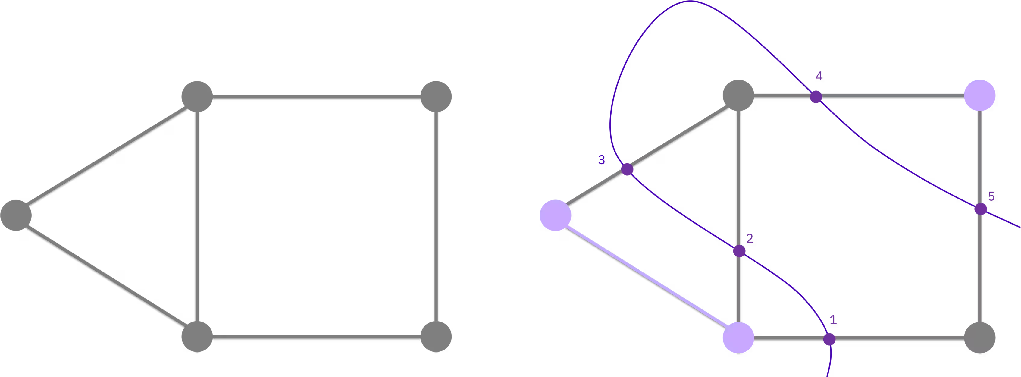
อัลกอริทึมการหาค่าเหมาะสมแบบควอนตัมโดยประมาณ (Quantum Approximate Optimization Algorithm หรือ QAOA) เป็นวิธีการแบบไฮบริดควอนตัม-คลาสสิกแบบวนซ้ำสำหรับการแก้ปัญหาการหาค่าเหมาะสมเชิงคอมบินาทอริก ในบทแนะนำนี้คุณจะใช้ QAOA เพื่อแก้ปัญหา maximum-cut (max-cut) — ปัญหาการหาค่าเหมาะสมที่เป็น NP-hard ซึ่งมีการประยุกต์ใช้ในด้านการจัดกลุ่ม วิทยาศาสตร์เครือข่าย และฟิสิกส์สถิติ เมื่อมีกราฟของโหนดที่เชื่อมต่อกันด้วยเส้นเชื่อม เป้าหมายคือการแบ่งโหนดออกเป็นสองกลุ่มเพื่อให้จำนวนเส้นเชื่อมที่ข้ามการแบ่งนี้มีค่าสูงสุด

จากการหาค่าเหมาะสมแบบคลาสสิกไปสู่ Circuit ควอนตัม

Max-cut สามารถแสดงเป็นปัญหาการหาค่าเหมาะสมไบนารีแบบคลาสสิกได้ แต่ละโหนดจะถูกกำหนดตัวแปรไบนารี $x_i \in \{0, 1\}$ ที่บ่งบอกว่ามันอยู่ในกลุ่มใด เป้าหมายคือการหาค่าสูงสุดของจำนวนเส้นเชื่อมที่จุดปลายทั้งสองอยู่คนละกลุ่ม:

$$\max_{x \in \{0,1\}^n} \sum_{(i,j)} x_i + x_j - 2x_ix_j.$$

ซึ่งเทียบเท่ากับปัญหา Quadratic Unconstrained Binary Optimization (QUBO) ในรูปแบบ $\min_x\, x^T Q x$ ผ่านการแทนตัวแปรแบบมาตรฐาน ($x_i \to (1 - Z_i)/2$) ปัญหา QUBO สามารถเขียนใหม่เป็น cost Hamiltonian ที่ ground state เข้ารหัสคำตอบที่เหมาะสมที่สุด โดยทั่วไป Hamiltonian นี้มีทั้งพจน์กำลังสองและพจน์เชิงเส้น:

$$H_C = \sum_{ij} Q_{ij} \, Z_i Z_j + \sum_i b_i \, Z_i.$$

สำหรับปัญหา max-cut แบบไม่มีน้ำหนักที่พิจารณาในที่นี้ สัมประสิทธิ์เชิงเส้นจะหายไป ($b_i = 0$) และ $Q_{ij} = 1$ สำหรับแต่ละเส้นเชื่อม ทำให้เหลือรูปแบบที่ง่ายกว่า $H_C = \sum_{(i,j) \in E} Z_i Z_j$ ซึ่งคุณจะสร้างในโค้ดด้านล่าง รูปแบบทั่วไปข้างต้นคือสิ่งที่คุณจะต้องใช้เพื่อปรับ workflow นี้ให้เข้ากับกราฟแบบมีน้ำหนักหรือปัญหาอื่น ๆ ที่แสดงในรูป QUBO ได้

QAOA ทำงานอย่างไร

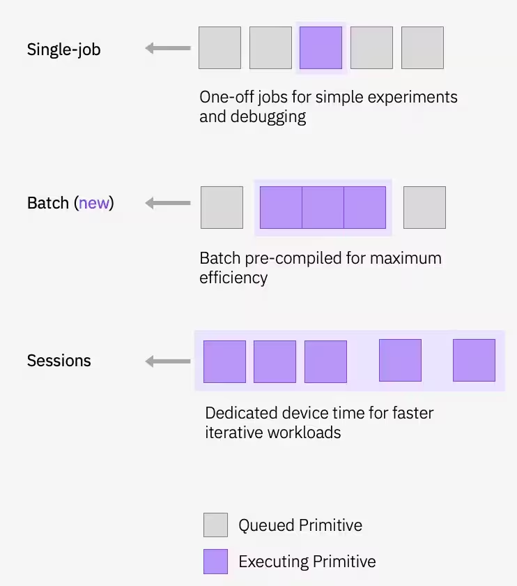
QAOA เตรียมคำตอบที่เป็นตัวเลือกโดยการใช้ชั้นสลับกันของ operator สองตัวกับสถานะ superposition เริ่มต้น $H^{\otimes n}|0\rangle$: cost operator $e^{-i\gamma_k H_C}$ และ mixer operator $e^{-i\beta_k H_m}$ มุม $\gamma_k$ และ $\beta_k$ จะถูกหาค่าเหมาะสมในลูปป้อนกลับแบบคลาสสิก คอมพิวเตอร์ควอนตัมจะประเมินฟังก์ชันต้นทุน และตัวหาค่าเหมาะสมแบบคลาสสิกจะอัปเดตพารามิเตอร์จนกว่าจะลู่เข้า ลูปวนซ้ำนี้รันภายใน session ของ Qiskit Runtime ซึ่งทำให้อุปกรณ์ควอนตัมถูกจองไว้ตลอดทุกการวนซ้ำเพื่อลด latency

สำหรับการอธิบายทฤษฎี QAOA เชิงลึก รวมถึงการอนุพันธ์เต็มจาก QUBO ไปยัง Hamiltonian ดูที่ โมดูลหลักสูตร QAOA

ในบทแนะนำนี้คุณจะแก้ปัญหา max-cut บนกราฟขนาดเล็กที่มีห้าโหนดก่อน แล้วจึงขยาย workflow เดียวกันไปสู่ปัญหาระดับ utility scale ที่มี 100 โหนดบนฮาร์ดแวร์จริง หมายเหตุเกี่ยวกับการเข้าถึงแพลน: บทแนะนำนี้ใช้ sessions ของ Qiskit Runtime ซึ่งใช้ได้เฉพาะกับ Premium Plan เท่านั้น หากคุณใช้ Open Plan คุณจะไม่สามารถรันบทแนะนำนี้ตามที่เขียนไว้ได้ แต่คุณจะต้องเปลี่ยน Session ไปเป็น job mode แทน (นั่นคือ ส่งแต่ละการวนซ้ำเป็น job อิสระแทนที่จะครอบลูปการหาค่าเหมาะสมไว้ใน with Session(...)) workflow ยังคงรันได้ แต่แต่ละการวนซ้ำจะมี queue latency เต็มจำนวนแทนที่จะใช้อุปกรณ์ที่จองไว้ซ้ำ ดู Overview of available plans สำหรับข้อมูลเพิ่มเติม

ข้อกำหนด

ก่อนเริ่มบทแนะนำนี้ ตรวจสอบให้แน่ใจว่าคุณได้ติดตั้งสิ่งต่อไปนี้แล้ว:

• Qiskit SDK v2.0 หรือใหม่กว่า พร้อมรองรับ visualization
• Qiskit Runtime v0.22 หรือใหม่กว่า (pip install qiskit-ibm-runtime)

นอกจากนี้คุณจะต้องมีสิทธิ์เข้าถึง instance บน IBM Quantum® Platform

การตั้งค่า

# Added by doQumentation — required packages for this notebook
!pip install -q matplotlib numpy qiskit qiskit-ibm-runtime rustworkx scipy

import matplotlib.pyplot as plt
import rustworkx as rx
from rustworkx.visualization import mpl_draw as draw_graph
import numpy as np
from scipy.optimize import minimize
from collections import defaultdict
from typing import Sequence

from qiskit.quantum_info import SparsePauliOp
from qiskit.circuit.library import QAOAAnsatz
from qiskit.transpiler.preset_passmanagers import generate_preset_pass_manager

from qiskit_ibm_runtime import QiskitRuntimeService
from qiskit_ibm_runtime import Session, EstimatorV2 as Estimator
from qiskit_ibm_runtime import SamplerV2 as Sampler

ตัวอย่างขนาดเล็ก

ส่วนนี้จะพาคุณผ่านแต่ละขั้นตอนของ workflow QAOA บนตัวอย่าง max-cut ขนาดเล็กที่มีห้าโหนด แม้จะมีป้ายกำกับว่า "ขนาดเล็ก" ตัวอย่างนี้ก็ยังรันบนฮาร์ดแวร์ IBM Quantum จริง — โค้ดจะเลือก Backend ที่มี Qubit 127 ตัวหรือมากกว่า และรัน Circuit ที่นั่น เริ่มต้นปัญหาของคุณโดยสร้างกราฟที่มี $n=5$ โหนด

n_small = 5

graph = rx.PyGraph()
graph.add_nodes_from(np.arange(0, n_small, 1))
edge_list = [
    (0, 1, 1.0),
    (0, 2, 1.0),
    (0, 4, 1.0),
    (1, 2, 1.0),
    (2, 3, 1.0),
    (3, 4, 1.0),
]
graph.add_edges_from(edge_list)
draw_graph(graph, node_size=600, with_labels=True)

ขั้นตอนที่ 1: แมป input คลาสสิกไปยังปัญหาควอนตัม

แมปกราฟคลาสสิกไปยัง Circuit และ operator ควอนตัม ตามที่อธิบายใน พื้นหลัง สำหรับ max-cut แบบไม่มีน้ำหนัก cost Hamiltonian จะลดรูปเหลือ $H_C = \sum_{(i,j) \in E} Z_i Z_j$ และ QAOA ใช้ Circuit ansatz แบบ parametrized เพื่อเตรียมสถานะ ground state ที่เป็นตัวเลือกของ $H_C$

สร้าง cost Hamiltonian

แปลงเส้นเชื่อมของกราฟไปเป็นพจน์ Pauli $Z_iZ_j$ เพื่อสร้าง $H_C$ (ดู พื้นหลัง สำหรับการอนุพันธ์)

def build_max_cut_paulis(
    graph: rx.PyGraph,
) -> list[tuple[str, list[int], float]]:
    """Convert graph edges to a list of ZZ Pauli terms.

    The returned list is in the sparse format expected by
    ``SparsePauliOp.from_sparse_list``: each element is
    ``(pauli_string, qubit_indices, coefficient)``.
    """
    pauli_list = []
    for edge in list(graph.edge_list()):
        weight = graph.get_edge_data(edge[0], edge[1])
        pauli_list.append(("ZZ", [edge[0], edge[1]], weight))
    return pauli_list

max_cut_paulis = build_max_cut_paulis(graph)
cost_hamiltonian = SparsePauliOp.from_sparse_list(max_cut_paulis, n_small)
print("Cost Function Hamiltonian:", cost_hamiltonian)

Cost Function Hamiltonian: SparsePauliOp(['IIIZZ', 'IIZIZ', 'ZIIIZ', 'IIZZI', 'IZZII', 'ZZIII'],
              coeffs=[1.+0.j, 1.+0.j, 1.+0.j, 1.+0.j, 1.+0.j, 1.+0.j])

สร้าง Circuit ansatz ของ QAOA

ใช้ QAOAAnsatz เพื่อสร้าง Circuit QAOA แบบ parametrized จาก cost Hamiltonian ที่นี่เราใช้ reps=2 (สองชั้น QAOA สี่พารามิเตอร์: $\beta_0, \beta_1, \gamma_0, \gamma_1$)

circuit = QAOAAnsatz(cost_operator=cost_hamiltonian, reps=2)
circuit.measure_all()

circuit.draw("mpl")

circuit.parameters

ParameterView([ParameterVectorElement(β[0]), ParameterVectorElement(β[1]), ParameterVectorElement(γ[0]), ParameterVectorElement(γ[1])])

ขั้นตอนที่ 2: ปรับปรุงปัญหาสำหรับการรันบนฮาร์ดแวร์ควอนตัม

Transpile Circuit แบบ abstract ให้เป็นคำสั่งแบบ native ของฮาร์ดแวร์ ขั้นตอนนี้จัดการการแมป Qubit การคลาย Gate การเดินสาย และการลดข้อผิดพลาด ดูเอกสารเกี่ยวกับ transpilation สำหรับข้อมูลเพิ่มเติม

service = QiskitRuntimeService()
backend = service.least_busy(
    operational=True, simulator=False, min_num_qubits=127
)
print(backend)

# Create pass manager for transpilation. Level 3 is the most aggressive
# preset: slower to transpile, but produces shorter circuits that are
# more robust to hardware noise.
pm = generate_preset_pass_manager(optimization_level=3, backend=backend)

candidate_circuit = pm.run(circuit)
candidate_circuit.draw("mpl", fold=False, idle_wires=False)

<IBMBackend('ibm_pittsburgh')>

ขั้นตอนที่ 3: รันโดยใช้ Qiskit primitives

ลูปการหาค่าเหมาะสมของ QAOA รันภายใน session ของ Qiskit Runtime เพื่อให้อุปกรณ์ถูกจองไว้ตลอดทุกการวนซ้ำ Estimator จะประเมิน $\langle H_C \rangle$ ในแต่ละขั้นตอน และตัวหาค่าเหมาะสมแบบคลาสสิก (COBYLA) จะอัปเดตพารามิเตอร์จนกว่าจะลู่เข้า

กำหนดพารามิเตอร์เริ่มต้นและรันลูปการหาค่าเหมาะสม:

# QAOA doesn't prescribe principled default angles — any bounded choice
# works as a warm start for problems this small. beta and gamma are
# periodic (beta in [0, pi] and gamma in [0, 2*pi] modulo the underlying
# Pauli-rotation periods), and pi/2 and pi are just midpoints of those
# ranges. For harder problems you would typically warm start from known
# good angles or transfer parameters from smaller instances.
initial_gamma = np.pi
initial_beta = np.pi / 2
init_params = [initial_beta, initial_beta, initial_gamma, initial_gamma]

def cost_func_estimator(params, ansatz, hamiltonian, estimator):
    # transform the observable defined on virtual qubits to
    # an observable defined on all physical qubits
    isa_hamiltonian = hamiltonian.apply_layout(ansatz.layout)

    pub = (ansatz, isa_hamiltonian, params)
    job = estimator.run([pub])

    results = job.result()[0]
    cost = results.data.evs

    objective_func_vals.append(cost)

    return cost

objective_func_vals = []  # Global variable
with Session(backend=backend) as session:
    # If using qiskit-ibm-runtime<0.24.0, change `mode=` to `session=`
    estimator = Estimator(mode=session)
    estimator.options.default_shots = 1000

    # Set simple error suppression/mitigation options
    estimator.options.dynamical_decoupling.enable = True
    estimator.options.dynamical_decoupling.sequence_type = "XY4"
    estimator.options.twirling.enable_gates = True
    estimator.options.twirling.num_randomizations = "auto"
    estimator.options.environment.job_tags = ["TUT_QAOA"]

    result = minimize(
        cost_func_estimator,
        init_params,
        args=(candidate_circuit, cost_hamiltonian, estimator),
        method="COBYLA",
        tol=1e-2,
    )
    print(result)

message: Return from COBYLA because the trust region radius reaches its lower bound.
 success: True
  status: 0
     fun: -2.0402211719947774
       x: [ 3.041e+00  1.212e+00  2.081e+00  4.471e+00]
    nfev: 36
   maxcv: 0.0

ตัวหาค่าเหมาะสมสามารถลดต้นทุนและหาพารามิเตอร์ที่ดีกว่าสำหรับ Circuit ได้

เส้นโค้งที่ลดลงอย่างราบรื่นแล้วคงที่เป็นสัญญาณบ่งบอกการลู่เข้า เส้นโค้งที่มีสัญญาณรบกวนและไม่เป็นแบบโมโนโทนิกมักบ่งบอกว่ามีบางอย่างต้นทางที่ต้องได้รับการแก้ไข สาเหตุที่พบบ่อยคือ shot ต่อการประเมินน้อยเกินไป (ความแปรปรวนของ estimator สูง) พารามิเตอร์เริ่มต้นที่ไม่ดี หรือ Circuit ที่ความลึกถูกครอบงำด้วยสัญญาณรบกวนของฮาร์ดแวร์ COBYLA ไม่ใช้อนุพันธ์และค่อนข้างทนทานต่อสัญญาณรบกวนระดับปานกลาง แต่เมื่อสัญญาณรบกวนกลบการปรับปรุงต้นทุนจริงในแต่ละขั้นตอน แบบจำลองการประมาณเชิงเส้นของมันจะไม่สามารถแยกแยะการลดลงจริงจากความสั่นแบบสุ่มได้อีก และตัวหาค่าเหมาะสมจะเดินเตร่ไปมา

plt.figure(figsize=(12, 6))
plt.plot(objective_func_vals)
plt.xlabel("Iteration")
plt.ylabel("Cost")
plt.show()

กำหนดพารามิเตอร์ที่หาค่าเหมาะสมแล้วและสุ่มตัวอย่าง distribution สุดท้ายโดยใช้ Sampler primitive

optimized_circuit = candidate_circuit.assign_parameters(result.x)
optimized_circuit.draw("mpl", fold=False, idle_wires=False)

# If using qiskit-ibm-runtime<0.24.0, change `mode=` to `backend=`
sampler = Sampler(mode=backend)
sampler.options.default_shots = 10000

# Set simple error suppression/mitigation options
sampler.options.dynamical_decoupling.enable = True
sampler.options.dynamical_decoupling.sequence_type = "XY4"
sampler.options.twirling.enable_gates = True
sampler.options.twirling.num_randomizations = "auto"

sampler.options.environment.job_tags = ["TUT_QAOA"]

pub = (optimized_circuit,)
job = sampler.run([pub], shots=int(1e4))
counts_int = job.result()[0].data.meas.get_int_counts()
counts_bin = job.result()[0].data.meas.get_counts()
shots = sum(counts_int.values())
final_distribution_int = {key: val / shots for key, val in counts_int.items()}
final_distribution_bin = {key: val / shots for key, val in counts_bin.items()}
print(final_distribution_int)

{18: 0.039, 5: 0.0665, 20: 0.0973, 29: 0.0063, 9: 0.0899, 13: 0.0379, 2: 0.0047, 1: 0.0153, 11: 0.0932, 14: 0.0327, 12: 0.0314, 25: 0.0193, 21: 0.0398, 6: 0.0224, 4: 0.0197, 10: 0.0387, 3: 0.0181, 26: 0.07, 17: 0.0327, 19: 0.0332, 22: 0.0914, 24: 0.007, 0: 0.0033, 8: 0.0066, 30: 0.0158, 28: 0.0169, 27: 0.0222, 16: 0.0073, 7: 0.0057, 23: 0.0062, 15: 0.0054, 31: 0.0041}

ขั้นตอนที่ 4: ประมวลผลหลังและส่งคืนผลลัพธ์ในรูปแบบคลาสสิกที่ต้องการ

ดึง bitstring ที่มีโอกาสมากที่สุดจาก distribution ที่สุ่มตัวอย่างได้ ซึ่งแทนการตัดที่ดีที่สุดที่ QAOA หาได้

# auxiliary functions to sample most likely bitstring
def to_bitstring(integer, num_bits):
    result = np.binary_repr(integer, width=num_bits)
    return [int(digit) for digit in result]

keys = list(final_distribution_int.keys())
values = list(final_distribution_int.values())
most_likely = keys[np.argmax(np.abs(values))]
most_likely_bitstring = to_bitstring(most_likely, len(graph))
most_likely_bitstring.reverse()

print("Result bitstring:", most_likely_bitstring)

Result bitstring: [0, 0, 1, 0, 1]

plt.rcParams.update({"font.size": 10})
final_bits = final_distribution_bin
values = np.abs(list(final_bits.values()))
top_4_values = sorted(values, reverse=True)[:4]
positions = []
for value in top_4_values:
    positions.append(np.where(values == value)[0])
fig = plt.figure(figsize=(11, 6))
ax = fig.add_subplot(1, 1, 1)
plt.xticks(rotation=45)
plt.title("Result Distribution")
plt.xlabel("Bitstrings (reversed)")
plt.ylabel("Probability")
ax.bar(list(final_bits.keys()), list(final_bits.values()), color="tab:grey")
for p in positions:
    ax.get_children()[int(p[0])].set_color("tab:purple")
plt.show()

แสดงภาพการตัดที่ดีที่สุด

จาก bitstring ที่เหมาะสมที่สุด คุณสามารถแสดงภาพการตัดนี้บนกราฟต้นฉบับได้

# auxiliary function to plot graphs
def plot_result(G, x):
    colors = ["tab:grey" if i == 0 else "tab:purple" for i in x]
    pos, _default_axes = rx.spring_layout(G), plt.axes(frameon=True)
    rx.visualization.mpl_draw(
        G, node_color=colors, node_size=100, alpha=0.8, pos=pos
    )

plot_result(graph, most_likely_bitstring)

ตอนนี้คำนวณค่าของการตัด:

def evaluate_sample(x: Sequence[int], graph: rx.PyGraph) -> float:
    assert len(x) == len(
        list(graph.nodes())
    ), "The length of x must coincide with the number of nodes in the graph."
    return sum(
        x[u] * (1 - x[v]) + x[v] * (1 - x[u])
        for u, v in list(graph.edge_list())
    )

cut_value = evaluate_sample(most_likely_bitstring, graph)
print("The value of the cut is:", cut_value)

The value of the cut is: 5

สำหรับกราฟที่เล็กขนาดนี้ ค่าที่เหมาะสมที่สุดจริงสามารถหาได้ง่ายด้วยวิธี brute-force ดังนั้นคุณสามารถตรวจสอบผลลัพธ์ซ้ำได้โดยการเปรียบเทียบผลลัพธ์ของ QAOA กับคำตอบที่แน่นอน

# Classical baseline: enumerate all 2**n_small bitstrings and take the best cut.
def brute_force_max_cut(graph: rx.PyGraph) -> tuple[int, list[int]]:
    n = len(list(graph.nodes()))
    best_cut = -1
    best_x: list[int] = []
    for i in range(2**n):
        x = [(i >> k) & 1 for k in range(n)]
        cut = evaluate_sample(x, graph)
        if cut > best_cut:
            best_cut = int(cut)
            best_x = x
    return best_cut, best_x

classical_best, classical_x = brute_force_max_cut(graph)
print(f"Classical optimum (brute force): {classical_best}")
print(f"QAOA cut value:                  {cut_value}")

Classical optimum (brute force): 5
QAOA cut value:                  5

ตัวอย่างบนฮาร์ดแวร์ขนาดใหญ่

คุณมีสิทธิ์เข้าถึงอุปกรณ์จำนวนมากที่มี Qubit มากกว่า 100 ตัวบน IBM Quantum Platform เลือกอุปกรณ์หนึ่งเพื่อแก้ปัญหา max-cut บนกราฟแบบมีน้ำหนักที่มี 100 โหนด นี่คือปัญหาในระดับ "utility-scale" workflow จะทำตามขั้นตอนเดียวกันกับข้างต้น แต่นำไปใช้กับกราฟที่ใหญ่กว่ามาก

Workflow แบบครบวงจรในระดับ utility scale

ทั้งสี่ขั้นตอนแสดงด้านล่างนี้ นำไปใช้กับกราฟที่มี 100 โหนด โครงสร้างเหมือนกับ walkthrough ขนาดเล็ก: แมป transpile รัน ประมวลผลหลัง — แต่กับปัญหาที่ใหญ่กว่าและแยกออกเป็นสี่เซลล์ด้านล่างเพื่อความชัดเจน

# Precomputed parity lookup table: _PARITY[b] = +1 if popcount(b) is even, else -1.
# We use this to vectorize expectation-value evaluation across all Pauli terms.
_PARITY = np.array(
    [-1 if bin(i).count("1") % 2 else 1 for i in range(256)],
    dtype=np.complex128,
)

def evaluate_sparse_pauli(state: int, observable: SparsePauliOp) -> complex:
    """Expectation value of a SparsePauliOp on a single computational-basis state.

    For a Z-only observable (which QAOA cost Hamiltonians are, after the
    QUBO-to-Hamiltonian mapping), the eigenvalue of each Pauli term on a
    computational-basis state is simply (-1)**popcount(z_mask AND state),
    i.e., the parity of the bitwise-AND of the term's Z-support and the
    measured bitstring.

    This routine packs the Z-support of every Pauli term into bytes, ANDs
    them against the measured state in a single vectorized op, and looks up
    the parity in _PARITY. For a 100-qubit / ~hundreds-of-terms Hamiltonian
    over 10_000 samples, this is dramatically faster than calling
    SparsePauliOp.expectation_value per sample.
    """
    packed_uint8 = np.packbits(observable.paulis.z, axis=1, bitorder="little")
    state_bytes = np.frombuffer(
        state.to_bytes(packed_uint8.shape[1], "little"), dtype=np.uint8
    )
    reduced = np.bitwise_xor.reduce(packed_uint8 & state_bytes, axis=1)
    return np.sum(observable.coeffs * _PARITY[reduced])

def best_solution(samples, hamiltonian):
    """Return the sampled bitstring (as int) with the lowest Hamiltonian cost."""
    min_cost = float("inf")
    min_sol = None
    for bit_str in samples.keys():
        candidate_sol = int(bit_str)
        fval = evaluate_sparse_pauli(candidate_sol, hamiltonian).real
        if fval <= min_cost:
            min_cost = fval
            min_sol = candidate_sol
    return min_sol

def _plot_cdf(objective_values: dict, ax, color):
    x_vals = sorted(objective_values.keys(), reverse=True)
    y_vals = np.cumsum([objective_values[x] for x in x_vals])
    ax.plot(x_vals, y_vals, color=color)

def plot_cdf(dist, ax, title):
    _plot_cdf(dist, ax, "C1")
    ax.vlines(min(list(dist.keys())), 0, 1, "C1", linestyle="--")
    ax.set_title(title)
    ax.set_xlabel("Objective function value")
    ax.set_ylabel("Cumulative distribution function")
    ax.grid(alpha=0.3)

def samples_to_objective_values(samples, hamiltonian):
    """Convert the samples to values of the objective function."""
    objective_values = defaultdict(float)
    for bit_str, prob in samples.items():
        candidate_sol = int(bit_str)
        fval = evaluate_sparse_pauli(candidate_sol, hamiltonian).real
        objective_values[fval] += prob
    return objective_values

ขั้นตอนที่ 1: สร้างกราฟ cost Hamiltonian และ ansatz

# Step 1: build the 100-node graph, cost Hamiltonian, and QAOA ansatz.
n_large = 100
graph_100 = rx.PyGraph()
graph_100.add_nodes_from(np.arange(0, n_large, 1))
elist = []
for edge in backend.coupling_map:
    if edge[0] < n_large and edge[1] < n_large:
        elist.append((edge[0], edge[1], 1.0))
graph_100.add_edges_from(elist)

max_cut_paulis_100 = build_max_cut_paulis(graph_100)
cost_hamiltonian_100 = SparsePauliOp.from_sparse_list(
    max_cut_paulis_100, n_large
)

circuit_100 = QAOAAnsatz(cost_operator=cost_hamiltonian_100, reps=1)
circuit_100.measure_all()

ขั้นตอนที่ 2: Transpile สำหรับ Backend ของฮาร์ดแวร์ที่เลือก

# Step 2: transpile for hardware.
pm = generate_preset_pass_manager(optimization_level=3, backend=backend)
candidate_circuit_100 = pm.run(circuit_100)

ขั้นตอนที่ 3: รันลูปการหาค่าเหมาะสมของ QAOA ภายใน session แล้วสุ่มตัวอย่าง

# Step 3: run the QAOA optimization loop on the device, then sample the
# final distribution with the optimized parameters.
initial_gamma = np.pi
initial_beta = np.pi / 2
init_params = [initial_beta, initial_gamma]

objective_func_vals = []  # Global variable
with Session(backend=backend) as session:
    estimator = Estimator(mode=session)
    estimator.options.default_shots = 1000

    # Set simple error suppression/mitigation options
    estimator.options.dynamical_decoupling.enable = True
    estimator.options.dynamical_decoupling.sequence_type = "XY4"
    estimator.options.twirling.enable_gates = True
    estimator.options.twirling.num_randomizations = "auto"
    estimator.options.environment.job_tags = ["TUT_QAOA"]

    result = minimize(
        cost_func_estimator,
        init_params,
        args=(candidate_circuit_100, cost_hamiltonian_100, estimator),
        method="COBYLA",
    )
    print(result)

# Assign optimal parameters and sample the final distribution.
optimized_circuit_100 = candidate_circuit_100.assign_parameters(result.x)

sampler = Sampler(mode=backend)
sampler.options.default_shots = 10000

# Set simple error suppression/mitigation options
sampler.options.dynamical_decoupling.enable = True
sampler.options.dynamical_decoupling.sequence_type = "XY4"
sampler.options.twirling.enable_gates = True
sampler.options.twirling.num_randomizations = "auto"

# Add a unique tag to the job execution
sampler.options.environment.job_tags = ["TUT_QAOA"]

pub = (optimized_circuit_100,)
job = sampler.run([pub], shots=int(1e4))

counts_int = job.result()[0].data.meas.get_int_counts()
shots = sum(counts_int.values())
final_distribution_100_int = {
    key: val / shots for key, val in counts_int.items()
}

message: Return from COBYLA because the trust region radius reaches its lower bound.
 success: True
  status: 0
     fun: -17.172689238986344
       x: [ 2.574e+00  4.166e+00]
    nfev: 28
   maxcv: 0.0

ขั้นตอนที่ 4: ประมวลผลหลัง distribution ที่สุ่มตัวอย่างได้เพื่อดึงการตัดที่ดีที่สุด

# Step 4: find the best-cost sample and evaluate its cut value.
best_sol_100 = best_solution(final_distribution_100_int, cost_hamiltonian_100)
best_sol_bitstring_100 = to_bitstring(int(best_sol_100), len(graph_100))
best_sol_bitstring_100.reverse()

print("Result bitstring:", best_sol_bitstring_100)

cut_value_100 = evaluate_sample(best_sol_bitstring_100, graph_100)
print("The value of the cut is:", cut_value_100)

Result bitstring: [1, 1, 0, 1, 1, 0, 1, 1, 1, 0, 1, 0, 1, 1, 1, 0, 1, 1, 1, 1, 0, 0, 1, 0, 0, 1, 1, 0, 1, 0, 1, 0, 1, 1, 0, 1, 1, 0, 0, 0, 0, 0, 1, 1, 0, 1, 0, 0, 0, 1, 0, 0, 1, 0, 1, 0, 0, 1, 1, 1, 1, 1, 0, 1, 0, 1, 0, 0, 0, 1, 0, 1, 0, 1, 0, 0, 0, 0, 1, 0, 0, 1, 0, 1, 1, 1, 1, 0, 1, 0, 1, 0, 1, 1, 1, 0, 1, 1, 1, 0]
The value of the cut is: 156

ตรวจสอบว่าต้นทุนที่หาค่าต่ำสุดในลูปการหาค่าเหมาะสมได้ลู่เข้าแล้ว และแสดงภาพผลลัพธ์

# Plot convergence
plt.figure(figsize=(12, 6))
plt.plot(objective_func_vals)
plt.xlabel("Iteration")
plt.ylabel("Cost")
plt.show()

# Visualize the cut
plot_result(graph_100, best_sol_bitstring_100)

# Plot cumulative distribution function
result_dist = samples_to_objective_values(
    final_distribution_100_int, cost_hamiltonian_100
)
fig, ax = plt.subplots(1, 1, figsize=(8, 6))
plot_cdf(result_dist, ax, backend.name)

ขั้นตอนถัดไป

หากคุณพบว่างานนี้น่าสนใจ คุณอาจสนใจเนื้อหาต่อไปนี้:

คำแนะนำ

• Advanced techniques for QAOA — สำรวจกลยุทธ์ขั้นสูงเพื่อปรับปรุงประสิทธิภาพของ QAOA
• Multi-objective optimization challenge — ทดสอบทักษะของคุณด้วยความท้าทายจากชุมชนเกี่ยวกับการหาค่าเหมาะสมควอนตัมแบบหลายวัตถุประสงค์
• Transpilation documentation สำหรับการปรับแต่งการหาค่าเหมาะสมของ Circuit อย่างละเอียด
• Error suppression and mitigation สำหรับการปรับปรุงผลลัพธ์บนฮาร์ดแวร์