การจำกัดมิติของซับสเปซ

ในบทแนะนำนี้ เราจะแสดงผลของมิติซับสเปซในเทคนิคการกู้คืนคอนฟิกูเรชันแบบ self-consistent

A priori เราไม่ทราบว่ามิติซับสเปซที่ถูกต้องเพื่อให้ได้ความแม่นยำระดับเป้าหมายคือเท่าใด แต่เรารู้ว่าการเพิ่มมิติซับสเปซช่วยเพิ่มความแม่นยำของวิธีนี้ ดังนั้นเราจึงศึกษาความแม่นยำของผลการทำนายเป็นฟังก์ชันของมิติซับสเปซได้ ระบุโมเลกุลและคุณสมบัติของมัน

# Added by doQumentation — installs the packages this notebook needs if they are missing
import importlib.util

_needed = {"matplotlib": "matplotlib", "numpy": "numpy", "pyscf": "pyscf", "qiskit_addon_sqd": "qiskit-addon-sqd"}
_missing = [pip for module, pip in _needed.items()
            if importlib.util.find_spec(module) is None]
# One at a time, so a package that fails to install does not block the others
for _pip in _missing:
    %pip install -q {_pip}
if not _missing:
    print("\u2713 All required packages are installed")

import warnings

import pyscf
import pyscf.cc
import pyscf.mcscf

warnings.filterwarnings("ignore")

# Specify molecule properties
open_shell = False
spin_sq = 0

# Build N2 molecule
mol = pyscf.gto.Mole()
mol.build(
    atom=[["N", (0, 0, 0)], ["N", (1.0, 0, 0)]],
    basis="6-31g",
    symmetry="Dooh",
)

# Define active space
n_frozen = 2
active_space = range(n_frozen, mol.nao_nr())

# Get molecular integrals
scf = pyscf.scf.RHF(mol).run()
num_orbitals = len(active_space)
n_electrons = int(sum(scf.mo_occ[active_space]))
num_elec_a = (n_electrons + mol.spin) // 2
num_elec_b = (n_electrons - mol.spin) // 2
cas = pyscf.mcscf.CASCI(scf, num_orbitals, (num_elec_a, num_elec_b))
mo = cas.sort_mo(active_space, base=0)
hcore, nuclear_repulsion_energy = cas.get_h1cas(mo)
eri = pyscf.ao2mo.restore(1, cas.get_h2cas(mo), num_orbitals)

# Compute exact energy
exact_energy = cas.run().e_tot

converged SCF energy = -108.835236570775
CASCI E = -109.046671778080  E(CI) = -32.8155692383188  S^2 = 0.0000000

สร้าง bitstring แบบสุ่มเพื่อใช้แทนตัวอย่างจาก QPU

import numpy as np
from qiskit_addon_sqd.counts import generate_bit_array_uniform

# Create a seed to control randomness throughout this workflow
rng = np.random.default_rng(24)

# Generate random samples
bit_array = generate_bit_array_uniform(
    10_000, num_orbitals * 2, rand_seed=rng
)

เรียก SQD โดยเพิ่มขนาด batch ขึ้นเรื่อย ๆ

from qiskit_addon_sqd.fermion import diagonalize_fermionic_hamiltonian

list_samples_per_batch = [50, 200, 400, 600]

# SQD options
max_iterations = 5

# Eigenstate solver options
num_batches = 10
max_davidson_cycles = 200

energies = []
subspace_dimensions = []

for samples_per_batch in list_samples_per_batch:
    result = diagonalize_fermionic_hamiltonian(
        hcore,
        eri,
        bit_array,
        samples_per_batch=samples_per_batch,
        norb=num_orbitals,
        nelec=(num_elec_a, num_elec_b),
        num_batches=num_batches,
        max_iterations=max_iterations,
        symmetrize_spin=True,
        seed=rng,
    )
    energies.append(result.energy)
    subspace_dimensions.append(np.prod(result.sci_state.amplitudes.shape))

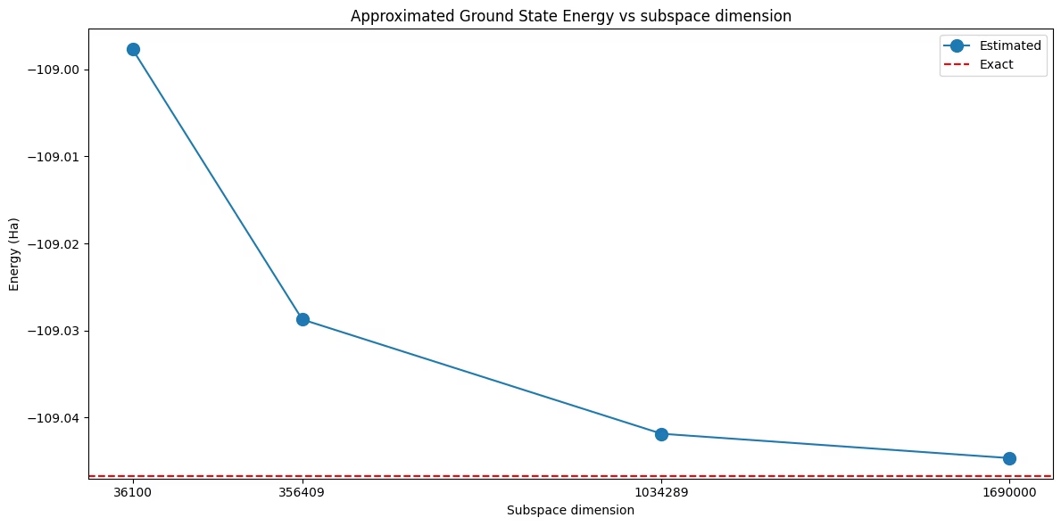
พล็อตนี้แสดงว่าการเพิ่มมิติซับสเปซทำให้ได้ผลลัพธ์ที่แม่นยำขึ้น

import matplotlib.pyplot as plt

# Data for energies plot
x1 = subspace_dimensions
y1 = np.array(energies) + nuclear_repulsion_energy

fig, axs = plt.subplots(1, 1, figsize=(12, 6))

# Plot energies
axs.plot(x1, y1, marker=".", markersize=20, label="Estimated")
axs.set_xticks(x1)
axs.set_xticklabels(x1)
axs.axhline(y=exact_energy, color="red", linestyle="--", label="Exact")
axs.set_title("Approximated Ground State Energy vs subspace dimension")
axs.set_xlabel("Subspace dimension")
axs.set_ylabel("Energy (Ha)")
axs.legend()

plt.tight_layout()
plt.show()

การกำหนดขอบเขตที่ชัดเจนด้วย max_dim

ในการกวาดค่าข้างต้น มิติของซับสเปซถูกควบคุมทางอ้อมเท่านั้น samples_per_batch กำหนดจำนวน bitstring ที่ถูกดึงเข้าแต่ละ batch แต่มิติของซับสเปซที่ได้ขึ้นอยู่กับจำนวนสตริงสปินอัลฟาและสปินเบตาที่ ไม่ซ้ำกัน ที่ bitstring เหล่านั้นมี และพูลของคอนฟิกูเรชันที่ใช้สุ่มย่อยได้จะเพิ่มขึ้นในแต่ละรอบของการกู้คืนคอนฟิกูเรชัน นั่นคือเหตุผลที่มิติซับสเปซบนแกนนอนข้างต้นเป็นตัวเลขที่ไม่สม่ำเสมอซึ่งเราไม่ได้เลือกเอง

อาร์กิวเมนต์ max_dim ของ diagonalize_fermionic_hamiltonian จำกัดมิติโดยตรง มันจำกัดจำนวนสตริง CI ที่เก็บไว้ในแต่ละเซกเตอร์สปิน และเนื่องจากซับสเปซถูกขยายด้วยผลคูณคาร์ทีเซียนของสองเซกเตอร์ มิติของมันจึงเป็นผลคูณของมิติของสองเซกเตอร์:

• max_dim=d จำกัดทั้งสองเซกเตอร์ไว้ที่ d สตริง ดังนั้นมิติซับสเปซจึงมากที่สุด d ** 2

• max_dim=(d_a, d_b) จำกัดเซกเตอร์สปินอัลฟาและสปินเบตาแยกกัน ดังนั้นมิติซับสเปซจึงมากที่สุด d_a * d_b เมื่อ symmetrize_spin=True ขีดจำกัดทั้งสองต้องเท่ากัน

• max_dim=None ซึ่งเป็นค่าเริ่มต้น ไม่กำหนดขีดจำกัด

เมื่อ batch มีสตริงมากกว่าที่ขีดจำกัดอนุญาต สตริงที่สำคัญน้อยที่สุดจะถูกทิ้ง: สตริงที่ส่งผ่าน include_configurations จะถูกเก็บไว้ก่อน ตามด้วยสตริงที่ยกมาจากรอบก่อนหน้า (ดู carryover_threshold) และช่องที่เหลือจะถูกเติมด้วยสตริงที่สุ่มได้เรียงตามความถี่ในการสุ่มจากมากไปน้อย

เนื่องจาก max_dim จำกัดขนาดของการทำ diagonalization ที่ใหญ่ที่สุดที่ตัวแก้ไอเจนสเตตจะถูกขอให้ทำ จึงเป็นวิธีที่สะดวกในการรักษาตัวแก้ให้อยู่ในงบเวลารันและหน่วยความจำ: เลือก samples_per_batch ให้มากเข้าไว้ แล้วให้ max_dim ตัดสินว่าซับสเปซโตได้ใหญ่แค่ไหน

ด้านล่างนี้ เราทำการศึกษาซ้ำ โดยครั้งนี้คงค่า samples_per_batch ไว้และเพิ่ม max_dim

list_max_dim = [100, 200, 400, 800]

# Use a generous number of samples per batch, so that max_dim is what limits
# the dimension of the subspace
samples_per_batch = 600

energies_max_dim = []
subspace_dimensions_max_dim = []

for max_dim in list_max_dim:
    result = diagonalize_fermionic_hamiltonian(
        hcore,
        eri,
        bit_array,
        samples_per_batch=samples_per_batch,
        norb=num_orbitals,
        nelec=(num_elec_a, num_elec_b),
        num_batches=num_batches,
        max_iterations=max_iterations,
        symmetrize_spin=True,
        max_dim=max_dim,
        seed=rng,
    )
    energies_max_dim.append(result.energy)
    subspace_dimensions_max_dim.append(
        int(np.prod(result.sci_state.amplitudes.shape))
    )

print(f"max_dim:            {list_max_dim}")
print(f"subspace dimension: {subspace_dimensions_max_dim}")

max_dim:            [100, 200, 400, 800]
subspace dimension: [10000, 40000, 160000, 640000]

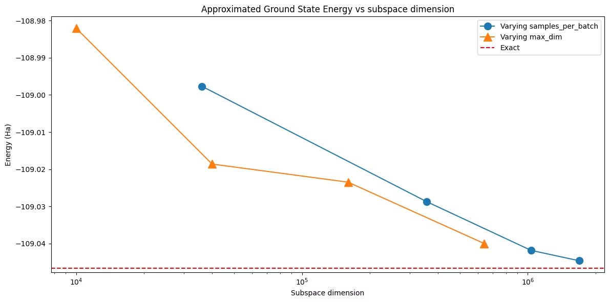
ตอนนี้มิติซับสเปซคือ max_dim ** 2 พอดีในทุกการรัน: มันถูกเลือก ไม่ใช่ถูกค้นพบ การพล็อตการกวาดค่าทั้งสองชุดร่วมกันแสดงว่าความแม่นยำถูกกำหนดโดยมิติซับสเปซเอง ไม่ว่าจะใช้อาร์กิวเมนต์ใดเพื่อไปถึงมิตินั้น อย่างไรก็ตาม เส้นโค้งทั้งสองไม่จำเป็นต้องทับกันพอดี การรันแบบ max_dim สุ่ม 600 bitstring ต่อ batch แล้วเก็บสตริงที่สุ่มได้บ่อยที่สุดไว้ ดังนั้นที่มิติหนึ่ง ๆ มันอาจเก็บชุดคอนฟิกูเรชันที่ดีกว่าการรันที่ไปถึงมิตินั้นด้วยการสุ่ม bitstring น้อยลงตั้งแต่แรก

fig, axs = plt.subplots(1, 1, figsize=(12, 6))

axs.plot(
    subspace_dimensions,
    np.array(energies) + nuclear_repulsion_energy,
    marker=".",
    markersize=20,
    label="Varying samples_per_batch",
)
axs.plot(
    subspace_dimensions_max_dim,
    np.array(energies_max_dim) + nuclear_repulsion_energy,
    marker="^",
    markersize=12,
    label="Varying max_dim",
)
axs.axhline(y=exact_energy, color="red", linestyle="--", label="Exact")
axs.set_xscale("log")
axs.ticklabel_format(axis="y", useOffset=False)
axs.set_title("Approximated Ground State Energy vs subspace dimension")
axs.set_xlabel("Subspace dimension")
axs.set_ylabel("Energy (Ha)")
axs.legend()

plt.tight_layout()
plt.show()