Quantum Variational Circuits และ Quantum Neural Networks

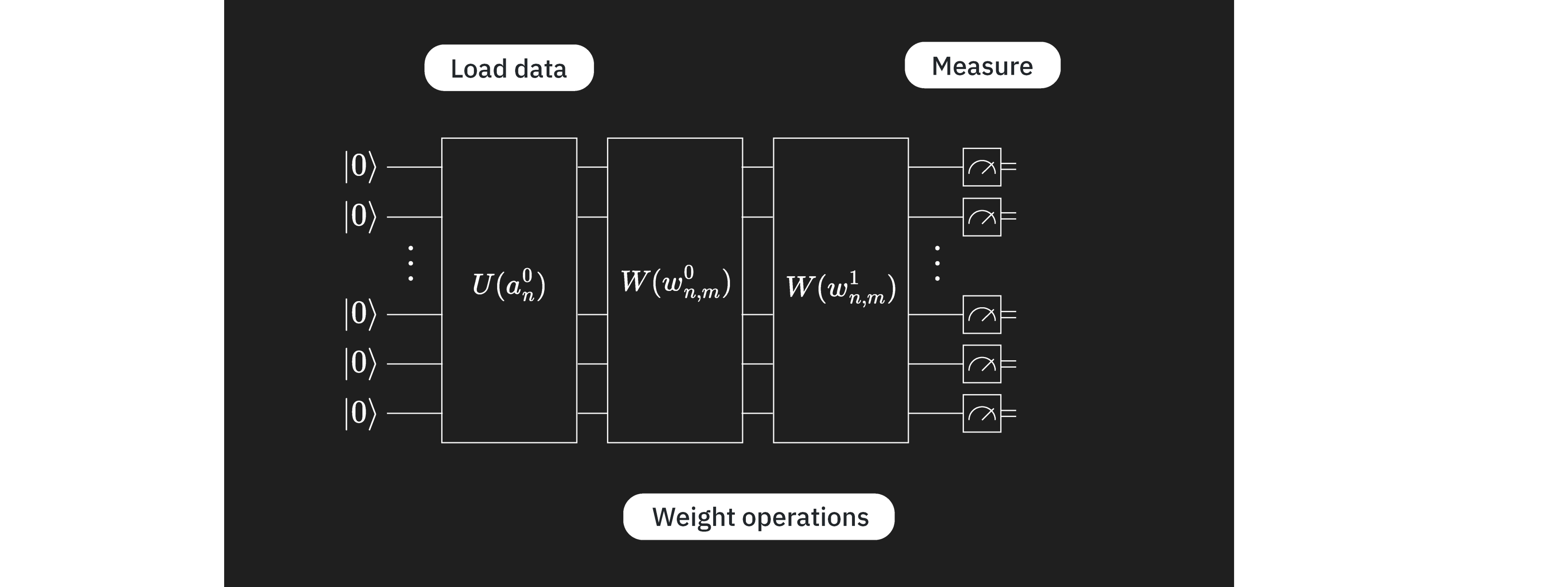
ในบทเรียนนี้ เราจะนำ variational quantum circuits หลายแบบมาใช้กับงานจำแนกประเภทข้อมูล หรือที่เรียกว่า variational quantum classifiers (VQCs) ครั้งหนึ่งเคยเป็นเรื่องปกติที่จะเรียกส่วนหนึ่งของ VQCs ว่า quantum neural networks (QNNs) โดยอ้างอิงถึง neural networks แบบคลาสสิก จริงอยู่ที่มีกรณีที่โครงสร้างที่ยืมมาจาก neural networks แบบคลาสสิก เช่น convolutional layers มีบทบาทสำคัญใน VQCs ในกรณีที่การเปรียบเทียบนั้นแข็งแกร่ง QNNs อาจเป็นคำอธิบายที่มีประโยชน์ แต่ parameterized quantum circuits ไม่จำเป็นต้องทำตามโครงสร้างทั่วไปของ neural network ตัวอย่างเช่น ไม่จำเป็นต้องโหลดข้อมูลทั้งหมดในเลเยอร์แรก (input layer) เราสามารถโหลดข้อมูลบางส่วนในเลเยอร์แรก ใช้ Gate บางอย่าง แล้วโหลดข้อมูลเพิ่มเติม (กระบวนการที่เรียกว่า "reuploading" ข้อมูล) ดังนั้นเราควรคิดว่า QNNs เป็นส่วนหนึ่งของ parameterized quantum circuits และเราไม่ควรถูกจำกัดในการสำรวจ Circuit ควอนตัมที่มีประโยชน์โดยการเปรียบเทียบกับ neural networks แบบคลาสสิก

ชุดข้อมูลที่ใช้ในบทเรียนนี้ประกอบด้วยภาพที่มีแถบแนวนอนและแนวตั้ง และเป้าหมายของเราคือจัดหมวดหมู่ภาพที่ไม่เคยเห็นเข้าหนึ่งในสองหมวดหมู่ตามทิศทางของเส้น เราจะทำสิ่งนี้ด้วย VQC ในขณะที่ดำเนินการ เราจะพูดถึงวิธีที่การคำนวณสามารถปรับปรุงและขยายขนาดได้ ชุดข้อมูลนี้จัดหมวดหมู่ได้ง่ายมากในเชิงคลาสสิก ถูกเลือกเนื่องจากความเรียบง่ายของมัน เพื่อที่เราจะได้โฟกัสที่ส่วนควอนตัมของปัญหา และดูว่าคุณลักษณะของชุดข้อมูลอาจถูกแปลงเป็นส่วนหนึ่งของ Circuit ควอนตัมได้อย่างไร ไม่สมเหตุสมผลที่จะคาดหวังความได้เปรียบเชิงควอนตัมสำหรับกรณีง่ายๆ เช่นนี้ที่อัลกอริทึมแบบคลาสสิกมีประสิทธิภาพสูงมาก

เมื่อจบบทเรียนนี้ คุณควรสามารถ:

โหลดข้อมูลจากภาพเข้าสู่ Circuit ควอนตัม
สร้าง ansatz สำหรับ VQC (หรือ QNN) และปรับให้เหมาะกับปัญหาของคุณ
ฝึก VQC/QNN ของคุณและใช้มันเพื่อทำนายข้อมูลทดสอบได้อย่างแม่นยำ
ขยายปัญหา และรับรู้ขีดจำกัดของคอมพิวเตอร์ควอนตัมปัจจุบัน

การสร้างข้อมูล

เราจะเริ่มต้นด้วยการสร้างข้อมูล ชุดข้อมูลมักไม่ได้ถูกสร้างขึ้นอย่างชัดเจนในฐานะส่วนหนึ่งของ Qiskit patterns framework แต่ประเภทและการเตรียมข้อมูลมีความสำคัญอย่างยิ่งต่อการนำการประมวลผลควอนตัมไปใช้กับ machine learning ได้สำเร็จ โค้ดด้านล่างกำหนดชุดข้อมูลของภาพที่มีขนาด pixel ที่กำหนด แถวหรือคอลัมน์เต็มหนึ่งแถวของภาพจะถูกกำหนดค่า $\pi/2$ และ pixel ที่เหลือจะถูกกำหนดค่าแบบสุ่มในช่วง $(0,\pi/4)$ ค่าแบบสุ่มเหล่านี้คือสัญญาณรบกวนในข้อมูลของเรา ดูโค้ดเพื่อให้แน่ใจว่าคุณเข้าใจวิธีที่ภาพถูกสร้างขึ้น ต่อมาเราจะขยายขนาดภาพ

# Added by doQumentation — required packages for this notebook
!pip install -q matplotlib numpy qiskit qiskit-ibm-runtime scipy scikit-learn

# This code defines the images to be classified:

import numpy as np

# Total number of "pixels"/qubits
size = 8
# One dimension of the image (called vertical, but it doesn't matter). Must be a divisor of `size`
vert_size = 2
# The length of the line to be detected (yellow). Must be less than or equal to the smallest dimension of the image (`<=min(vert_size,size/vert_size)`
line_size = 2

def generate_dataset(num_images):
    images = []
    labels = []
    hor_array = np.zeros((size - (line_size - 1) * vert_size, size))
    ver_array = np.zeros((round(size / vert_size) * (vert_size - line_size + 1), size))

    j = 0
    for i in range(0, size - 1):
        if i % (size / vert_size) <= (size / vert_size) - line_size:
            for p in range(0, line_size):
                hor_array[j][i + p] = np.pi / 2
            j += 1

    # Make two adjacent entries pi/2, then move down to the next row. Careful to avoid the "pixels" at size/vert_size - linesize, because we want to fold this list into a grid.

    j = 0
    for i in range(0, round(size / vert_size) * (vert_size - line_size + 1)):
        for p in range(0, line_size):
            ver_array[j][i + p * round(size / vert_size)] = np.pi / 2
        j += 1

    # Make entries pi/2, spaced by the length/rows, so that when folded, the entries appear on top of each other.

    for n in range(num_images):
        rng = np.random.randint(0, 2)
        if rng == 0:
            labels.append(-1)
            random_image = np.random.randint(0, len(hor_array))
            images.append(np.array(hor_array[random_image]))

        elif rng == 1:
            labels.append(1)
            random_image = np.random.randint(0, len(ver_array))
            images.append(np.array(ver_array[random_image]))
            # Randomly select 0 or 1 for a horizontal or vertical array, assign the corresponding label.

        # Create noise
        for i in range(size):
            if images[-1][i] == 0:
                images[-1][i] = np.random.rand() * np.pi / 4
    return images, labels

hor_size = round(size / vert_size)

โปรดทราบว่าโค้ดข้างต้นยังสร้าง label ที่บ่งบอกว่าภาพมีเส้นแนวตั้ง (+1) หรือแนวนอน (-1) ตอนนี้เราจะใช้ sklearn แบ่งชุดข้อมูล 100 ภาพออกเป็นชุดฝึกและชุดทดสอบ (พร้อม label ที่สอดคล้องกัน) ที่นี่เราใช้ $70%$ ของชุดข้อมูลสำหรับการฝึก โดยเก็บ $30%$ ที่เหลือไว้สำหรับการทดสอบ

from sklearn.model_selection import train_test_split

np.random.seed(42)
images, labels = generate_dataset(200)

train_images, test_images, train_labels, test_labels = train_test_split(
    images, labels, test_size=0.3, random_state=246
)

มาพล็อตองค์ประกอบบางส่วนของชุดข้อมูลเพื่อดูว่าเส้นเหล่านี้มีลักษณะอย่างไร:

import matplotlib.pyplot as plt

# Make subplot titles so we can identify categories
titles = []
for i in range(8):
    title = "category: " + str(train_labels[i])
    titles.append(title)

# Generate a figure with nested images using subplots.
fig, ax = plt.subplots(4, 2, figsize=(10, 6), subplot_kw={"xticks": [], "yticks": []})

for i in range(8):
    ax[i // 2, i % 2].imshow(
        train_images[i].reshape(vert_size, hor_size),
        aspect="equal",
    )
    ax[i // 2, i % 2].set_title(titles[i])
plt.subplots_adjust(wspace=0.1, hspace=0.3)

Output of the previous code cell

ภาพแต่ละภาพยังคู่กับ label ใน train_labels อยู่ในรูปแบบลิสต์ธรรมดา:

print(train_labels[:8])

[1, 1, 1, 1, -1, 1, 1, 1]

Variational quantum classifier: ความพยายามแรก

Qiskit patterns ขั้นตอนที่ 1: แมปปัญหาเป็น Circuit ควอนตัม

เป้าหมายคือการหาฟังก์ชัน $f$ ที่มีพารามิเตอร์ $\theta$ ซึ่งแมปเวกเตอร์ข้อมูล/ภาพ $\vec{x}$ ไปยังหมวดหมู่ที่ถูกต้อง: $f_\theta(\vec{x}) \rightarrow \pm1$ สิ่งนี้จะทำด้วย VQC ที่มีเลเยอร์น้อย ซึ่งสามารถระบุได้จากวัตถุประสงค์ที่แตกต่างกัน:

f_\theta(\vec{x}) = \langle 0|U^{\dagger}(\vec{x})W^\dagger(\theta)OW(\theta)U(\vec{x})|0\rangle

ที่นี่ $U(\vec{x})$ คือ Circuit การเข้ารหัส ซึ่งมีตัวเลือกมากมายดังที่เห็นในบทเรียนก่อนหน้า $W(\theta)$ คือบล็อก Circuit แบบ variational หรือ trainable และ $\theta$ คือชุดพารามิเตอร์ที่จะฝึก พารามิเตอร์เหล่านั้นจะถูกปรับแปรโดย optimizer แบบคลาสสิกเพื่อหาชุดพารามิเตอร์ที่ให้การจำแนกประเภทภาพที่ดีที่สุดโดย Circuit ควอนตัม variational circuit นี้บางครั้งเรียกว่า "ansatz" สุดท้าย $O$ คือ observable บางอย่างที่จะประมาณโดยใช้ primitive Estimator ไม่มีข้อจำกัดที่บังคับให้เลเยอร์ต้องมาในลำดับนี้ หรือแม้แต่ต้องแยกออกจากกันโดยสมบูรณ์ เราสามารถมีเลเยอร์ variational และ/หรือ encoding หลายชั้นในลำดับใดก็ได้ที่มีแรงจูงใจทางเทคนิค

เราเริ่มต้นด้วยการเลือกแผนที่ฟีเจอร์เพื่อเข้ารหัสข้อมูลของเรา เราจะใช้ z_feature_map เนื่องจากช่วยให้ความลึกของ Circuit ต่ำเมื่อเทียบกับการแมปฟีเจอร์อื่นๆ

from qiskit.circuit.library import z_feature_map

# One qubit per data feature
num_qubits = len(train_images[0])

# Data encoding
# Note that qiskit orders parameters alphabetically. We assign the parameter prefix "a" to ensure our data encoding goes to the first part of the circuit, the feature mapping.
feature_map = z_feature_map(num_qubits, parameter_prefix="a")

ตอนนี้เราต้องตัดสินใจเกี่ยวกับ ansatz ที่จะฝึก มีการพิจารณาหลายอย่างในการเลือก ansatz คำอธิบายที่สมบูรณ์เกินขอบเขตของบทนำนี้ ที่นี่เราเพียงชี้ให้เห็นหมวดหมู่การพิจารณาบางอย่าง

ฮาร์ดแวร์: คอมพิวเตอร์ควอนตัมสมัยใหม่ทั้งหมดเสี่ยงต่อข้อผิดพลาดและสัญญาณรบกวนมากกว่าคู่แบบคลาสสิก การใช้ ansatz ที่ลึกเกินไป (โดยเฉพาะในความลึก two-qubit transpiled) จะไม่ให้ผลลัพธ์ที่ดี ปัญหาที่เกี่ยวข้องคือคอมพิวเตอร์ควอนตัมมี qubit layout บางอย่าง หมายความว่า Qubit ทางกายภาพบางตัวอยู่ติดกันบนคอมพิวเตอร์ควอนตัม และบางตัวอาจอยู่ห่างกันมาก การพัวพัน Qubit ที่อยู่ติดกันไม่เพิ่มความลึกมากนัก แต่การพัวพัน Qubit ที่อยู่ห่างกันมากอาจเพิ่มความลึกได้อย่างมาก เนื่องจากเราต้องใส่ swap gates เพื่อย้ายข้อมูลไปยัง Qubit ที่อยู่ติดกันเพื่อให้สามารถพัวพันได้
ปัญหา: เมื่อใดก็ตามที่คุณมีข้อมูลบางอย่างเกี่ยวกับปัญหาที่สามารถชี้แนะ ansatz ของคุณ ให้ใช้มัน ตัวอย่างเช่น ข้อมูลในบทเรียนนี้ประกอบด้วยภาพของเส้นแนวนอนและแนวตั้ง เราสามารถพิจารณาว่าความสัมพันธ์ระหว่างสีที่อยู่ติดกัน/ค่าที่ระบุภาพของเส้นแนวนอนหรือแนวตั้งคืออะไร คุณสมบัติใดของ ansatz จะสอดคล้องกับความสัมพันธ์นี้ระหว่าง pixel ที่อยู่ติดกัน? เราจะกลับมาที่ประเด็นนี้ในเชิงเทคนิคมากขึ้นในภายหลังในบทเรียนนี้ แต่ตอนนี้ขอแค่บอกว่าการรวม entanglement และ CNOT gates ระหว่าง Qubit ที่สอดคล้องกับ pixel ที่อยู่ติดกันดูเหมือนเป็นความคิดที่ดี ในภาพรวม พิจารณาว่าปัญหานั้นแก้ได้ดีที่สุดด้วย Circuit ควอนตัมจริงๆ หรือไม่ หรือมีอัลกอริทึมแบบคลาสสิกที่สามารถทำงานได้ดีพอๆ กัน
จำนวนพารามิเตอร์: Gate ควอนตัมที่มีพารามิเตอร์อิสระแต่ละตัวใน Circuit จะเพิ่มพื้นที่ที่ต้องปรับให้เหมาะสมแบบคลาสสิก ซึ่งส่งผลให้การ converge ช้าลง แต่เมื่อปัญหาขยายขนาดขึ้น เราอาจพบ barren plateaus คำนี้หมายถึงปรากฏการณ์ที่ภูมิทัศน์การปรับของอัลกอริทึมควอนตัม variational กลายเป็นแบน flat และไม่มีลักษณะเด่นแบบ exponential เมื่อขนาดปัญหาเพิ่มขึ้น ส่งผลให้ gradient หายไป ทำให้ยากต่อการฝึกอัลกอริทึมได้อย่างมีประสิทธิภาพ[1] Barren plateaus เกี่ยวข้องกับอัลกอริทึมควอนตัม variational อย่าง VQCs/QNNs ควรทราบว่าจำนวนพารามิเตอร์ที่เพิ่มขึ้นไม่ใช่การพิจารณาเดียวในการหลีกเลี่ยง barren plateaus การพิจารณาอื่นๆ ได้แก่ cost functions แบบ global และการกำหนดค่าพารามิเตอร์เริ่มต้นแบบสุ่ม

ในบทเรียนนี้ เราจะเห็นตัวอย่างง่ายๆ ของการปฏิบัติที่ดีในการสร้าง ansatz มาลองใช้ ansatz ด้านล่างก่อน เราจะกลับมาแก้ไขในภายหลัง

# Import the necessary packages
from qiskit import QuantumCircuit
from qiskit.circuit import ParameterVector

# Initialize the circuit using the same number of qubits as the image has pixels
qnn_circuit = QuantumCircuit(size)

# We choose to have two variational parameters for each qubit.
params = ParameterVector("θ", length=2 * size)

# A first variational layer:
for i in range(size):
    qnn_circuit.ry(params[i], i)

# Here is a list of qubit pairs between which we want CNOT gates. The choice of these is not yet obvious.
qnn_cnot_list = [[0, 1], [1, 2], [2, 3]]

for i in range(len(qnn_cnot_list)):
    qnn_circuit.cx(qnn_cnot_list[i][0], qnn_cnot_list[i][1])

# The second variational layer:
for i in range(size):
    qnn_circuit.rx(params[size + i], i)

# Check the circuit depth, and the two-qubit gate depth
print(qnn_circuit.decompose().depth())
print(
    f"2+ qubit depth: {qnn_circuit.decompose().depth(lambda instr: len(instr.qubits) > 1)}"
)

# Draw the circuit
qnn_circuit.draw("mpl")

5
2+ qubit depth: 3

┌──────────┐             ┌──────────┐
q_0: ┤ Ry(θ[0]) ├──────■──────┤ Rx(θ[8]) ├─────────────────────────
     ├──────────┤    ┌─┴─┐    └──────────┘┌──────────┐
q_1: ┤ Ry(θ[1]) ├────┤ X ├─────────■──────┤ Rx(θ[9]) ├─────────────
     ├──────────┤    └───┘       ┌─┴─┐    └──────────┘┌───────────┐
q_2: ┤ Ry(θ[2]) ├────────────────┤ X ├─────────■──────┤ Rx(θ[10]) ├
     ├──────────┤                └───┘       ┌─┴─┐    ├───────────┤
q_3: ┤ Ry(θ[3]) ├────────────────────────────┤ X ├────┤ Rx(θ[11]) ├
     ├──────────┤┌───────────┐               └───┘    └───────────┘
q_4: ┤ Ry(θ[4]) ├┤ Rx(θ[12]) ├─────────────────────────────────────
     ├──────────┤├───────────┤
q_5: ┤ Ry(θ[5]) ├┤ Rx(θ[13]) ├─────────────────────────────────────
     ├──────────┤├───────────┤
q_6: ┤ Ry(θ[6]) ├┤ Rx(θ[14]) ├─────────────────────────────────────
     ├──────────┤├───────────┤
q_7: ┤ Ry(θ[7]) ├┤ Rx(θ[15]) ├─────────────────────────────────────
     └──────────┘└───────────┘

เมื่อเตรียม Circuit การเข้ารหัสข้อมูลและ variational circuit แล้ว เราสามารถรวมกันเพื่อสร้าง ansatz เต็มรูปแบบ ในกรณีนี้ องค์ประกอบของ Circuit ควอนตัมของเราค่อนข้างคล้ายกับเลเยอร์ใน neural networks โดย $U(\vec{x})$ คล้ายกับเลเยอร์ที่โหลดค่าอินพุตจากภาพมากที่สุด และ $W(\theta)$ คล้ายกับเลเยอร์ของ "weights" แบบตัวแปร เนื่องจากการเปรียบเทียบนี้ใช้ได้ในกรณีนี้ เราจึงนำ "qnn" มาใช้ในบางชื่อตัวแปร แต่การเปรียบเทียบนี้ไม่ควรจำกัดการสำรวจ VQCs ของคุณ

# QNN ansatz
ansatz = qnn_circuit

# Combine the feature map with the ansatz
full_circuit = QuantumCircuit(num_qubits)
full_circuit.compose(feature_map, range(num_qubits), inplace=True)
full_circuit.compose(ansatz, range(num_qubits), inplace=True)

# Display the circuit
full_circuit.decompose().draw("mpl", style="clifford", fold=-1)

Output of the previous code cell

ตอนนี้เราต้องกำหนด observable เพื่อใช้ใน cost function เราจะได้ค่าความคาดหวังสำหรับ observable นี้โดยใช้ Estimator ถ้าเราเลือก ansatz ที่ดีและมีแรงจูงใจจากปัญหา แต่ละ Qubit จะมีข้อมูลที่เกี่ยวข้องกับการจำแนกประเภท เราสามารถเพิ่มเลเยอร์เพื่อรวมข้อมูลไปยัง Qubit จำนวนน้อยลง (เรียกว่า convolutional layer) เพื่อให้การวัดจำเป็นเฉพาะบน Qubit ส่วนหนึ่งของ Circuit เท่านั้น (เช่นใน convolutional neural networks) หรือเราสามารถวัดคุณสมบัติบางอย่างจากแต่ละ Qubit ที่นี่เราเลือกแบบหลัง ดังนั้นเราจึงรวม operator Z สำหรับแต่ละ Qubit ไม่มีอะไรพิเศษเกี่ยวกับการเลือก $Z$ แต่มีเหตุผลที่ดี:

นี่เป็นงานจำแนกประเภทไบนารี และการวัด $Z$ สามารถให้ผลลัพธ์สองแบบที่เป็นไปได้
eigenvalues ของ $Z$ ( $\pm 1$ ) ถูกแยกออกจากกันอย่างสมเหตุสมผล และส่งผลให้ผลลัพธ์ Estimator อยู่ในช่วง [-1, +1] โดยที่ 0 สามารถใช้เป็นค่าตัดได้ง่ายๆ
วัดในฐาน Pauli Z ได้ตรงๆ โดยไม่ต้องเพิ่ม Gate overhead

ดังนั้น Z จึงเป็นตัวเลือกที่เป็นธรรมชาติมาก

from qiskit.quantum_info import SparsePauliOp

observable = SparsePauliOp.from_list([("Z" * (num_qubits), 1)])

เรามี Circuit ควอนตัมและ observable ที่ต้องการประมาณแล้ว ตอนนี้เราต้องการสิ่งต่างๆ เพื่อรันและปรับ Circuit นี้ ขั้นแรก เราต้องการฟังก์ชันเพื่อรัน forward pass โปรดทราบว่าฟังก์ชันด้านล่างรับ input_params และ weight_params แยกกัน อย่างแรกคือชุดพารามิเตอร์คงที่ที่อธิบายข้อมูลในภาพ และอย่างหลังคือชุดพารามิเตอร์ตัวแปรที่ต้องปรับให้เหมาะสม

from qiskit.primitives import BaseEstimatorV2
from qiskit.quantum_info.operators.base_operator import BaseOperator

def forward(
    circuit: QuantumCircuit,
    input_params: np.ndarray,
    weight_params: np.ndarray,
    estimator: BaseEstimatorV2,
    observable: BaseOperator,
) -> np.ndarray:
    """
    Forward pass of the neural network.

    Args:
        circuit: circuit consisting of data loader gates and the neural network ansatz.
        input_params: data encoding parameters.
        weight_params: neural network ansatz parameters.
        estimator: EstimatorV2 primitive.
        observable: a single observable to compute the expectation over.

    Returns:
        expectation_values: an array (for one observable) or a matrix (for a sequence of observables) of expectation values.
        Rows correspond to observables and columns to data samples.
    """
    num_samples = input_params.shape[0]
    weights = np.broadcast_to(weight_params, (num_samples, len(weight_params)))
    params = np.concatenate((input_params, weights), axis=1)
    pub = (circuit, observable, params)
    job = estimator.run([pub])
    result = job.result()[0]
    expectation_values = result.data.evs

    return expectation_values

Loss function

ต่อมาเราต้องการ loss function เพื่อคำนวณความแตกต่างระหว่างค่าที่ทำนายและค่าที่คำนวณได้ของ label ฟังก์ชันจะรับ label ที่ทำนายโดยอัลกอริทึมและ label ที่ถูกต้อง แล้วคืนค่าความแตกต่างกำลังสองเฉลี่ย มี loss function หลายแบบ ที่นี่ MSE เป็นตัวอย่างที่เราเลือก

def mse_loss(predict: np.ndarray, target: np.ndarray) -> np.ndarray:
    """
    Mean squared error (MSE).

    prediction: predictions from the forward pass of neural network.
    target: true labels.

    output: MSE loss.
    """
    if len(predict.shape) <= 1:
        return ((predict - target) ** 2).mean()
    else:
        raise AssertionError("input should be 1d-array")

มากำหนด loss function ที่แตกต่างกันเล็กน้อยซึ่งเป็นฟังก์ชันของพารามิเตอร์ตัวแปร (weights) เพื่อใช้โดย optimizer แบบคลาสสิก ฟังก์ชันนี้รับเฉพาะพารามิเตอร์ ansatz เป็นอินพุต ตัวแปรอื่นๆ สำหรับ forward pass และ loss ถูกตั้งเป็นพารามิเตอร์ global optimizer จะฝึกโมเดลโดยสุ่มตัวอย่าง weights ที่แตกต่างกันและพยายามลดเอาต์พุตของ cost/loss function

def mse_loss_weights(weight_params: np.ndarray) -> np.ndarray:
    """
    Cost function for the optimizer to update the ansatz parameters.

    weight_params: ansatz parameters to be updated by the optimizer.

    output: MSE loss.
    """
    predictions = forward(
        circuit=circuit,
        input_params=input_params,
        weight_params=weight_params,
        estimator=estimator,
        observable=observable,
    )

    cost = mse_loss(predict=predictions, target=target)
    objective_func_vals.append(cost)

    global iter
    if iter % 50 == 0:
        print(f"Iter: {iter}, loss: {cost}")
    iter += 1

    return cost

ข้างต้นเราอ้างถึงการใช้ optimizer แบบคลาสสิก เมื่อเราค้นหา weights เพื่อลด cost function เราจะใช้ optimizer COBYLA:

from scipy.optimize import minimize

เราจะตั้งค่าตัวแปร global เริ่มต้นสำหรับ cost function

# Globals
circuit = full_circuit
observables = observable
# input_params = train_images_batch
# target = train_labels_batch
objective_func_vals = []
iter = 0

Qiskit Patterns ขั้นตอนที่ 2: ปรับปัญหาให้เหมาะสมสำหรับการประมวลผลควอนตัม

เราเริ่มต้นด้วยการเลือก Backend สำหรับการประมวลผล ในกรณีนี้ เราจะใช้ Backend ที่ว่างที่สุด

from qiskit_ibm_runtime import QiskitRuntimeService

service = QiskitRuntimeService()
backend = service.least_busy(operational=True, simulator=False)
print(backend.name)

ibm_brisbane

ที่นี่เราปรับ Circuit สำหรับการรันบน Backend จริงโดยระบุ optimization_level และเพิ่ม dynamical decoupling โค้ดด้านล่างสร้าง pass manager โดยใช้ preset pass managers จาก qiskit.transpiler

from qiskit.circuit.library import XGate
from qiskit.transpiler import PassManager
from qiskit.transpiler.passes import (
    ALAPScheduleAnalysis,
    ConstrainedReschedule,
    PadDynamicalDecoupling,
)
from qiskit.transpiler.preset_passmanagers import generate_preset_pass_manager

target = backend.target

pm = generate_preset_pass_manager(target=target, optimization_level=3)
pm.scheduling = PassManager(
    [
        ALAPScheduleAnalysis(target=target),
        ConstrainedReschedule(
            acquire_alignment=target.acquire_alignment,
            pulse_alignment=target.pulse_alignment,
            target=target,
        ),
        PadDynamicalDecoupling(
            target=target,
            dd_sequence=[XGate(), XGate()],
            pulse_alignment=target.pulse_alignment,
        ),
    ]
)

ตอนนี้เราใช้ pass manager บน Circuit การเปลี่ยนแปลง layout ที่เกิดขึ้นต้องนำไปใช้กับ observable ด้วย สำหรับ Circuit ขนาดใหญ่มาก heuristics ที่ใช้ในการปรับ Circuit อาจไม่ให้ Circuit ที่ดีที่สุดและตื้นที่สุดเสมอไป ในกรณีเหล่านั้น การรัน pass managers หลายครั้งและใช้ Circuit ที่ดีที่สุดเป็นเรื่องสมเหตุสมผล เราจะเห็นสิ่งนี้ในภายหลังเมื่อเราขยายการคำนวณ

circuit_ibm = pm.run(full_circuit)
observable_ibm = observable.apply_layout(circuit_ibm.layout)

Qiskit Patterns ขั้นตอนที่ 3: ประมวลผลโดยใช้ Qiskit Primitives

วนซ้ำชุดข้อมูลเป็น batch และ epoch

ก่อนอื่นเราจะนำอัลกอริทึมทั้งหมดมาใช้โดยใช้ซิมูเลเตอร์เพื่อ debug เบื้องต้นและประมาณค่าข้อผิดพลาด ตอนนี้เราสามารถผ่านชุดข้อมูลทั้งหมดเป็น batch ในจำนวน epoch ที่ต้องการเพื่อฝึก quantum neural network

from qiskit.primitives import StatevectorEstimator as Estimator

batch_size = 140
num_epochs = 1
num_samples = len(train_images)

# Globals
circuit = full_circuit
estimator = Estimator()  # simulator for debugging
observables = observable
objective_func_vals = []
iter = 0

# Random initial weights for the ansatz
np.random.seed(42)
weight_params = np.random.rand(len(ansatz.parameters)) * 2 * np.pi

for epoch in range(num_epochs):
    for i in range((num_samples - 1) // batch_size + 1):
        print(f"Epoch: {epoch}, batch: {i}")
        start_i = i * batch_size
        end_i = start_i + batch_size
        train_images_batch = np.array(train_images[start_i:end_i])
        train_labels_batch = np.array(train_labels[start_i:end_i])
        input_params = train_images_batch
        target = train_labels_batch
        iter = 0
        res = minimize(
            mse_loss_weights, weight_params, method="COBYLA", options={"maxiter": 100}
        )
        weight_params = res["x"]

Epoch: 0, batch: 0
Iter: 0, loss: 1.0002309063537163
Iter: 50, loss: 0.9434121445008878

Qiskit Patterns ขั้นตอนที่ 4: ประมวลผลหลังการวัด คืนผลลัพธ์ในรูปแบบคลาสสิก

การทดสอบและความแม่นยำ

ตอนนี้เราตีความผลลัพธ์จากการฝึก เราทดสอบความแม่นยำการฝึกบนชุดข้อมูลการฝึกก่อน

import copy
from sklearn.metrics import accuracy_score
from qiskit.primitives import StatevectorEstimator as Estimator  # simulator
# from qiskit_ibm_runtime import EstimatorV2 as Estimator  # real quantum computer

estimator = Estimator()
# estimator = Estimator(backend=backend)

pred_train = forward(circuit, np.array(train_images), res["x"], estimator, observable)
# pred_train = forward(circuit_ibm, np.array(train_images), res['x'], estimator, observable_ibm)

print(pred_train)

pred_train_labels = copy.deepcopy(pred_train)
pred_train_labels[pred_train_labels >= 0] = 1
pred_train_labels[pred_train_labels < 0] = -1
print(pred_train_labels)
print(train_labels)

accuracy = accuracy_score(train_labels, pred_train_labels)
print(f"Train accuracy: {accuracy * 100}%")

[-2.27688499e-02 -1.46227204e-02 -1.73927452e-02  9.93331786e-02
 -4.85553548e-01  1.43558565e-01  8.34567054e-02 -1.40133992e-02
  1.52169596e-01 -1.95082515e-01  8.24373578e-03 -9.90696638e-02
 -3.54268344e-02 -4.77017954e-01  1.38713848e-02 -2.99706215e-01
 -5.78378029e-02  3.25528779e-02 -4.11354239e-02 -1.06483708e-01
  1.53095800e-01  2.90110884e-02  1.25745450e-02  6.46323079e-02
 -1.53538943e-01 -1.57694952e-02 -1.67800067e-02 -1.99820822e-01
  1.70360075e-01  7.86148038e-03 -2.33373818e-02  6.64233020e-02
 -1.14895445e-01 -1.11296215e-01  1.15120303e-01 -2.94096140e-01
 -1.00531392e-03 -1.69209726e-01 -1.26120885e-01  3.26298176e-02
 -1.33517383e-02 -5.86983444e-02 -4.32341361e-01 -4.36509551e-01
 -4.17940102e-02  1.76935235e-03  8.14479984e-03  1.86985655e-01
 -2.75525019e-01 -1.63229907e-03 -1.08571055e-01 -7.37452387e-04
 -6.44440657e-02  6.72812834e-04  2.16785530e-03  1.41381850e-01
 -9.82570410e-02  4.35973325e-01 -7.62261965e-02 -1.86193980e-01
 -1.56971183e-02 -4.02757541e-01 -1.53869367e-01  2.29262129e-02
 -7.02788246e-03  3.65719683e-02  4.68232163e-01  2.36434668e-02
 -2.59520939e-02  3.70550137e-01 -1.19630110e-01 -5.79555318e-02
  2.09554455e-01  5.04689780e-02  7.39494314e-02 -1.77647326e-02
 -1.45407207e-01 -9.54908878e-02  7.56029640e-02 -2.74049696e-02
  3.34885873e-01  1.58546171e-03  1.09339091e-01 -8.84693274e-02
 -2.36450457e-02  1.41892239e-01 -2.34453218e-01 -7.50717757e-02
 -1.13281310e-01 -1.66649414e-01 -3.17224197e-01 -6.38220597e-02
  3.28916563e-02  3.04739203e-02  2.67720196e-02 -1.16485785e-01
 -3.08115732e-02 -2.95372010e-02 -7.54669023e-02  6.20013872e-02
 -3.85258710e-01 -1.16456443e-01 -7.38548075e-02 -3.20558243e-02
 -4.22284741e-02  1.01285659e-01 -1.76949246e-01 -2.02767491e-01
 -1.12407344e-01 -3.81408267e-02 -4.33345231e-01 -9.24507501e-02
 -4.21765393e-02 -6.06533771e-02 -2.22257783e-01 -1.17312535e-01
 -6.74132262e-02 -2.76206274e-01 -9.13971800e-02 -2.27653991e-01
  1.66358563e-01  2.17230774e-04  5.76426304e-02 -2.82079169e-02
 -1.15482051e-01 -3.46716009e-01 -3.21448755e-01 -5.20041405e-02
 -2.16833625e-01 -1.06154654e-02 -7.74854811e-02 -3.28257935e-01
 -7.83242410e-02  1.65547682e-01 -2.55294862e-01 -8.89085025e-02
  4.47581491e-01  1.92351832e-02  2.74083885e-02 -3.61304571e-01]
[-1. -1. -1.  1. -1.  1.  1. -1.  1. -1.  1. -1. -1. -1.  1. -1. -1.  1.
 -1. -1.  1.  1.  1.  1. -1. -1. -1. -1.  1.  1. -1.  1. -1. -1.  1. -1.
 -1. -1. -1.  1. -1. -1. -1. -1. -1.  1.  1.  1. -1. -1. -1. -1. -1.  1.
  1.  1. -1.  1. -1. -1. -1. -1. -1.  1. -1.  1.  1.  1. -1.  1. -1. -1.
  1.  1.  1. -1. -1. -1.  1. -1.  1.  1.  1. -1. -1.  1. -1. -1. -1. -1.
 -1. -1.  1.  1.  1. -1. -1. -1. -1.  1. -1. -1. -1. -1. -1.  1. -1. -1.
 -1. -1. -1. -1. -1. -1. -1. -1. -1. -1. -1. -1.  1.  1.  1. -1. -1. -1.
 -1. -1. -1. -1. -1. -1. -1.  1. -1. -1.  1.  1.  1. -1.]
[1, 1, 1, 1, -1, 1, 1, 1, -1, 1, 1, 1, -1, -1, -1, -1, -1, -1, -1, -1, 1, -1, 1, 1, -1, 1, 1, 1, 1, -1, 1, 1, -1, 1, 1, -1, 1, 1, -1, -1, -1, 1, -1, -1, 1, -1, 1, 1, -1, 1, -1, 1, 1, -1, 1, 1, 1, 1, -1, -1, -1, -1, 1, -1, 1, 1, 1, -1, -1, 1, 1, -1, 1, 1, -1, -1, 1, -1, 1, 1, 1, 1, 1, -1, -1, 1, -1, -1, -1, -1, -1, 1, 1, -1, -1, 1, -1, -1, 1, 1, -1, 1, -1, 1, 1, 1, 1, 1, -1, -1, -1, 1, -1, -1, -1, 1, -1, -1, 1, -1, 1, -1, 1, 1, -1, -1, -1, 1, 1, 1, -1, -1, -1, 1, -1, 1, 1, -1, -1, -1]
Train accuracy: 60.0%

ความแม่นยำในการฝึกอยู่ที่เพียง $60%$ ซึ่งไม่ดีอย่างแน่นอน ยากที่จะจินตนาการว่าประสิทธิภาพของโมเดลบนชุดทดสอบจะดีกว่า มาตรวจสอบดู

pred_test = forward(circuit, np.array(test_images), res["x"], estimator, observable)
# pred_test = forward(circuit_ibm, np.array(test_images), res['x'], estimator, observable_ibm)

print(pred_test)

pred_test_labels = copy.deepcopy(pred_test)
pred_test_labels[pred_test_labels >= 0] = 1
pred_test_labels[pred_test_labels < 0] = -1
print(pred_test_labels)
print(test_labels)

accuracy = accuracy_score(test_labels, pred_test_labels)
print(f"Test accuracy: {accuracy * 100}%")

[-2.77978120e-01 -2.62194862e-01  4.59636095e-02 -8.09344165e-02
 -2.97362966e-01  9.22947242e-02  2.06693174e-01  3.31629460e-02
  1.10971762e-03 -2.14602152e-01 -1.62671993e-01 -6.07179155e-04
 -1.59948633e-01 -8.55722523e-02 -1.13057027e-01 -3.00187433e-01
 -2.92832827e-01  7.38580629e-02 -6.03706270e-02 -8.57643552e-02
 -1.52402062e-02 -3.57505447e-01 -3.54890597e-02  1.36534749e-01
 -1.54688180e-01 -2.93714726e-01  1.89548513e-02 -6.15715564e-02
  1.11042670e-01 -2.22861100e-02 -3.84230105e-02  1.67351034e-01
 -8.38766333e-02  2.56348613e-01 -1.10653111e-01 -1.18989476e-01
 -6.75723266e-05 -6.88580547e-02  1.02431393e-02 -2.42125353e-01
 -1.09142367e-01 -1.22540757e-01 -1.63735850e-01  3.93334838e-01
  2.36705685e-01 -2.34259814e-02 -3.91877756e-02 -1.95106746e-01
  1.86707523e-01  4.74775215e-02 -4.24907432e-02 -2.06453265e-01
  4.09184710e-02 -3.54762080e-02 -9.47513112e-02  2.97270112e-01
 -2.99708696e-02  9.93941064e-03 -1.26760302e-01 -1.36183355e-01]
[-1. -1.  1. -1. -1.  1.  1.  1.  1. -1. -1. -1. -1. -1. -1. -1. -1.  1.
 -1. -1. -1. -1. -1.  1. -1. -1.  1. -1.  1. -1. -1.  1. -1.  1. -1. -1.
 -1. -1.  1. -1. -1. -1. -1.  1.  1. -1. -1. -1.  1.  1. -1. -1.  1. -1.
 -1.  1. -1.  1. -1. -1.]
[-1, -1, 1, 1, -1, -1, 1, -1, 1, -1, 1, 1, 1, 1, -1, 1, -1, 1, 1, 1, 1, -1, -1, 1, 1, -1, 1, 1, 1, -1, 1, -1, -1, 1, 1, 1, -1, 1, 1, -1, -1, -1, 1, 1, 1, -1, 1, 1, 1, 1, -1, -1, 1, 1, 1, 1, 1, 1, -1, -1]
Test accuracy: 60.0%

โมเดลไม่ได้จำแนกข้อมูลเหล่านี้ได้ดี เราควรถามว่าทำไม และโดยเฉพาะ เราควรตรวจสอบ:

เราหยุดการฝึกเร็วเกินไปหรือไม่? ต้องการขั้นตอนการปรับให้เหมาะสมมากขึ้นหรือเปล่า?
เราสร้าง ansatz ที่ไม่ดีหรือไม่? ซึ่งอาจหมายถึงหลายอย่าง เมื่อเราทำงานบนคอมพิวเตอร์ควอนตัมจริง ความลึกของ Circuit จะเป็นการพิจารณาหลัก จำนวนพารามิเตอร์ก็อาจมีความสำคัญเช่นกัน รวมถึงการพัวพันระหว่าง Qubit
รวมสองข้อข้างต้น เราสร้าง ansatz ที่มีพารามิเตอร์มากเกินไปจนไม่สามารถฝึกได้หรือไม่?

เราสามารถเริ่มต้นด้วยการตรวจสอบ convergence ในการปรับให้เหมาะสม:

obj_func_vals_first = objective_func_vals
# import matplotlib.pyplot as plt

plt.figure(figsize=(12, 6))
plt.plot(obj_func_vals_first, label="first ansatz")
plt.xlabel("iteration")
plt.ylabel("loss")
plt.legend()
plt.show()

Output of the previous code cell

เราอาจลองขยายขั้นตอนการปรับให้เหมาะสมเพื่อให้แน่ใจว่า optimizer ไม่ได้ติดค้างอยู่ใน local minimum ในพื้นที่พารามิเตอร์ แต่ดูเหมือนค่อนข้าง converge แล้ว มาดูภาพที่ ไม่ได้ จำแนกประเภทถูกต้องใกล้ขึ้น และดูว่าเราสามารถเข้าใจสิ่งที่เกิดขึ้นได้หรือไม่

missed = []
for i in range(len(test_labels)):
    if pred_test_labels[i] != test_labels[i]:
        missed.append(test_images[i])
print(len(missed))

fig, ax = plt.subplots(12, 2, figsize=(6, 6), subplot_kw={"xticks": [], "yticks": []})
for i in range(len(missed)):
    ax[i // 2, i % 2].imshow(
        missed[i].reshape(vert_size, hor_size),
        aspect="equal",
    )
plt.subplots_adjust(wspace=0.02, hspace=0.025)

Output of the previous code cell

ที่นี่เราเห็นว่าภาพที่จำแนกประเภทผิดพลาดส่วนใหญ่มีเส้นแนวตั้ง บางอย่างเกี่ยวกับโมเดลของเราไม่สามารถจับข้อมูลเกี่ยวกับสิ่งเหล่านั้นได้ คุณอาจเห็นสิ่งนี้ได้ล่วงหน้าจาก variational circuit แรก มาดูใกล้ขึ้นกัน

การปรับปรุงโมเดล

ทบทวนขั้นตอนที่ 1

ในการแมปปัญหาเป็น Circuit ควอนตัม เราควรพิจารณาอย่างชัดเจนว่าข้อมูลใน pixel ที่อยู่ติดกันกำหนดหมวดหมู่อย่างไร เพื่อระบุเส้นแนวนอน เราต้องการรู้ว่า "ถ้า pixel $i$ เป็นสีเหลือง pixel $i+1$ เป็นสีเหลืองด้วยหรือไม่" สำหรับ pixel ทั้งหมดในแต่ละแถว นอกจากนี้ เราต้องการรู้เกี่ยวกับเส้นแนวตั้งด้วย แต่เนื่องจากการจำแนกประเภทเป็นไบนารี เราสามารถจินตนาการได้ว่าถ้าไม่ตรวจพบเส้นแนวนอน ก็เป็นเส้นแนวตั้ง variational circuit ก่อนหน้าของเรามี CNOT gates ระหว่าง Qubit (และดังนั้น pixel) 0 และ 1, 1 และ 2, และ 2 และ 3 ซึ่งครอบคลุมเส้นแนวนอนทั่วส่วนบนของภาพ แต่ไม่ได้ตรวจจับเส้นแนวตั้งโดยตรง และไม่ได้ตรวจจับเส้นแนวนอนอย่างสมบูรณ์ เนื่องจากละเลยแถวล่าง เพื่อตรวจจับเส้นแนวนอนทั้งหมดอย่างสมบูรณ์ เราต้องการ CNOT gates ระหว่าง Qubit (pixel) 4 และ 5, 5 และ 6, และ 6 และ 7 ชุดที่คล้ายกัน เราอาจคำนึงว่าการเพิ่ม CNOT gates ระหว่าง Qubit ที่สอดคล้องกับเส้นแนวตั้ง (เช่น 0 และ 4 หรือ 2 และ 6) อาจมีประโยชน์ด้วย แต่เราจะตรวจสอบก่อนว่าการตรวจจับว่า มี หรือ ไม่มี เส้นแนวนอนเพียงพอหรือไม่

# Initialize the circuit using the same number of qubits as the image has pixels
qnn_circuit = QuantumCircuit(size)

# We choose to have two variational parameters for each qubit.
params = ParameterVector("θ", length=2 * size)

# A first variational layer:
for i in range(size):
    qnn_circuit.ry(params[i], i)

# Here is an extended list of qubit pairs between which we want CNOT gates. This now covers all pixels connected by horizontal lines.
qnn_cnot_list = [[0, 1], [1, 2], [2, 3], [4, 5], [5, 6], [6, 7]]

for i in range(len(qnn_cnot_list)):
    qnn_circuit.cx(qnn_cnot_list[i][0], qnn_cnot_list[i][1])

# The second variational layer:
for i in range(size):
    qnn_circuit.rx(params[size + i], i)

# Check the circuit depth, and the two-qubit gate depth
print(qnn_circuit.decompose().depth())
print(
    f"2+ qubit depth: {qnn_circuit.decompose().depth(lambda instr: len(instr.qubits) > 1)}"
)

# Combine the feature map and variational circuit
ansatz = qnn_circuit

# Combine the feature map with the ansatz
full_circuit = QuantumCircuit(num_qubits)
full_circuit.compose(feature_map, range(num_qubits), inplace=True)
full_circuit.compose(ansatz, range(num_qubits), inplace=True)

# Display the circuit
full_circuit.decompose().draw("mpl", style="clifford", fold=-1)

5
2+ qubit depth: 3

Output of the previous code cell

เราไม่ได้เพิ่มความลึกของ Circuit มาดูว่าเราได้เพิ่มความสามารถในการสร้างแบบจำลองภาพหรือไม่

ทบทวนขั้นตอนที่ 2

เราจะต้อง transpile Circuit ใหม่นี้เพื่อรันบน Backend ควอนตัมจริง ขอข้ามขั้นตอนนี้ไปก่อนเพื่อดูว่าการแก้ไข variational circuit มีผลตามที่ต้องการบนซิมูเลเตอร์หรือไม่ เราจะลงลึกเรื่องการ transpile ในส่วนย่อยถัดไป

ทบทวนขั้นตอนที่ 3

ตอนนี้เราใช้โมเดลที่อัปเดตกับข้อมูลการฝึก

from qiskit.primitives import StatevectorEstimator as Estimator

batch_size = 140
num_epochs = 1
num_samples = len(train_images)

# Globals
circuit = full_circuit
estimator = Estimator()  # simulator for debugging
observables = observable
objective_func_vals = []
iter = 0

# Random initial weights for the ansatz
np.random.seed(42)
weight_params = np.random.rand(len(ansatz.parameters)) * 2 * np.pi

for epoch in range(num_epochs):
    for i in range((num_samples - 1) // batch_size + 1):
        print(f"Epoch: {epoch}, batch: {i}")
        start_i = i * batch_size
        end_i = start_i + batch_size
        train_images_batch = np.array(train_images[start_i:end_i])
        train_labels_batch = np.array(train_labels[start_i:end_i])
        input_params = train_images_batch
        target = train_labels_batch
        iter = 0
        res = minimize(
            mse_loss_weights, weight_params, method="COBYLA", options={"maxiter": 100}
        )
        weight_params = res["x"]

Epoch: 0, batch: 0
Iter: 0, loss: 1.0049762969140237
Iter: 50, loss: 0.8274276543780351

ทบทวนขั้นตอนที่ 4

มาเริ่มต้นด้วยการตรวจสอบว่า optimizer ของเรา converge อย่างสมบูรณ์หรือไม่

obj_func_vals_revised = objective_func_vals
# import matplotlib.pyplot as plt

plt.figure(figsize=(12, 6))
plt.plot(obj_func_vals_revised, label="revised ansatz")
plt.xlabel("iteration")
plt.ylabel("loss")
plt.legend()
plt.show()

Output of the previous code cell

ดูเหมือนยังไม่ converge อย่างสมบูรณ์ เนื่องจาก loss function ยังไม่คงที่ในระดับเดิมเป็นเวลาหลายขั้นตอน แต่ loss function ลดลงแล้วประมาณ ~60% เมื่อเทียบกับการใช้ variational circuit ก่อนหน้า ถ้านี่เป็นโครงการวิจัย เราต้องการให้แน่ใจว่า converge อย่างสมบูรณ์ แต่เพื่อวัตถุประสงค์ในการสำรวจ สิ่งนี้เพียงพอแล้ว มาตรวจสอบความแม่นยำบนข้อมูลการฝึกและทดสอบ

from sklearn.metrics import accuracy_score
from qiskit.primitives import StatevectorEstimator as Estimator  # simulator
# from qiskit_ibm_runtime import EstimatorV2 as Estimator  # real quantum computer

estimator = Estimator()
# estimator = Estimator(backend=backend)

pred_train = forward(circuit, np.array(train_images), res["x"], estimator, observable)
# pred_train = forward(circuit_ibm, np.array(train_images), res['x'], estimator, observable_ibm)

print(pred_train)

pred_train_labels = copy.deepcopy(pred_train)
pred_train_labels[pred_train_labels >= 0] = 1
pred_train_labels[pred_train_labels < 0] = -1
print(pred_train_labels)
print(train_labels)

accuracy = accuracy_score(train_labels, pred_train_labels)
print(f"Train accuracy: {accuracy * 100}%")

[ 0.46144755  0.42579688  0.35255977  0.55207273 -0.48578418  0.50805845
  0.44892649  0.6173847  -0.62428139  0.40405121  0.46862421  0.29503395
 -0.5740469  -0.71794562 -0.45022095 -0.45330418 -0.19795258 -0.46821777
 -0.5622049  -0.32114059  0.54947838 -0.4889812   0.28327445  0.58149728
 -0.27026749  0.41328304  0.21119412  0.60108606  0.39204178 -0.24974605
  0.38496469  0.39867586 -0.38946996  0.62616766  0.61212525 -0.49719567
  0.30860002  0.68443904 -0.27505907 -0.41508947 -0.49666422  0.67716994
 -0.54696613 -0.70058779  0.42711815 -0.5285338   0.37678572  0.43888249
 -0.30844464  0.42347715 -0.4250844   0.67324132  0.59914067 -0.45184567
  0.13604098  0.65336342  0.26099853  0.60316559 -0.38743183 -0.54784284
 -0.29549031 -0.45592302  0.41613453 -0.38781528  0.56903087  0.54955451
  0.55532336 -0.3931852  -0.57599675  0.61246236  0.42014135 -0.38171749
  0.56760389  0.45383135 -0.50473943 -0.47551181  0.54221517 -0.64987023
  0.28845851  0.54403865  0.53841148  0.64477078  0.71912049 -0.63178323
 -0.50764757  0.50304637 -0.38099972 -0.27707127 -0.24353841 -0.52045267
 -0.61500665  0.65443173  0.31902266 -0.64969037 -0.4814051   0.47980608
 -0.649786   -0.43048551  0.34562588  0.308998   -0.32454238  0.29558168
 -0.45410187  0.54600712  0.33204827  0.22627804  0.4283921   0.56191874
 -0.25400294 -0.6493613  -0.47445293  0.42272138 -0.35472546 -0.52240474
 -0.45207595  0.40292125 -0.3361856  -0.46620886  0.60202719 -0.56505744
  0.47169796 -0.43577622  0.40689437  0.48869108 -0.39701189 -0.57698634
 -0.39236332  0.31294648  0.41797597  0.63004836 -0.52884541 -0.43805812
 -0.3193499   0.36860211 -0.49190995  0.65000193  0.50260077 -0.56737168
 -0.29693083 -0.40956432]
[ 1.  1.  1.  1. -1.  1.  1.  1. -1.  1.  1.  1. -1. -1. -1. -1. -1. -1.
 -1. -1.  1. -1.  1.  1. -1.  1.  1.  1.  1. -1.  1.  1. -1.  1.  1. -1.
  1.  1. -1. -1. -1.  1. -1. -1.  1. -1.  1.  1. -1.  1. -1.  1.  1. -1.
  1.  1.  1.  1. -1. -1. -1. -1.  1. -1.  1.  1.  1. -1. -1.  1.  1. -1.
  1.  1. -1. -1.  1. -1.  1.  1.  1.  1.  1. -1. -1.  1. -1. -1. -1. -1.
 -1.  1.  1. -1. -1.  1. -1. -1.  1.  1. -1.  1. -1.  1.  1.  1.  1.  1.
 -1. -1. -1.  1. -1. -1. -1.  1. -1. -1.  1. -1.  1. -1.  1.  1. -1. -1.
 -1.  1.  1.  1. -1. -1. -1.  1. -1.  1.  1. -1. -1. -1.]
[1, 1, 1, 1, -1, 1, 1, 1, -1, 1, 1, 1, -1, -1, -1, -1, -1, -1, -1, -1, 1, -1, 1, 1, -1, 1, 1, 1, 1, -1, 1, 1, -1, 1, 1, -1, 1, 1, -1, -1, -1, 1, -1, -1, 1, -1, 1, 1, -1, 1, -1, 1, 1, -1, 1, 1, 1, 1, -1, -1, -1, -1, 1, -1, 1, 1, 1, -1, -1, 1, 1, -1, 1, 1, -1, -1, 1, -1, 1, 1, 1, 1, 1, -1, -1, 1, -1, -1, -1, -1, -1, 1, 1, -1, -1, 1, -1, -1, 1, 1, -1, 1, -1, 1, 1, 1, 1, 1, -1, -1, -1, 1, -1, -1, -1, 1, -1, -1, 1, -1, 1, -1, 1, 1, -1, -1, -1, 1, 1, 1, -1, -1, -1, 1, -1, 1, 1, -1, -1, -1]
Train accuracy: 100.0%

pred_test = forward(circuit, np.array(test_images), res["x"], estimator, observable)
# pred_test = forward(circuit_ibm, np.array(test_images), res['x'], estimator, observable_ibm)

print(pred_test)

pred_test_labels = copy.deepcopy(pred_test)
pred_test_labels[pred_test_labels >= 0] = 1
pred_test_labels[pred_test_labels < 0] = -1
print(pred_test_labels)
print(test_labels)

accuracy = accuracy_score(test_labels, pred_test_labels)
print(f"Test accuracy: {accuracy * 100}%")

[-0.48396136 -0.57123828  0.28373249  0.38983869 -0.45799092 -0.63643031
  0.69164877 -0.47749808  0.16965244 -0.39669469  0.39366915  0.44206948
  0.69733951  0.40445979 -0.33663432  0.54511581 -0.49397081  0.55934553
  0.69269512  0.38875983  0.39724004 -0.49635863 -0.19131387  0.38813936
  0.39537369 -0.46262489  0.5307315   0.21783317  0.31949453 -0.49772087
  0.56409526 -0.66254365 -0.57507262  0.37363552  0.35154205  0.69295687
 -0.31205475  0.37787066  0.67903997 -0.29984861 -0.46435535 -0.32610974
  0.4327188   0.64626537  0.37592731 -0.14328906  0.59694745  0.71880638
  0.32414334  0.42119333 -0.60745236 -0.42520033  0.28334222  0.21699081
  0.34837252  0.31538989  0.30754545  0.5995197  -0.34678026 -0.46587602]
[-1. -1.  1.  1. -1. -1.  1. -1.  1. -1.  1.  1.  1.  1. -1.  1. -1.  1.
  1.  1.  1. -1. -1.  1.  1. -1.  1.  1.  1. -1.  1. -1. -1.  1.  1.  1.
 -1.  1.  1. -1. -1. -1.  1.  1.  1. -1.  1.  1.  1.  1. -1. -1.  1.  1.
  1.  1.  1.  1. -1. -1.]
[-1, -1, 1, 1, -1, -1, 1, -1, 1, -1, 1, 1, 1, 1, -1, 1, -1, 1, 1, 1, 1, -1, -1, 1, 1, -1, 1, 1, 1, -1, 1, -1, -1, 1, 1, 1, -1, 1, 1, -1, -1, -1, 1, 1, 1, -1, 1, 1, 1, 1, -1, -1, 1, 1, 1, 1, 1, 1, -1, -1]
Test accuracy: 100.0%
```bash

ความแม่นยำ $100\%$ บนทั้งสองชุด! ความสงสัยของเราเกี่ยวกับการตรวจจับเส้นแนวนอนอย่างแม่นยำว่าเพียงพอนั้นถูกต้อง! นอกจากนี้ การแมปจากข้อมูลที่จำเป็นเกี่ยวกับ pixel ไปยัง CNOT gates ใน Circuit ควอนตัมของเรามีประสิทธิภาพ ตอนนี้มาดูว่ากระบวนการนี้ขยายขนาดอย่างไรเมื่อรันบนคอมพิวเตอร์ควอนตัมจริง
## การขยายและการรันบนคอมพิวเตอร์ควอนตัมจริง \{#scaling-and-running-on-real-quantum-computers}

### ข้อมูล \{#data}

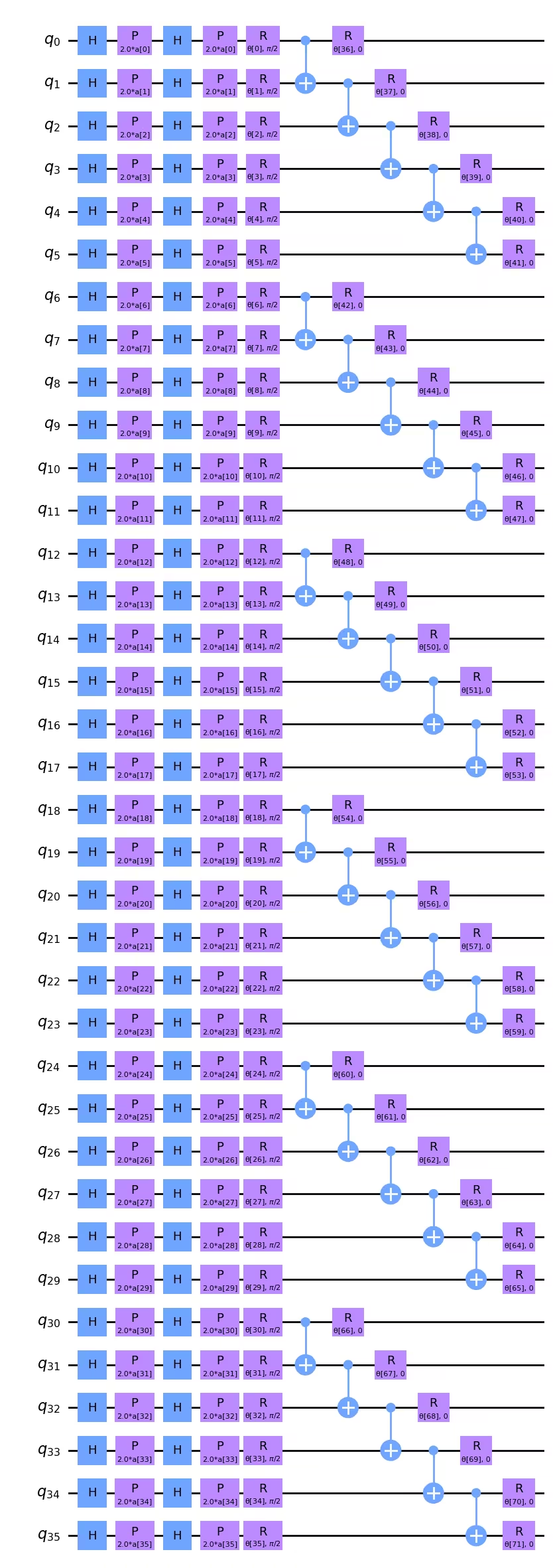
มาเริ่มต้นด้วยการขยายขนาดภาพ ไม่มีอะไรพิเศษเกี่ยวกับการเลือก grid 6x6 ยกเว้นว่ามันเกินจำนวน Qubit (32) ที่เราสามารถจำลองสำหรับ Circuit ที่ใช้ non-Clifford gates

```python
# This code defines the images to be classified:

import numpy as np

# Total number of "pixels"/qubits
size = 36
# One dimension of the image (called vertical, but it doesn't matter). Must be a divisor of `size`
vert_size = 6
# The length of the line to be detected (yellow). Must be less than or equal to the smallest dimension of the image (`<=min(vert_size,size/vert_size)`
line_size = 6

def generate_dataset(num_images):
    images = []
    labels = []
    hor_array = np.zeros((size - (line_size - 1) * vert_size, size))
    ver_array = np.zeros((round(size / vert_size) * (vert_size - line_size + 1), size))

    j = 0
    for i in range(0, size - 1):
        if i % (size / vert_size) <= (size / vert_size) - line_size:
            for p in range(0, line_size):
                hor_array[j][i + p] = np.pi / 2
            j += 1

    # Make two adjacent entries pi/2, then move down to the next row. Careful to avoid the "pixels" at size/vert_size - linesize, because we want to fold this list into a grid.

    j = 0
    for i in range(0, round(size / vert_size) * (vert_size - line_size + 1)):
        for p in range(0, line_size):
            ver_array[j][i + p * round(size / vert_size)] = np.pi / 2
        j += 1

    # Make entries pi/2, spaced by the length/rows, so that when folded, the entries appear on top of each other.

    for n in range(num_images):
        rng = np.random.randint(0, 2)
        if rng == 0:
            labels.append(-1)
            random_image = np.random.randint(0, len(hor_array))
            images.append(np.array(hor_array[random_image]))
            # Randomly select one of the several rows you made above.
        elif rng == 1:
            labels.append(1)
            random_image = np.random.randint(0, len(ver_array))
            images.append(np.array(ver_array[random_image]))
            # Randomly select one of the several rows you made above.

        # Create noise
        for i in range(size):
            if images[-1][i] == 0:
                images[-1][i] = np.random.rand() * np.pi / 4
    return images, labels

hor_size = round(size / vert_size)

เนื่องจากเวลาบนคอมพิวเตอร์ควอนตัมเป็นทรัพยากรอันมีค่า เราจะใช้ชุดข้อมูลการฝึกที่เล็กมาก และขั้นตอนการปรับให้เหมาะสมน้อยมาก สิ่งนี้เพียงพอที่จะสาธิตขั้นตอนการทำงาน

from sklearn.model_selection import train_test_split

np.random.seed(42)
# Here we specify a very small data set. Increase for realism, but monitor use of quantum computing time.
images, labels = generate_dataset(10)

train_images, test_images, train_labels, test_labels = train_test_split(
    images, labels, test_size=0.3, random_state=246
)

import matplotlib.pyplot as plt

# Generate a figure with nested images using subplots.

fig, ax = plt.subplots(2, 2, figsize=(10, 6), subplot_kw={"xticks": [], "yticks": []})
for i in range(4):
    ax[i // 2, i % 2].imshow(
        train_images[i].reshape(vert_size, hor_size),
        aspect="equal",
    )
plt.subplots_adjust(wspace=0.1, hspace=0.025)

Output of the previous code cell

ขั้นตอนที่ 1: แมปปัญหาเป็น Circuit ควอนตัม

from qiskit.circuit.library import z_feature_map

# One qubit per data feature
num_qubits = len(train_images[0])

# Data encoding
# Note that qiskit orders parameters alphabetically. We assign the parameter prefix "a" to ensure our data encoding goes to the first part of the circuit, the feature mapping.
feature_map = z_feature_map(num_qubits, parameter_prefix="a")

# This creates a circuit with the cxs in the compressed order.

from qiskit import QuantumCircuit
from qiskit.circuit import ParameterVector

qnn_circuit = QuantumCircuit(size)
params = ParameterVector("θ", length=2 * size)
for i in range(size):
    qnn_circuit.ry(params[i], i)

# CNOT gates between horizontally adjacent qubits.
for i in range(vert_size):
    for j in range(hor_size):
        if j < hor_size - 1:
            qnn_circuit.cx((i * hor_size) + j, (i * hor_size) + j + 1)

# CNOT gates between vertically adjacent qubits, likely not necessary based on our preliminary simulation.
#        if i<vert_size-1:
#            qnn_circuit.cx((i*hor_size)+j,(i*hor_size)+j+hor_size)
for i in range(size):
    qnn_circuit.rx(params[size + i], i)
qnn_circuit_large = qnn_circuit

print(qnn_circuit_large.decompose().depth())
print(
    f"2+ qubit depth: {qnn_circuit_large.decompose().depth(lambda instr: len(instr.qubits) > 1)}"
)
# qnn_circuit_large.draw()

7
2+ qubit depth: 5

นี่คือความลึก two-qubit ที่สมเหตุสมผล เราควรสามารถได้ผลลัพธ์คุณภาพสูงจากคอมพิวเตอร์ควอนตัมจริงได้

# Combine the feature map and variational circuit
ansatz = qnn_circuit

# Combine the feature map with the ansatz
full_circuit = QuantumCircuit(num_qubits)
full_circuit.compose(feature_map, range(num_qubits), inplace=True)
full_circuit.compose(ansatz, range(num_qubits), inplace=True)

# Check the depth of the full circuit
print(full_circuit.decompose().depth())
print(
    f"2+ qubit depth: {full_circuit.decompose().depth(lambda instr: len(instr.qubits) > 1)}"
)

11
2+ qubit depth: 5

เนื่องจากเราใช้ z_feature_map ซึ่งไม่มี CNOT gates การเพิ่มเลเยอร์การเข้ารหัสไม่ได้เพิ่มความลึก two-qubit เราสามารถแสดงภาพ Circuit เต็มรูปแบบได้ที่นี่

full_circuit.decompose().draw("mpl", style="clifford", idle_wires=False, fold=-1)

Output of the previous code cell

คุณอาจสังเกตว่าหากการลดความลึก two-qubit มีความสำคัญสูงสุด เราจริงๆ สามารถลดได้เล็กน้อยโดยเปลี่ยนลำดับของ CNOT ตัวอย่างเช่น CNOT บน $q_{35}$ และ $q_{34}$ สามารถย้ายไปทางซ้ายในแผนภาพ Circuit ด้านบน และสามารถวางไว้โดยตรงด้านล่าง CNOT บน $q_{30}$ และ $q_{31}$ ได้ สำหรับความลึก two-qubit gate ที่ 5 ไม่ชัดเจนว่าสิ่งนี้จะสร้างความแตกต่างหลังการ transpilation แต่เป็นสิ่งที่ควรคำนึงถึง ถ้าลำดับของ CNOT gates มีความสำคัญสำหรับการจับคู่ปัญหาในเชิงตรรกะ ความลึกที่นี่ก็ดีแล้ว ถ้าลำดับของ CNOT ไม่ได้สำคัญต่อการสร้างแบบจำลองโครงสร้างข้อมูลในภาพ เราสามารถเขียนสคริปต์เพื่อจัดเรียง CNOT gates ใหม่เพื่อลดความลึก

นอกจากนี้ เราต้องกำหนด observable ใหม่สำหรับภาพขนาดใหญ่ของเรา:

from qiskit.quantum_info import SparsePauliOp

observable = SparsePauliOp.from_list([("Z" * (num_qubits), 1)])

Qiskit Patterns ขั้นตอนที่ 2: ปรับปัญหาให้เหมาะสมสำหรับการประมวลผลควอนตัม

from qiskit_ibm_runtime import QiskitRuntimeService

# To run on hardware, select the least busy quantum computer or specify a particular one.
service = QiskitRuntimeService()
backend = service.least_busy(operational=True, simulator=False)
# backend = service.backend("ibm_brisbaneane")

print(backend.name)

ibm_brisbane

อีกครั้ง เรากำหนด pass manager โดยตั้งระดับ optimization เป็น 3

from qiskit.circuit.library import XGate
from qiskit.transpiler import PassManager
from qiskit.transpiler.passes import (
    ALAPScheduleAnalysis,
    ConstrainedReschedule,
    PadDynamicalDecoupling,
)
from qiskit.transpiler.preset_passmanagers import generate_preset_pass_manager

target = backend.target

pm = generate_preset_pass_manager(target=target, optimization_level=3)
pm.scheduling = PassManager(
    [
        ALAPScheduleAnalysis(target=target),
        ConstrainedReschedule(
            acquire_alignment=target.acquire_alignment,
            pulse_alignment=target.pulse_alignment,
            target=target,
        ),
        PadDynamicalDecoupling(
            target=target,
            dd_sequence=[XGate(), XGate()],
            pulse_alignment=target.pulse_alignment,
        ),
    ]
)

ตอนนี้เราจะใช้ pass manager หลายครั้ง สำหรับ Circuit ที่กว้างหรือลึกมาก อาจมีความแปรปรวนขนาดใหญ่ในความลึก two-qubit transpiled สำหรับ Circuit เช่นนั้น สิ่งสำคัญคือต้องลอง pass manager หลายครั้งและใช้ผลลัพธ์ที่ดีที่สุด (ตื้นที่สุด)

# Try pass manager several times, since heuristics can return various transpilations on large circuits, and we want the shallowest.

transpiled_qcs = []
transpiled_depths = []
transpiled_2q_depths = []
for i in range(1, 10):
    circuit_ibm = pm.run(full_circuit)
    transpiled_qcs.append(circuit_ibm)
    transpiled_depths.append(circuit_ibm.decompose().depth())
    transpiled_2q_depths.append(
        circuit_ibm.decompose().depth(lambda instr: len(instr.qubits) > 1)
    )
    # print(i)

print(transpiled_depths)
print(transpiled_2q_depths)

# Use the shallowest

minpos = transpiled_2q_depths.index(min(transpiled_2q_depths))

[85, 85, 81, 89, 81, 81, 89, 85, 85]
[10, 10, 10, 10, 10, 10, 10, 10, 10]

เราเห็นว่าในกรณีนี้ ความลึก two-qubit transpiled อยู่ที่ 10 เสมอ มีความแปรปรวนเล็กน้อยในความลึก single-qubit และเราจะใช้ Circuit ที่ตื้นที่สุด แต่สำหรับ Circuit 36 Qubit นี้ ไม่ใช่การปรับปรุงที่สำคัญ เราสามารถแสดงภาพ Circuit transpiled นี้ได้ แม้ว่าในระดับนี้จะยิ่งยากต่อการตีความทางสายตา

circuit_ibm = transpiled_qcs[2]
observable_ibm = observable.apply_layout(circuit_ibm.layout)
print(circuit_ibm.decompose().depth())
print(
    f"2+ qubit depth: {circuit_ibm.decompose().depth(lambda instr: len(instr.qubits) > 1)}"
)

81
2+ qubit depth: 10

Qiskit Patterns ขั้นตอนที่ 3: ประมวลผลโดยใช้ Qiskit Primitives

เพื่อจำกัดเวลาที่ใช้บนคอมพิวเตอร์ควอนตัมจริง เราจะทำขั้นตอนการปรับให้เหมาะสมเพียงไม่กี่ขั้นตอน และทำงานกับชุดข้อมูลการฝึกที่เล็กมาก แต่การขยายสิ่งนี้ไปยังขั้นตอนการปรับให้เหมาะสมมากขึ้นและชุดข้อมูลทดสอบที่ใหญ่ขึ้นควรชัดเจนจากคำแนะนำตลอดบทเรียน

# This was run on an Eagle r3 processor on 10-4-24, and took 7 min.

from qiskit_ibm_runtime import EstimatorV2 as Estimator, Session

batch_size = 7
num_epochs = 1
num_samples = len(train_images)

# Globals
circuit = circuit_ibm
observable = observable_ibm
objective_func_vals = []
iter = 0

# Random initial weights for the ansatz
np.random.seed(42)
# weight_params = np.random.rand(len(ansatz.parameters)) * 2 * np.pi
# Or re-load weights from a previous calculation
weight_params = np.array(
    [
        3.35330497,
        5.97351416,
        4.59925358,
        3.76148219,
        0.98029403,
        0.98014248,
        0.3649501,
        6.44234523,
        3.77691701,
        4.44895122,
        0.12933619,
        6.09412333,
        5.23039137,
        1.33416598,
        1.14243996,
        1.15236452,
        1.91161039,
        3.2971419,
        3.71399059,
        1.82984665,
        3.84438512,
        0.87646578,
        1.83559896,
        2.30191935,
        2.86557222,
        4.93340606,
        1.25458737,
        3.23103027,
        3.72225051,
        0.29185655,
        3.81731689,
        1.07143467,
        0.40873121,
        5.96202367,
        6.067245,
        5.07931034,
        1.91394476,
        0.61369199,
        4.2991629,
        2.76555968,
        0.76678884,
        3.11128829,
        0.21606945,
        5.71342859,
        1.62596258,
        4.16275028,
        1.95853845,
        3.26768375,
        3.43508199,
        1.1614748,
        6.09207989,
        4.87030317,
        5.90304595,
        5.62236606,
        3.75671636,
        5.79230665,
        0.55601479,
        1.23139664,
        0.28417144,
        2.04411075,
        2.44213144,
        1.70493625,
        5.20711134,
        2.24154726,
        1.76516358,
        3.40986006,
        0.88545302,
        5.04035228,
        0.46841551,
        6.2007935,
        4.85215699,
        1.24856745,
    ]
)

# Running in a session avoids repeated queuing. This is available to Premium Plan, Flex Plan, and On-Prem (IBM Quantum Platform API) Plan users.

with Session(backend=backend) as session:
    estimator = Estimator(mode=session, options={"resilience_level": 1})

    for epoch in range(num_epochs):
        for i in range((num_samples - 1) // batch_size + 1):
            print(f"Epoch: {epoch}, batch: {i}")
            start_i = i * batch_size
            end_i = start_i + batch_size
            train_images_batch = np.array(train_images[start_i:end_i])
            train_labels_batch = np.array(train_labels[start_i:end_i])
            input_params = train_images_batch
            target = train_labels_batch
            iter = 0
            # We can increase maxiter to do a full optimization.
            res = minimize(
                mse_loss_weights,
                weight_params,
                method="COBYLA",
                options={"maxiter": 20},
            )
            weight_params = res["x"]
session.close()

# Open users can carry out the same calculation using a batch, but repeated queuing is possible.
# from qiskit_ibm_runtime import Batch

# with Batch(backend=backend) as batch:
#    estimator = Estimator(
#        mode=batch, options={"resilience_level": 1}
#    )
#
#    for epoch in range(num_epochs):
#        for i in range((num_samples - 1) // batch_size + 1):
#            print(f"Epoch: {epoch}, batch: {i}")
#            start_i = i * batch_size
#            end_i = start_i + batch_size
#            train_images_batch = np.array(train_images[start_i:end_i])
#            train_labels_batch = np.array(train_labels[start_i:end_i])
#            input_params = train_images_batch
#            target = train_labels_batch
#            iter = 0
#            # We can increase maxiter to do a full optimization.
#            res = minimize(
#                mse_loss_weights,
#                weight_params,
#                method="COBYLA",
#                options={"maxiter": 20},
#            )
#            weight_params = res["x"]
# batch.close()

แนะนำให้บันทึกพารามิเตอร์ weight ที่ได้จากการคำนวณนี้ ในกรณีที่คุณต้องการทำซ้ำต่อไป

weight_params

array([3.35330497, 6.97351416, 5.59925358, 3.76148219, 0.98029403,
       0.98014248, 0.3649501 , 6.44234523, 3.77691701, 4.44895122,
       1.12933619, 7.09412333, 5.23039137, 1.33416598, 1.14243996,
       1.15236452, 1.91161039, 3.2971419 , 3.71399059, 1.82984665,
       3.84438512, 0.87646578, 1.83559896, 2.30191935, 2.86557222,
       4.93340606, 1.25458737, 3.23103027, 3.72225051, 0.29185655,
       3.81731689, 1.07143467, 0.40873121, 5.96202367, 6.067245  ,
       5.07931034, 1.91394476, 0.61369199, 4.2991629 , 2.76555968,
       0.76678884, 3.11128829, 0.21606945, 5.71342859, 1.62596258,
       4.16275028, 1.95853845, 3.26768375, 3.43508199, 1.1614748 ,
       6.09207989, 4.87030317, 5.90304595, 5.62236606, 3.75671636,
       5.79230665, 0.55601479, 1.23139664, 0.28417144, 2.04411075,
       2.44213144, 1.70493625, 5.20711134, 2.24154726, 1.76516358,
       3.40986006, 0.88545302, 5.04035228, 0.46841551, 6.2007935 ,
       4.85215699, 1.24856745])

เราสามารถพล็อตขั้นตอนการปรับให้เหมาะสมแรกเหล่านี้ แม้ว่าเราจะไม่คาดหวัง convergence หลังจากเพียงไม่กี่ขั้นตอนการปรับให้เหมาะสม curve เหล่านี้ค่อนข้างราบสำหรับขั้นตอนแรกๆ แม้ใช้ซิมูเลเตอร์ อย่างไรก็ตาม ควรทราบว่าการปรับให้เหมาะสมในปัจจุบันมีพารามิเตอร์อิสระ 72 ตัว ซึ่งสามารถลดได้อย่างน้อย 2-3 เท่าโดยไม่กระทบผลลัพธ์ โดยตัวอย่างเช่น การกำหนดพารามิเตอร์ให้กับ Qubit ที่มีข้อมูลสอดคล้องกับแถวและคอลัมน์ย่อย จริงๆ ควรลดพื้นที่พารามิเตอร์ก่อนที่จะใช้เวลาบนคอมพิวเตอร์ควอนตัมมากขึ้นในการลด loss function

obj_func_vals_qc = objective_func_vals
# import matplotlib.pyplot as plt

plt.figure(figsize=(12, 6))
plt.plot(obj_func_vals_qc, label="revised ansatz")
plt.xlabel("iteration")
plt.ylabel("loss")
plt.legend()
plt.show()

Output of the previous code cell

สรุป

สรุป ในบทเรียนนี้เราได้เรียนรู้ขั้นตอนการทำงานสำหรับการจำแนกประเภทไบนารีของภาพโดยใช้ quantum neural network การพิจารณาหลักในแต่ละขั้นตอน Qiskit patterns ได้แก่:

ขั้นตอนที่ 1: แมปปัญหาเป็น Circuit ควอนตัม

โหลดข้อมูลการฝึก ซึ่งสามารถทำ "โดยตรง" หรือใช้แผนที่ฟีเจอร์สำเร็จรูปอย่าง z_feature_map
สร้าง ansatz ที่มีเลเยอร์การหมุนและ entanglement ที่เหมาะสมกับปัญหาของคุณ
ติดตามความลึกของ Circuit เพื่อให้ได้ผลลัพธ์ที่มีคุณภาพบนคอมพิวเตอร์ควอนตัม

ขั้นตอนที่ 2: ปรับปัญหาให้เหมาะสมสำหรับการประมวลผลควอนตัม

เลือก Backend มักเป็นตัวที่ว่างที่สุด
ใช้ pass manager เพื่อ transpile ทั้ง Circuit และ observables ให้เข้ากับสถาปัตยกรรมของ Backend ที่เลือก
สำหรับ Circuit ที่ลึกหรือกว้างมาก ให้ transpile หลายครั้งและเลือก Circuit ที่ตื้นที่สุด

ขั้นตอนที่ 3: ประมวลผลโดยใช้ Qiskit (Runtime) Primitives

ทดลองเบื้องต้นบนซิมูเลเตอร์เพื่อ debug และปรับ ansatz
ประมวลผลบนคอมพิวเตอร์ควอนตัมของ IBM®

ขั้นตอนที่ 4: ประมวลผลหลังการวัด คืนผลลัพธ์ในรูปแบบคลาสสิก

คำนวณความแม่นยำของโมเดลบนข้อมูลการฝึก และบนข้อมูลทดสอบ
ติดตาม convergence ของการปรับให้เหมาะสมแบบคลาสสิก

อ้างอิง

[1] https://arxiv.org/abs/2405.00781

Source: IBM Quantum docs — updated 15 ม.ค. 2569

English version on doQumentation — updated 7 พ.ค. 2569

This translation based on the English version of approx. 26 มี.ค. 2569

การสร้างข้อมูล​

Variational quantum classifier: ความพยายามแรก​

Qiskit patterns ขั้นตอนที่ 1: แมปปัญหาเป็น Circuit ควอนตัม​

Loss function​

Qiskit Patterns ขั้นตอนที่ 2: ปรับปัญหาให้เหมาะสมสำหรับการประมวลผลควอนตัม​

Qiskit Patterns ขั้นตอนที่ 3: ประมวลผลโดยใช้ Qiskit Primitives​

วนซ้ำชุดข้อมูลเป็น batch และ epoch​

Qiskit Patterns ขั้นตอนที่ 4: ประมวลผลหลังการวัด คืนผลลัพธ์ในรูปแบบคลาสสิก​

การทดสอบและความแม่นยำ​

การปรับปรุงโมเดล​

ทบทวนขั้นตอนที่ 1​

ทบทวนขั้นตอนที่ 2​

ทบทวนขั้นตอนที่ 3​

ทบทวนขั้นตอนที่ 4​

ขั้นตอนที่ 1: แมปปัญหาเป็น Circuit ควอนตัม​

Qiskit Patterns ขั้นตอนที่ 2: ปรับปัญหาให้เหมาะสมสำหรับการประมวลผลควอนตัม​

Qiskit Patterns ขั้นตอนที่ 3: ประมวลผลโดยใช้ Qiskit Primitives​

สรุป​

อ้างอิง​

การสร้างข้อมูล

Variational quantum classifier: ความพยายามแรก

Qiskit patterns ขั้นตอนที่ 1: แมปปัญหาเป็น Circuit ควอนตัม

Loss function

Qiskit Patterns ขั้นตอนที่ 2: ปรับปัญหาให้เหมาะสมสำหรับการประมวลผลควอนตัม

Qiskit Patterns ขั้นตอนที่ 3: ประมวลผลโดยใช้ Qiskit Primitives

วนซ้ำชุดข้อมูลเป็น batch และ epoch

Qiskit Patterns ขั้นตอนที่ 4: ประมวลผลหลังการวัด คืนผลลัพธ์ในรูปแบบคลาสสิก

การทดสอบและความแม่นยำ

การปรับปรุงโมเดล

ทบทวนขั้นตอนที่ 1

ทบทวนขั้นตอนที่ 2

ทบทวนขั้นตอนที่ 3

ทบทวนขั้นตอนที่ 4

ขั้นตอนที่ 1: แมปปัญหาเป็น Circuit ควอนตัม

Qiskit Patterns ขั้นตอนที่ 2: ปรับปัญหาให้เหมาะสมสำหรับการประมวลผลควอนตัม

Qiskit Patterns ขั้นตอนที่ 3: ประมวลผลโดยใช้ Qiskit Primitives

สรุป

อ้างอิง