Postselection ด้วยการตรวจสอบความผิดพลาดแบบ non-Markovian

คู่มือนี้อธิบายว่าการตรวจสอบความผิดพลาดแบบ non-Markovian คืออะไรและวิธีนำไปใช้ในซอฟต์แวร์ด้วย qiskit-mitigation คุณจะเริ่มจากตัวอย่างขนาดเล็กสอง qubit เพื่อดูภาพของการตรวจสอบและพูดคุยถึงวิธีการทำงาน หลังจากที่คุณเริ่มมีความเข้าใจเชิงสัญชาตญาณแล้ว คุณจะลองตัวอย่าง 20 qubit ที่คุณนำการตรวจสอบไปใช้และเปรียบเทียบกลยุทธ์ postselection ต่างๆ

การตรวจสอบความผิดพลาดแบบ non-Markovian คืออะไร

การตรวจสอบความผิดพลาดแบบ non-Markovian คือการทดสอบด้วยการวัดว่าสถานะของ qubit น่าจะถูกทำให้เสียหายจากแหล่งความผิดพลาดแบบ non-Markovian หรือไม่ การทดสอบนี้ทำโดยวาง gate พลิกบิตที่มีระยะเวลายาวขึ้น (xslow หรืออนุกรมของ gate rx จำนวน $N$ ตัวที่มีมุม $\frac{\pi}{N}$) บน qubit แต่ละตัวที่จุดเริ่มต้นของ circuit ตามด้วย XGate ปกติ แล้ววัดเพื่อให้แน่ใจว่าสถานะพลิกสำเร็จจาก $|0\rangle \mapsto |1\rangle \mapsto |0\rangle$ การทดสอบนี้ยังทำได้ที่ท้าย circuit หลังการวัดสุดท้ายแต่ละครั้ง เพื่อให้แน่ใจว่าอุปกรณ์พลิกสถานะที่วัดได้ของ qubit จาก $|x\rangle \mapsto |x\oplus1\rangle$ ได้สำเร็จ ตัวอย่างที่เกี่ยวข้องกับการตรวจสอบที่ไม่ผ่านอาจถือว่าเชื่อถือไม่ได้ และการทำ postselection เฉพาะตัวอย่างที่ผ่านการตรวจสอบทั้งหมดสามารถเพิ่ม fidelity ของการแจกแจงที่มีสัญญาณรบกวนได้

กลยุทธ์การทำ postselection จากการตรวจสอบความผิดพลาดแบบ non-Markovian

• Postselection แบบอิงโหนด: เลือกเฉพาะตัวอย่างที่ qubit ทุกตัวผ่านการตรวจสอบของมัน นี่เป็นกลยุทธ์ที่เข้มงวดที่สุด และโดยทั่วไปทำให้ตัวอย่างถูกทิ้งมากกว่า

• Postselection แบบอิงเส้นเชื่อม: สำหรับแต่ละเส้นเชื่อมในกราฟการเชื่อมต่อของ qubit ให้แน่ใจว่ามี qubit อย่างน้อยหนึ่งตัวผ่านการตรวจสอบ กลยุทธ์นี้ผ่อนปรนกว่า: หาก qubit ตัวหนึ่งตรวจสอบไม่ผ่าน ตัวอย่างนั้นก็ยังอาจถูกเก็บไว้หากเพื่อนบ้านทั้งหมดของมันผ่านการตรวจสอบ

Spectator qubit

คุณสามารถระบุ qubit ช่วย "spectator" ที่อยู่ติดกับ qubit ซึ่งใช้รัน circuit ต้นฉบับได้ การตรวจสอบความผิดพลาดแบบ non-Markovian สามารถวางบน spectator เหล่านี้ ซึ่งให้ความครอบคลุมต่อสัญญาณรบกวนแบบ non-Markovian ที่การตรวจสอบเหล่านี้ออกแบบมาตรวจจับมากขึ้น

ส่วนที่ 1 แสดงภาพการตรวจสอบความผิดพลาดแบบ non-Markovian

ก่อนสาธิตเทคนิคนี้บน QPU คุณจะสร้าง circuit ขนาดเล็กสอง qubit และเพิ่มการตรวจสอบเพื่อดูภาพว่ามันทำงานอย่างไร เริ่มจากสถานะ Bell ที่ transpile ไปยัง QPU backend ibm_kingston

# Added by doQumentation — installs the packages this notebook needs if they are missing
import importlib.util

_needed = {"matplotlib": "matplotlib", "numpy": "numpy", "qiskit": "qiskit", "qiskit_ibm_runtime": "qiskit-ibm-runtime", "qiskit_mitigation": "qiskit-mitigation", "samplomatic": "samplomatic"}
_missing = [pip for module, pip in _needed.items()
            if importlib.util.find_spec(module) is None]
# One at a time, so a package that fails to install does not block the others
for _pip in _missing:
    %pip install -q {_pip}
if not _missing:
    print("\u2713 All required packages are installed")

from qiskit import QuantumCircuit
from qiskit.transpiler import generate_preset_pass_manager
from qiskit_ibm_runtime import QiskitRuntimeService

service = QiskitRuntimeService(channel="ibm_quantum_platform")
backend = service.backend("ibm_kingston")

qc = QuantumCircuit(2)
qc.h(0)
qc.cx(0, 1)
qc.measure_all()
qc_isa = generate_preset_pass_manager(
    optimization_level=0, backend=backend
).run(qc)
qc_isa.draw("mpl")

เพิ่มการตรวจสอบความผิดพลาดแบบ non-Markovian บางส่วนที่จุดเริ่มต้นของ circuit การตรวจสอบจะถูกวางเฉพาะบน qubit ที่ลงท้ายด้วยการวัด การตรวจสอบเหล่านี้ช่วยให้แน่ใจว่าอุปกรณ์พลิกสถานะเริ่มต้นของ qubit จาก $|0\rangle \mapsto |1\rangle \mapsto |0\rangle$ ได้สำเร็จ และผลการวัดของการตรวจสอบเหล่านี้ถูกอ่านออกในรีจิสเตอร์คลาสสิกใหม่ชื่อ meas_pre

from qiskit.transpiler import PassManager
from qiskit_mitigation.postselection.passes import (
    AddPreCircuitNonMarkovianErrorChecks,
)

qc_w_checks = PassManager([AddPreCircuitNonMarkovianErrorChecks()]).run(
    qc_isa
)
qc_w_checks.draw("mpl", idle_wires=False)

ในทำนองเดียวกัน คุณสามารถเพิ่มการตรวจสอบที่ท้าย circuit หลังการวัดสุดท้ายแต่ละครั้งได้ การตรวจสอบเหล่านี้ช่วยให้แน่ใจว่าอุปกรณ์พลิกสถานะของ qubit จาก $|x\rangle \mapsto |x\oplus1\rangle$ ได้ และผลการวัดของมันถูกอ่านออกในรีจิสเตอร์คลาสสิกใหม่ชื่อ meas_ps

from qiskit_mitigation.postselection.passes import (
    AddPostCircuitNonMarkovianErrorChecks,
)

qc_w_checks = PassManager([AddPostCircuitNonMarkovianErrorChecks()]).run(
    qc_w_checks
)
qc_w_checks.draw("mpl", idle_wires=False)

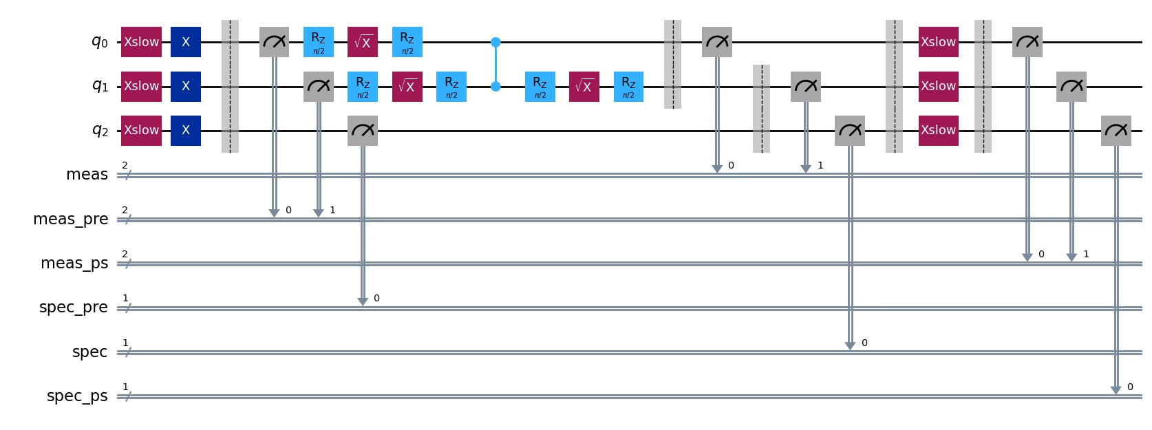
ตามที่กล่าวไว้ในบทนำ คุณสามารถใช้ ancilla qubit ที่อยู่ติดกับ data qubit เป็น "ผู้สังเกตการณ์" (spectator) เพื่อให้ครอบคลุมข้อผิดพลาดได้มากขึ้น เพิ่มการตรวจสอบ spectator ก่อน circuit และหลัง circuit คุณจะเห็นว่าเนื่องจาก physical qubit 2 บน ibm_kingston อยู่ติดกับ data qubit 1 จึงถูกเพิ่มเป็น spectator และมีการเพิ่มการตรวจสอบก่อนและหลัง circuit ให้กับมัน ผลการวัดของ spectator ถูกเพิ่มลงใน classical register ใหม่ที่ชื่อ spec_pre และ spec

Circuit แบบนี้มีการตรวจสอบข้อผิดพลาดแบบ non-Markovian ที่เป็นไปได้ทั้งหมด ดังนั้นการสุ่มตัวอย่างจาก circuit นี้ทำให้ผู้ใช้สามารถทำ postselection ตามการตรวจสอบ [ก่อน/หลัง] circuit และกลยุทธ์ postselection แบบ [node/edge] ได้ทุกแบบรวมกัน ดูส่วนที่ 2 ของคู่มือนี้เพื่อดูว่าทำงานบนฮาร์ดแวร์ควอนตัมอย่างไร

from qiskit_mitigation.postselection.passes import (
    AddSpectatorPostCircuitNonMarkovianErrorChecks,
    AddSpectatorPreCircuitNonMarkovianErrorChecks,
)

qc_w_checks = PassManager(
    [
        AddSpectatorPreCircuitNonMarkovianErrorChecks(
            coupling_map=backend.coupling_map
        ),
        AddSpectatorPostCircuitNonMarkovianErrorChecks(
            coupling_map=backend.coupling_map
        ),
    ]
).run(qc_w_checks)
qc_w_checks.draw("mpl", idle_wires=False, fold=-1)

ส่วนที่ 2: สาธิตการตรวจสอบข้อผิดพลาดแบบ non-Markovian บน QPU และเปรียบเทียบกลยุทธ์ postselection

ตอนนี้คุณเข้าใจแล้วว่าการตรวจสอบข้อผิดพลาดแบบ non-Markovian คืออะไรและถูกนำไปใช้ในซอฟต์แวร์อย่างไร คุณจึงสามารถรันตัวอย่างที่ใหญ่ขึ้นบน QPU และดูว่ามันทำงานอย่างไร ขั้นแรก เตรียม circuit การเลือก circuit ไม่ใช่เรื่องสำคัญมากนัก ขอเพียงเป็น circuit ที่ตรวจสอบผลลัพธ์ได้ง่าย ที่นี่เราเลือก mirrored Ising circuit แบบ 1 มิติ 20 qubit circuit นี้รันบนฮาร์ดแวร์ได้ไม่ง่าย และควรได้รับผลกระทบจากข้อผิดพลาดแบบ non-Markovian ซึ่งเปิดโอกาสให้สาธิตประสิทธิภาพของการตรวจสอบข้อผิดพลาดแบบ non-Markovian นอกจากนี้ โครงสร้างแบบ mirrored ยังช่วยให้เราเปรียบเทียบค่าคาดหมายที่มีสัญญาณรบกวนกับค่าที่แน่นอนได้อย่างตรงไปตรงมา

ในการทดลองนี้ เรากำลังคำนวณค่าคาดหมายของ observable การเลือก observable $O$ ก็ไม่สำคัญเช่นกัน เราจึงเลือกค่าแมกนีไทเซชันต่อไซต์เฉลี่ย $O=\frac{1}{N}\sum_i\langle Z_i\rangle$ แบบง่ายๆ

import numpy as np
from qiskit.quantum_info import SparsePauliOp
from qiskit.transpiler import CouplingMap

num_qubits = 20
initial_layout = initial_layout = [
    124,
    125,
    126,
    127,
    128,
    129,
    130,
    131,
    132,
    133,
    134,
    135,
    139,
    155,
    154,
    153,
    152,
    151,
    150,
    149,
][:num_qubits]
coupling_map = CouplingMap.from_line(num_qubits, bidirectional=False)

# Num Trotter steps and `rx` angle
num_steps = 6
theta_rx = np.pi / 6

# Average single-site magnetization
observable = (
    SparsePauliOp(
        [
            "I" * iq + "Z" + "I" * (num_qubits - iq - 1)
            for iq in range(num_qubits)
        ]
    )
    / num_qubits
)

# Create the Trotter circuit
circuit = QuantumCircuit(num_qubits)
edges = CouplingMap.from_line(num_qubits, bidirectional=False).get_edges()
edges_a = [e for e in edges if e[0] % 2 == 0]
edges_b = [e for e in edges if e[0] % 2 == 1]
for _ in range(num_steps):
    circuit.rx(theta_rx, [i for i in range(num_qubits)])
    for edge in edges_a:
        circuit.cz(edge[0], edge[1])
    for edge in edges_b:
        circuit.cz(edge[0], edge[1])
circuit = circuit.compose(circuit.inverse())
circuit.measure_all()

# Transpile circuit to backend
pm = generate_preset_pass_manager(
    optimization_level=0, backend=backend, initial_layout=initial_layout
)
isa_circuit = pm.run(circuit)
print(
    f"two-qubit depth: {isa_circuit.depth(lambda instr: instr.operation.num_qubits == 2)}"
)
print(f"total depth:     {isa_circuit.depth()}")
isa_circuit.draw("mpl", fold=-1, idle_wires=False)

two-qubit depth: 24
total depth:     85

ตอนนี้เราเพิ่มการตรวจสอบก่อนและหลัง circuit บนทุก qubit รวมถึง spectator qubit ที่อยู่ติดกันทั้งเจ็ดตัว เมื่อคุณเพิ่มการตรวจสอบที่เป็นไปได้ทั้งหมดลงใน circuit คุณสามารถตัดสินใจได้ว่าจะใช้กลยุทธ์ postselection แบบไหนในขั้นตอนประมวลผลภายหลัง

# Use all non-Markovian error checks so we can compare all strategies in post-processing.
combined = PassManager(
    [
        AddPreCircuitNonMarkovianErrorChecks(x_pulse_type="rx"),
        AddSpectatorPreCircuitNonMarkovianErrorChecks(
            backend.coupling_map, x_pulse_type="rx"
        ),
        AddPostCircuitNonMarkovianErrorChecks(x_pulse_type="rx"),
        AddSpectatorPostCircuitNonMarkovianErrorChecks(
            backend.coupling_map, x_pulse_type="rx"
        ),
    ]
).run(isa_circuit)
combined_isa = generate_preset_pass_manager(
    optimization_level=0, backend=backend
).run(combined)

print("cregs:", [(c.name, c.size) for c in combined_isa.cregs])

cregs: [('meas', 20), ('meas_pre', 20), ('spec_pre', 7), ('meas_ps', 20), ('spec', 7), ('spec_ps', 7)]

ใช้ primitive Executor เพื่อสุ่มตัวอย่าง circuit ที่มีการตรวจสอบ

from qiskit_ibm_runtime import Executor
from samplomatic.quantum_program import QuantumProgram

# Raw and combined-checks circuits in a single 100k-shot program so they share calibration.
program = QuantumProgram(shots=100_000)
program.append_circuit_item(isa_circuit)  # raw circuit, no checks
program.append_circuit_item(
    combined_isa
)  # combined pre + post non-Markovian error checks
job = Executor(backend).run(program)
print(f"job id: {job.job_id()}")
print(f"status: {job.status()}")

job id: d9badrm6hjac73ffe31g
status: QUEUED

คลาส PostSelector รู้จักโครงสร้าง creg ของการตรวจสอบ จึงสามารถเชื่อมโยงแต่ละบิตในตัวอย่างกับการวัดใน circuit ที่เกี่ยวข้องได้ เมธอด compute_mask ของมันใช้สร้าง mask เหนือลำดับของตัวอย่าง โดยกำหนดกลยุทธ์ postselection (node หรือ edge) และประเภทของการตรวจสอบข้อผิดพลาดแบบ non-Markovian ที่จะดู (ก่อนหรือหลัง circuit) หากต้องการรวมกลยุทธ์ก่อนและหลัง circuit เป็น mask เดียว สามารถคำนวณ mask แยกกันแล้วรวมด้วยการดำเนินการ AND ที่นี่เราใช้ PostSelector สร้าง mask สำหรับทุกกลยุทธ์ แล้วดูผลลัพธ์จากทุกการจัดกลุ่มของกลยุทธ์ที่มี

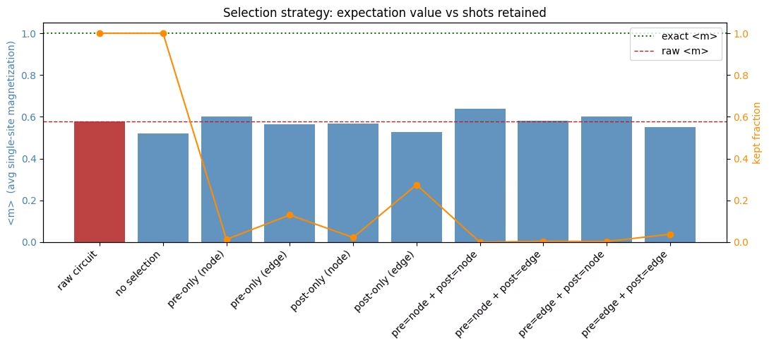
ในภาพแสดงผลด้านล่าง เราจะเห็นว่ากลยุทธ์ postselection ส่งผลต่ออัตรา postselection และคุณภาพของคำตอบอย่างไร ตามที่คาดไว้ กลยุทธ์ที่ใช้ postselection แบบ node ให้อัตรา postselection ต่ำที่สุด กลยุทธ์แบบ edge ผ่อนปรนกว่าและมักให้อัตรา postselection สูงกว่า ผู้ใช้ควรทดลองกลยุทธ์ต่างๆ กับปัญหาของตนเพื่อหาสมดุลที่เหมาะสมระหว่างอัตรา postselection และคุณภาพของการแจกแจงตัวอย่าง ในตัวอย่างนี้ การใช้ postselection แบบ node กับการตรวจสอบก่อนและหลัง circuit ให้คำตอบที่ดีที่สุดด้วยอัตรา postselection ที่ .028% บางกลยุทธ์ไม่ได้ดีกว่า circuit ดิบ คุณจะเห็นด้วยว่าการเพิ่มการตรวจสอบแต่ไม่ใช้เลย (แท่งที่มีป้าย "no selection" ในแผนภูมิด้านล่าง) ให้ผลแย่ที่สุด

import matplotlib.pyplot as plt
from qiskit_mitigation.postselection import PostSelector

selector = PostSelector.from_circuit(combined_isa, backend.coupling_map)

exec_results = job.result()
# The Executor returns numpy arrays keyed by classical-register name, so each result item is
# already the {creg_name: ndarray} mapping that compute_mask expects.
raw_bits = exec_results[0]["meas"]  # raw circuit, no checks
bits = exec_results[1]  # combined pre+post circuit

meas_bits = bits["meas"]
total = meas_bits[..., 0].size

def magnetization(b, mask=None):
    """Average single-site magnetization over the (optionally masked) measurement bits."""
    kept = b if mask is None else b[mask]
    return (1 - 2 * kept.astype(int)).mean()  # bit 0 -> +1, bit 1 -> -1

rows = []

def report(label, mask=None, b=meas_bits):
    """Record and print the magnetization and kept fraction for one selection strategy."""
    kept = b[..., 0].size if mask is None else int(mask.sum())
    ev = magnetization(b, mask)
    rows.append((label, ev, kept / total))
    print(f"{label:<24}: <m> = {ev:+.4f}   (kept {kept:>6}/{total})")

# Compare all possible postselection strategies
report("raw circuit", b=raw_bits)
report("no selection")
for s in ("node", "edge"):
    report(f"pre-only ({s})", selector.compute_mask(bits, s, mode="pre"))
for s in ("node", "edge"):
    report(f"post-only ({s})", selector.compute_mask(bits, s, mode="post"))
for pre_s in ("node", "edge"):
    for post_s in ("node", "edge"):
        keep = selector.compute_mask(
            bits, pre_s, mode="pre"
        ) & selector.compute_mask(bits, post_s, mode="post")
        report(f"pre={pre_s} + post={post_s}", keep)

labels = [r[0] for r in rows]
evs = [r[1] for r in rows]
fracs = [r[2] for r in rows]
x = range(len(labels))

fig, ax1 = plt.subplots(figsize=(11, 5))

# Bars: expectation value per selection strategy.
bar_colors = ["firebrick"] + ["steelblue"] * (len(evs) - 1)
ax1.bar(x, evs, color=bar_colors, alpha=0.85)
ax1.axhline(1.0, color="green", ls=":", lw=1.5, label="exact <m>")
ax1.axhline(rows[0][1], color="firebrick", ls="--", lw=1, label="raw <m>")
ax1.set_ylabel("<m>  (avg single-site magnetization)", color="steelblue")
ax1.tick_params(axis="y", labelcolor="steelblue")
ax1.set_xticks(list(x))
ax1.set_xticklabels(labels, rotation=45, ha="right")
ax1.legend(loc="upper right")

# Line: fraction of shots retained (right axis).
ax2 = ax1.twinx()
ax2.plot(x, fracs, "o-", color="darkorange")
ax2.set_ylabel("kept fraction", color="darkorange")
ax2.tick_params(axis="y", labelcolor="darkorange")
ax2.set_ylim(0, 1.05)

ax1.set_title("Selection strategy: expectation value vs shots retained")
fig.tight_layout()
plt.show()

raw circuit             : <m> = +0.5791   (kept 100000/100000)
no selection            : <m> = +0.5211   (kept 100000/100000)
pre-only (node)         : <m> = +0.6026   (kept   1357/100000)
pre-only (edge)         : <m> = +0.5637   (kept  13029/100000)
post-only (node)        : <m> = +0.5682   (kept   2254/100000)
post-only (edge)        : <m> = +0.5265   (kept  27514/100000)
pre=node + post=node    : <m> = +0.6393   (kept     28/100000)
pre=node + post=edge    : <m> = +0.5799   (kept    442/100000)
pre=edge + post=node    : <m> = +0.6006   (kept    317/100000)
pre=edge + post=edge    : <m> = +0.5521   (kept   3836/100000)