Zero-noise extrapolation ด้วย gate folding และการ extrapolate แบบกำหนดเอง

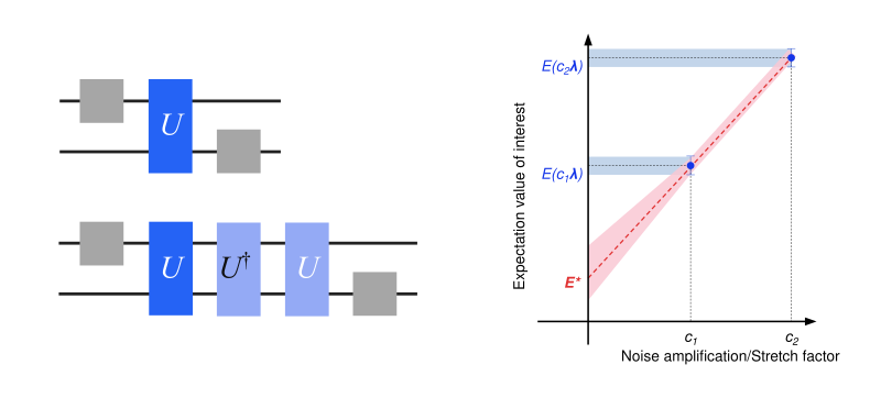
Zero-noise extrapolation (ZNE) เป็นเทคนิคลดสัญญาณรบกวนควอนตัมในการคำนวณค่าคาดหวังของ observable ทำงานโดยรัน quantum circuit ที่ระดับสัญญาณรบกวนเพิ่มขึ้น หาค่าคาดหวังที่ระดับสัญญาณรบกวนเหล่านั้น แล้ว extrapolate เพื่อประมาณค่าคาดหวังที่ไม่มีสัญญาณรบกวน ทั้งขั้นตอนการขยายสัญญาณรบกวนและการ extrapolate ทำได้หลายวิธี คู่มือนี้ขยายสัญญาณรบกวนด้วย "digital gate folding" ซึ่งหมายถึงการแทนที่ two-qubit gate ด้วยลำดับที่เทียบเท่าของ gate และอินเวอร์สของมัน ตัวอย่างเช่น การแทนที่ unitary $U$ ด้วย $U U^† U$ จะให้ตัวประกอบการขยายสัญญาณรบกวนเท่ากับ 3 คุณยังขยายด้วย probabilistic error amplification (PEA) ได้ ซึ่งต้องมีขั้นตอนเพิ่มเติมคือการเรียนรู้โมเดลสัญญาณรบกวน และกล่าวถึงไว้ในคู่มือ probabilistic error amplification คู่มือนี้ extrapolate ด้วยกลยุทธ์การ fit ที่มีมาให้สองแบบ (เชิงเส้นและเอกซ์โพเนนเชียล) และยังสาธิตวิธี implement ฟังก์ชัน fit แบบกำหนดเองด้วย

โปรดจำไว้ว่า แม้ ZNE จะลดสัญญาณรบกวนควอนตัมได้ผลด้วยต้นทุนการสุ่มตัวอย่างต่ำกว่าวิธีอื่น แต่ก็ไม่มีขอบเขตรับประกันสำหรับ bias

ขั้นตอนการทำงานมีดังนี้:

1. ระบุ circuit และ observable
2. คำนวณค่าคาดหวังที่แน่นอนโดยใช้ตัวจำลอง statevector ของ Qiskit
3. คำนวณค่าคาดหวังที่มีสัญญาณรบกวนและยังไม่ลดสัญญาณรบกวน
4. เตรียมโปรแกรม ZNE ด้วย digital gate folding และสุ่มตัวอย่าง circuit ที่ระดับสัญญาณรบกวนต่าง ๆ
5. Extrapolate ไปยังลิมิตที่ไม่มีสัญญาณรบกวนด้วยฟังก์ชัน fit ที่มีมาให้และแบบกำหนดเอง
6. เปรียบเทียบค่าคาดหวังที่ลดสัญญาณรบกวนแล้ว

ระบุ circuit และ observable

คำนวณแมกนีไทเซชันเฉลี่ยตามตำแหน่ง $\langle Z \rangle_{\text{avg}} = \frac{1}{N} \sum_{i=1}^{N} \langle Z_i \rangle$ ของแบบจำลอง Ising สนามขวาง (TFIM) แบบ Trotter บนแปด qubit ในโทโพโลยีวงแหวน คุณจะกวาดค่าความแรงของสนามขวางหลายค่าและพล็อตแมกนีไทเซชันเป็นฟังก์ชันของความแรงสนาม

# Added by doQumentation — installs the packages this notebook needs if they are missing
import importlib.util

_needed = {"IPython": "IPython", "matplotlib": "matplotlib", "numpy": "numpy", "qiskit": "qiskit", "qiskit_aer": "qiskit-aer", "qiskit_ibm_runtime": "qiskit-ibm-runtime", "qiskit_mitigation": "qiskit-mitigation", "scipy": "scipy"}
_missing = [pip for module, pip in _needed.items()
            if importlib.util.find_spec(module) is None]
# One at a time, so a package that fails to install does not block the others
for _pip in _missing:
    %pip install -q {_pip}
if not _missing:
    print("\u2713 All required packages are installed")

import warnings

import numpy as np
from qiskit.circuit import Parameter, QuantumCircuit
from qiskit.quantum_info import SparsePauliOp

warnings.filterwarnings("ignore")

def trotter_circuit(num_qubits, theta, layers, num_steps):
    """Trotterized transverse-field Ising evolution: RX on every site, then a CZ layer per coupling layer."""
    circuit = QuantumCircuit(num_qubits)
    for _ in range(num_steps):
        circuit.rx(theta, range(num_qubits))
        for layer in layers:
            circuit.barrier()
            for edge in layer:
                circuit.cz(*edge)
                circuit.sdg(edge)
            circuit.barrier()
    return circuit

num_qubits = 8
trotter_steps = 15
ring_coupling = [(i, (i + 1) % num_qubits) for i in range(num_qubits)]
layers = [
    ring_coupling[0::2],
    ring_coupling[1::2],
]  # two disjoint layers of CZ gates
theta = Parameter("theta")
circuit = trotter_circuit(num_qubits, theta, layers, trotter_steps)

# Parameter values: theta in [0, 0.25 pi] - values for the transverse-field sweep
data_points = 6
parameter_values = np.linspace(0, 0.25 * np.pi, data_points).reshape(
    (data_points, 1)
)

# Define observables - Z on each site
observables = [
    SparsePauliOp("I" * (num_qubits - q - 1) + "Z" + "I" * q)
    for q in range(num_qubits)
]

print("Visualization of 1 Trotter step")
trotter_circuit(num_qubits, theta, layers, 1).draw("mpl", scale=0.7)

Visualization of 1 Trotter step

คำนวณค่าคาดหวังที่แน่นอนโดยใช้ตัวจำลอง statevector ของ Qiskit

ใช้คลาส Statevector ของ Qiskit เพื่อคำนวณค่าคาดหวังที่แน่นอนของ $Z_i$ ที่แต่ละตำแหน่งสำหรับทุกค่าของ $\theta$

import matplotlib.pyplot as plt
from qiskit.quantum_info import Statevector

exact_evs = np.array(
    [
        [
            Statevector(circuit.assign_parameters([value]))
            .expectation_value(obs)
            .real
            for value in parameter_values.ravel()
        ]
        for obs in observables
    ]
)  # shape (observables, parameter values)

x_vals = parameter_values.ravel() / np.pi
fig, ax = plt.subplots(figsize=(7, 4))
ax.plot(x_vals, exact_evs.mean(axis=0), "ko-", label="Exact")
ax.set_xlabel(r"$\theta/\pi$")
ax.set_ylabel(r"$\langle Z \rangle_{\text{avg}}$")
ax.legend()
plt.tight_layout()
plt.show()

คำนวณค่าคาดหวังที่มีสัญญาณรบกวนและยังไม่ลดสัญญาณรบกวน

QuantumProgram ประกอบด้วย quantum circuit และ samplex ในรูปแบบที่เหมาะกับ Executor primitive MitigationTask.prepare สร้าง QuantumProgram จาก circuit, observable และค่าพารามิเตอร์ และใส่ box ให้ circuit ตามตัวเลือก boxing ที่กำหนด คุณตั้งตัวเลือก boxing measure_annotations เป็น "change_basis" ซึ่งหมุนการวัดไปยังฐานที่ต้องการ และเพิ่ม add_tags: "unique_box" เพื่อให้ตัวจำลองแมปโมเดลสัญญาณรบกวนลงบน box ของ circuit ได้ โปรแกรมจะถูก Pauli-twirl โดยค่าเริ่มต้น ซึ่งบนฮาร์ดแวร์จะเปลี่ยนสัญญาณรบกวนแบบ coherent ให้เป็นสัญญาณรบกวนแบบ Pauli ที่วิธีลดสัญญาณรบกวนสมมติไว้ num_randomizations กำหนดจำนวนอินสแตนซ์ที่ถูก twirl ของแต่ละ circuit ที่สุ่มตัวอย่าง และ shots_per_randomization กำหนดจำนวน shot ที่แต่ละอินสแตนซ์ได้รับ ผลคูณของทั้งสองจึงเป็นงบ shot ต่อ circuit

ผู้ใช้ที่เข้าถึง QPU ได้จะรันโปรแกรมด้วย Executor ที่สร้างจาก Backend ของ QiskitRuntimeService ในที่นี้ คุณจะส่ง AerSimulator ให้ Executor ซึ่งรันโปรแกรมในเครื่อง และใช้ตัวเลือกตัวจำลอง layer_noise_model เพื่อฉีดโมเดลสัญญาณรบกวน Pauli-Lindblad แบบสุ่มลงในทุกเลเยอร์ของ entangling gate ที่สร้างด้วย random_pauli_lindblad_noise จาก qiskit-mitigation โดยมี error per layered gate (EPLG) เท่ากับ 0.003 ซึ่งเป็นค่าทั่วไปของ QPU Heron ในปัจจุบัน

from qiskit.circuit import CircuitInstruction
from qiskit.quantum_info import PauliLindbladMap, pauli_basis
from qiskit_aer import AerSimulator
from qiskit_ibm_runtime import Executor
from qiskit_mitigation import MitigationTask, find_combined_unique_layers

def generate_random_pauli_lindblad_noise(
    layers,
    num_qubits: int,
    eplg: float = 3e-3,
    seed: int | None = None,
) -> list[tuple[CircuitInstruction, PauliLindbladMap]]:
    """Generate random Pauli-Lindblad noise over the full Pauli basis."""
    layer_noise_model = []
    for layer in layers:
        layer_instructions = layer.operation.params[0]
        contain_measurement = any(
            inst.name.startswith("measure") for inst in layer_instructions
        )
        if contain_measurement:  # do not add measurement noise
            layer_noise = PauliLindbladMap.identity(num_qubits)
        else:
            edges = [
                (inst.qubits[0]._index, inst.qubits[1]._index)
                for inst in layer_instructions
            ]  # extract the edges of the layer

            basis_paulis = [p for p in pauli_basis(2) if np.sum(p.x + p.z)]
            rng = np.random.default_rng(seed=seed)
            num_generators = len(basis_paulis)
            rates = rng.random(len(basis_paulis)) * eplg / num_generators

            layer_noise = PauliLindbladMap.from_sparse_list(
                [
                    (pauli.to_label(), edge, rate)
                    for pauli, rate in zip(basis_paulis, rates, strict=True)
                    for edge in edges
                ],
                num_qubits=num_qubits,
            )
        layer_noise_model.append((layer, layer_noise))
    return layer_noise_model

num_randomizations = 50
shots_per_randomization = 64

boxing_options = {
    "measure_annotations": "change_basis",
    "add_tags": "unique_box",
}

# find the unique layers to generate the layered noise for
box_layers = find_combined_unique_layers(
    [circuit], custom_boxing_options=boxing_options
)
layer_noise_model = generate_random_pauli_lindblad_noise(
    box_layers, num_qubits, seed=42
)

# a local noisy simulator in place of a QPU backend
noisy_executor = Executor(
    AerSimulator(),
    options={"simulator": {"layer_noise_model": layer_noise_model}},
)

task = MitigationTask()
program = task.prepare(
    circuit=circuit,
    observables=observables,
    parameters=parameter_values,
    num_randomizations=num_randomizations,
    shots_per_randomization=shots_per_randomization,
    custom_boxing_options=boxing_options,
)
program._semantic_role = "simulation"  # flag the program for the simulator
unmitigated_res = task.postprocess(noisy_executor.run(program).result())

fig, ax = plt.subplots(figsize=(7, 4))
ax.plot(x_vals, exact_evs.mean(axis=0), "k-", label="Exact")
ax.errorbar(
    x_vals,
    np.mean(unmitigated_res.data.evs, axis=0),
    np.mean(unmitigated_res.data.stds, axis=0),
    fmt="o-",
    label="Unmitigated",
)
ax.set_xlabel(r"$\theta/\pi$")
ax.set_ylabel(r"$\langle Z \rangle_{\text{avg}}$")
ax.legend()
plt.tight_layout()
plt.show()

เตรียมโปรแกรม ZNE ด้วย digital gate folding และสุ่มตัวอย่าง circuit ที่ระดับสัญญาณรบกวนต่าง ๆ

เตรียมโปรแกรม ZNE ที่มี circuit ซึ่งมีระดับสัญญาณรบกวนเพิ่มขึ้น แต่ละ noise factor แทนจำนวนเท่าของ entangling gate ที่ circuit มี (noise factor 3.0 มี entangling gate มากกว่า circuit ดั้งเดิมสามเท่า) circuit ของแต่ละ noise factor ถูก twirl ด้วยจำนวน randomization และ shot เท่ากับโปรแกรมที่ยังไม่ลดสัญญาณรบกวน

from qiskit_mitigation import GateFolding

task_gf = GateFolding()
program_zne = task_gf.prepare(
    circuit=circuit,
    observables=observables,
    parameters=parameter_values,
    num_randomizations=num_randomizations,
    shots_per_randomization=shots_per_randomization,
    custom_boxing_options=boxing_options,
    noise_factors=[1, 3, 5],  # ZNE option
)

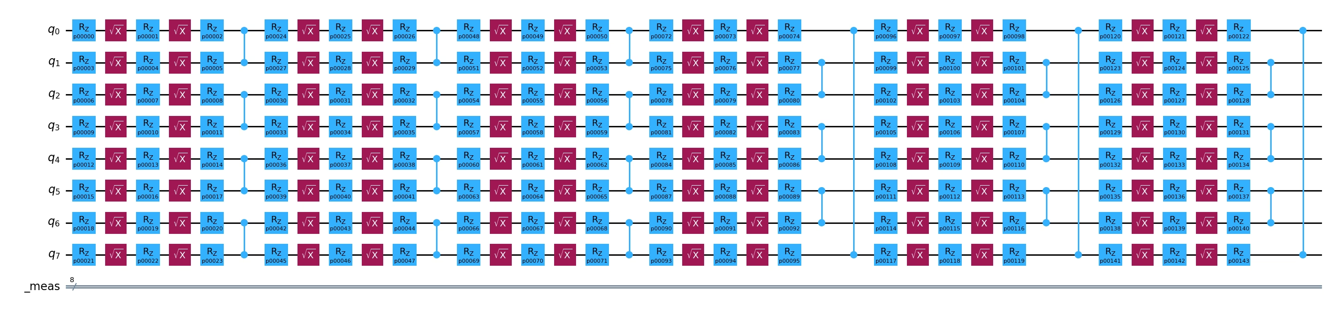
วาด Trotter step แรกของ template ที่ถูก twirl ด้วย noise factor 1 และ noise factor 3 เพื่อดูภาพการขยาย สำหรับ noise factor 3.0 ทุกเลเยอร์ของ circuit จะถูกแทนที่ด้วยเลเยอร์ อินเวอร์สของมัน และเลเยอร์อีกครั้ง

import IPython.display

def first_trotter_step(template, noise_factor):
    """The template up to the closing barrier of its first Trotter step (two layers, each folded ``noise_factor`` times)."""
    toy = template.copy_empty_like()
    for instruction in template.data:
        toy.append(instruction)
        if (
            instruction.operation.name == "barrier"
            and instruction.operation.label.startswith(
                f"R{2 * noise_factor - 1}@"
            )
        ):
            break
    return toy

IPython.display.display(
    first_trotter_step(program_zne.items[0].circuit, 1).draw(
        "mpl", scale=0.7, plot_barriers=False
    )
)
first_trotter_step(program_zne.items[1].circuit, 3).draw(
    "mpl", fold=-1, plot_barriers=False
)

สุดท้าย รันโปรแกรมบนตัวจำลองที่มีสัญญาณรบกวน ผลลัพธ์จะถูกนำไปใช้ในการ extrapolate ในขั้นตอนถัดไป

program_zne._semantic_role = (
    "simulation"  # flag the program for the simulator
)
job_zne_results = noisy_executor.run(program_zne).result()

Extrapolate ไปยังลิมิตที่ไม่มีสัญญาณรบกวนด้วยฟังก์ชัน fit ที่มีมาให้และแบบกำหนดเอง

เมื่อคุณมีข้อมูลสำหรับแต่ละระดับสัญญาณรบกวนแล้ว คุณสามารถ fit ฟังก์ชันกับข้อมูลและ extrapolate กลับไปยังค่าที่ไม่มีสัญญาณรบกวนเพื่อประมาณค่าคาดหวังของ observable ที่ไร้สัญญาณรบกวน มีหลายวิธีในการ fit ข้อมูล และฟังก์ชันที่เหมาะสมขึ้นกับลักษณะของข้อมูลที่สุ่มตัวอย่าง GateFolding.postprocess มีฟังก์ชัน extrapolate ในตัวหลายแบบ รวมถึง linear, exponential และ double_exponential เมธอด postprocess รับรายการวิธี extrapolate ประเมินตามลำดับ และคืนค่าแรกที่มีค่าถูกต้องทางฟิสิกส์และความแปรปรวนจำกัด นั่นหมายความว่าลำดับที่คุณระบุ extrapolator มีผลมากต่อการเลือก extrapolator การส่ง fallback เป็น extrapolator หมายความว่าหากไม่พบคำตอบที่ถูกต้อง จะเลือกและคืนค่าคาดหวังของ noise factor ที่เล็กที่สุด หากไม่ส่ง fallback และไม่มี extrapolator ใดให้ค่าที่ถูกต้องทางฟิสิกส์ จะคืนผลลัพธ์ที่มี std เล็กที่สุด ภายใต้สัญญาณรบกวนแบบ Pauli observable จะสลายแบบเอกซ์โพเนนเชียลตาม noise factor ดังนั้นเมื่อมี 30 เลเยอร์ (15 Trotter step, 2 เลเยอร์ต่อ step) ของ entangling gate extrapolator แบบเอกซ์โพเนนเชียลจึงเป็นตัวเลือกที่เป็นธรรมชาติ คุณยัง extrapolate แบบเชิงเส้นได้ ซึ่งเป็นตัวเลือกทั่วไปเมื่อการสลายมีค่าน้อย

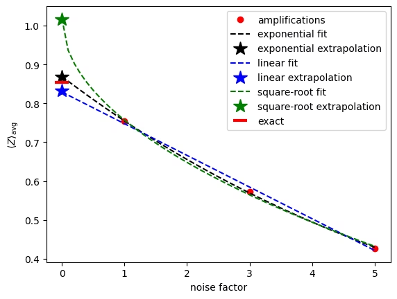
หากต้องการใช้ฟังก์ชัน fit แบบกำหนดเอง ให้ส่ง extrapolator "custom" พร้อม tuple custom_fit ที่ประกอบด้วยฟังก์ชัน fit รายการค่าเริ่มต้นโดยประมาณของแต่ละพารามิเตอร์ และขอบเขต ค่าเหล่านี้จะถูกส่งต่อไปยัง scipy.optimize.curve_fit การประมวลผลภายหลังทำซ้ำได้ด้วย extrapolator อื่นโดยไม่ต้องรันโปรแกรมใหม่ ในที่นี้คุณใช้ฟังก์ชัน fit แบบรากที่สองแบบกำหนดเอง เพื่อแสดงภาพการ extrapolate ให้พล็อตแมกนีไทเซชันเฉลี่ยตามตำแหน่งที่คำนวณที่แต่ละ noise factor สำหรับ $\theta = 0.15\pi$ เส้น fit ทั้งสามแบบ และค่าเฉลี่ยตามตำแหน่งของค่าคาดหวังที่ extrapolate ที่จุดไร้สัญญาณรบกวน จุดข้อมูลทั้งสามดูเกือบเป็นเส้นตรง แต่การ extrapolate เชิงเส้นตกลงต่ำกว่าค่าที่แน่นอนอย่างเห็นได้ชัด ตามที่คาดไว้ การ fit แบบเอกซ์โพเนนเชียลประมาณค่าคาดหวังที่ไร้สัญญาณรบกวนได้ดีที่สุด

from scipy.optimize import curve_fit

zne_mitigated_exp = task_gf.postprocess(
    job_zne_results, extrapolator=["exponential", "linear"]
)
zne_mitigated_lin = task_gf.postprocess(
    job_zne_results, extrapolator=["linear"]
)

def sqrt_fit(x, a, b):
    return a * np.sqrt(x) + b

custom_fit = (sqrt_fit, [1.0, 1.0], (-np.inf, np.inf))
zne_mitigated_custom = task_gf.postprocess(
    job_zne_results,
    extrapolator=["custom", "exponential", "linear"],
    custom_fit=custom_fit,
)

# The result holds the expectation value at each noise factor and the extrapolated value, but
# not the fit parameters, so we refit the same models here to draw the curves.
noise_factors = np.array([1, 3, 5])
angle = 3  # theta = 0.15 pi, the angle with the largest unmitigated error
amplifications = zne_mitigated_exp.data.evs_noise_factors[:, angle, :].mean(
    axis=0
)
x_fit = np.linspace(0, 5, 51)
fits = {
    "exponential": (
        lambda x, a, b: a * np.exp(b * x),
        zne_mitigated_exp,
        "black",
    ),
    "linear": (lambda x, a, b: a * x + b, zne_mitigated_lin, "blue"),
    "square-root": (sqrt_fit, zne_mitigated_custom, "green"),
}

plt.plot(
    noise_factors, amplifications, "o", color="red", label="amplifications"
)
for name, (fit, res, color) in fits.items():
    params, _ = curve_fit(fit, noise_factors, amplifications, p0=[1.0, -0.1])
    plt.plot(
        x_fit, fit(x_fit, *params), "--", color=color, label=f"{name} fit"
    )
    plt.plot(
        [0],
        res.data.evs[:, angle].mean(),
        "*",
        color=color,
        markersize=15,
        label=f"{name} extrapolation",
    )
plt.plot(
    [0],
    exact_evs[:, angle].mean(),
    "_",
    color="red",
    markersize=15,
    markeredgewidth=3,
    label="exact",
)
plt.xlabel("noise factor")
plt.ylabel(r"$\langle Z \rangle_{\text{avg}}$")
plt.legend()
plt.show()

เปรียบเทียบค่าคาดหวังที่ลดสัญญาณรบกวนแล้ว

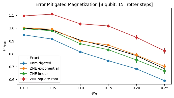
พล็อตแมกนีไทเซชันเฉลี่ยตามตำแหน่งของแต่ละวิธีตลอดการกวาดมุมหมุน Ising การ extrapolate แบบเอกซ์โพเนนเชียลกู้คืนแมกนีไทเซชันที่แน่นอนได้ภายในแท่งความคลาดเคลื่อน ขณะที่การ extrapolate เชิงเส้นลบ bias ได้มากแต่ต่ำกว่าค่าจริงอย่างสม่ำเสมอ เพราะการสลายที่แท้จริงเป็นแบบเอกซ์โพเนนเชียล ส่วนการ fit แบบรากที่สองเกินค่าจริงไปมาก

results = {
    "Unmitigated": unmitigated_res,
    "ZNE exponential": zne_mitigated_exp,
    "ZNE linear": zne_mitigated_lin,
    "ZNE square-root": zne_mitigated_custom,
}

fig, ax = plt.subplots(figsize=(7, 4))
ax.plot(x_vals, exact_evs.mean(axis=0), "k-", label="Exact")
for label, res in results.items():
    ax.errorbar(
        x_vals,
        np.mean(res.data.evs, axis=0),
        np.mean(res.data.stds, axis=0),
        fmt="o-",
        label=label,
    )
ax.set_xlabel(r"$\theta/\pi$")
ax.set_ylabel(r"$\langle Z \rangle_{\text{avg}}$")
ax.legend()
ax.set_title(
    f"Error-Mitigated Magnetization [{num_qubits}-qubit, {trotter_steps} Trotter steps]"
)
plt.tight_layout()
plt.show()