PEC ร่วมกับ SLC

Probabilistic error cancellation (PEC) เป็นเทคนิคลดสัญญาณรบกวนควอนตัมในการคำนวณค่าคาดหมายของ observable ช่วยให้คุณคำนวณค่าประมาณของค่าคาดหมายที่ไม่เอนเอียงได้ เทคนิคนี้ทำงานโดยรันชุดของ circuit ที่มีสัญญาณรบกวนซึ่งถูกฉีดด้วยอินเวอร์สของโมเดลสัญญาณรบกวนที่เรียนรู้ได้ จากนั้นโมเดลสัญญาณรบกวนจะถูกประมาณเป็นช่องสัญญาณ Pauli ด้วยการทำ Pauli twirling (หรือเรียกว่า randomized compiling) โมเดลสัญญาณรบกวนแบบนี้เรียนรู้ได้อย่างมีประสิทธิภาพ และลดสัญญาณรบกวนได้ด้วย PEC (ดูรายละเอียดเพิ่มเติมใน Probabilistic error cancellation with sparse Pauli-Lindblad models on noisy quantum processors)

PEC ต้องใช้โอเวอร์เฮดของ shot แบบเอกซ์โพเนนเชียลเพื่อคำนวณค่าประมาณที่ไม่เอนเอียง Shaded Lightcones (SLC) เป็นเทคนิคที่ใช้ทรัพยากรคลาสสิกเพื่อกำหนดขอบเขตความไวต่อความผิดพลาดตลอดทั้ง circuit จากขอบเขตเหล่านี้ ผู้ใช้สามารถปรับอคติในการประมาณค่า observable ได้อย่างควบคุมได้

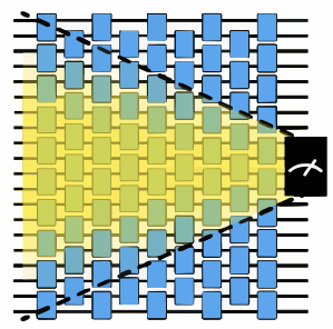
คู่มือนี้แสดงวิธีใช้ PEC ร่วมกับ SLC เพื่อลดสัญญาณรบกวนของ gate โดยมีโอเวอร์เฮดของ shot น้อยกว่า PEC แบบดั้งเดิม

ขั้นตอนการทำงานมีดังนี้:

1. กำหนด circuit และ observable
2. คำนวณค่าคาดหมายที่มีสัญญาณรบกวนและไม่ได้ลดสัญญาณรบกวน
3. คำนวณขอบเขตไปข้างหน้าและย้อนกลับของอคติ
4. เรียนรู้สัญญาณรบกวนของเลเยอร์ที่สร้างพันกันด้วย qiskit-noise-learning
5. ใช้สัญญาณรบกวนที่เรียนรู้ได้เพื่อรวมขอบเขตที่คำนวณไว้เป็นเมทริกซ์ local scales
6. เลือกขอบเขตอคติที่ต้องการโดยพิจารณาจากการแลกเปลี่ยนระหว่างโอเวอร์เฮดของ shot กับอคติ
7. เตรียมโปรแกรม PEC + SLC รันโปรแกรม และประมวลผลหลังการรัน
8. เปรียบเทียบค่าคาดหมายที่ลดสัญญาณรบกวนแล้วและโอเวอร์เฮดของ shot

กำหนด circuit และ observable

เตรียม mirror circuit ของการวิวัฒน์ตามเวลาแบบ Trotter ของ Hamiltonian โซ่ Ising 1 มิติบน qubit แปดตัว ทำ mirror ให้ circuit เพื่อหักล้างยูนิทารีของมันและได้ identity circuit ดังนั้นค่าคาดหมายในอุดมคติของแต่ละ observable จึงเป็น 1 โดยไม่ต้องคำนวณ นอกจากนี้ การทำ mirror ยังเพิ่มความลึกของ circuit เป็นสองเท่า ซึ่งทำให้ผลของสัญญาณรบกวนเพิ่มเป็นสองเท่าด้วย

ใช้มุม $\theta= \frac{\pi}{4}$ เพื่อให้พลวัตเป็นแบบไม่ใช่ Clifford

# Added by doQumentation — installs the packages this notebook needs if they are missing
import importlib.util

_needed = {"matplotlib": "matplotlib", "numpy": "numpy", "qiskit": "qiskit", "qiskit_addon_slc": "qiskit-addon-slc", "qiskit_aer": "qiskit-aer", "qiskit_ibm_runtime": "qiskit-ibm-runtime", "qiskit_mitigation": "qiskit-mitigation", "qiskit_noise_learning": "qiskit-noise-learning", "samplomatic": "samplomatic"}
_missing = [pip for module, pip in _needed.items()
            if importlib.util.find_spec(module) is None]
# One at a time, so a package that fails to install does not block the others
for _pip in _missing:
    %pip install -q {_pip}
if not _missing:
    print("\u2713 All required packages are installed")

import warnings

import numpy as np
from qiskit.circuit import QuantumCircuit
from qiskit.quantum_info import SparsePauliOp
from qiskit_mitigation.utils import get_measurement_bases

warnings.filterwarnings("ignore")

def construct_ising_circuit(
    num_qubits: int,
    num_trotter_steps: int,
    rx_angle: float,
) -> QuantumCircuit:
    circuit = QuantumCircuit(num_qubits)

    for _ in range(num_trotter_steps):
        circuit.rx(rx_angle, range(num_qubits))
        for first_qubit in (1, 2):
            for idx in range(first_qubit, num_qubits, 2):
                # equivalent to Rzz(-pi/2):
                circuit.sdg([idx - 1, idx])
                circuit.cz(idx - 1, idx)

    return circuit

def prepare_basis(
    circuit: QuantumCircuit, basis: list[int]
) -> QuantumCircuit:
    # basis is a list of integer values from 0 to 3. These map to the basis measurement as:
    # 0 = I; 1 = Z; 2 = X; 3 = Y
    assert len(basis) == circuit.num_qubits

    out_circ = circuit.copy_empty_like()
    for qb, bas in enumerate(basis):
        if bas == 2:
            out_circ.h(qb)
        elif bas == 3:
            out_circ.rx(-np.pi / 2, qb)

    out_circ.barrier()
    out_circ.compose(circuit, inplace=True)
    return out_circ

def mirror_circuit(circuit: QuantumCircuit) -> QuantumCircuit:
    mirror_circ = circuit.copy_empty_like()
    mirror_circ.compose(circuit.inverse(), inplace=True)
    mirror_circ.barrier()
    mirror_circ.compose(circuit, inplace=True)
    mirror_circ.measure_active()
    return mirror_circ

# define observables
num_qubits = 8  # Width of the Ising chain
# The observable to measure: one X component (on qubit 2) and one Z component (on qubit 5)
target_obs_sparse = [("XZ", [2, 5], 1.0)]
observable = SparsePauliOp.from_sparse_list(
    target_obs_sparse, num_qubits=num_qubits
)

# Determine the measurement basis each qubit requires for this observable.
bases, _ = get_measurement_bases(observable)

# Instantiate the mirrored circuit and prepend the basis-preparation gates
num_trotter_steps = 6
rx_angle = np.pi / 4
circuit = construct_ising_circuit(num_qubits, num_trotter_steps, rx_angle)
mirrored_circuit = mirror_circuit(circuit)
mirrored_circuit = prepare_basis(mirrored_circuit, bases[0])
print("Visualization of 1 mirrored Trotter step")
prepare_basis(
    mirror_circuit(construct_ising_circuit(num_qubits, 1, rx_angle)), bases[0]
).draw("mpl", scale=0.6, fold=-1)

Visualization of 1 mirrored Trotter step

คำนวณค่าคาดหมายที่มีสัญญาณรบกวนและไม่ได้ลดสัญญาณรบกวน

QuantumProgram ประกอบด้วย quantum circuit และ samplex ในรูปแบบที่เหมาะกับ primitive Executor MitigationTask.prepare สร้าง QuantumProgram จาก circuit, observable และค่าพารามิเตอร์ และครอบ circuit ด้วยกล่องตามตัวเลือก boxing ที่ระบุ ตั้งตัวเลือก boxing measure_annotations เป็น "change_basis" เพื่อหมุนการวัดไปยังฐานที่ต้องการ และเพิ่ม add_tags: "unique_box" เพื่อให้ซิมูเลเตอร์จับคู่โมเดลสัญญาณรบกวนกับกล่องของ circuit ได้ โดยค่าเริ่มต้นโปรแกรมจะถูกทำ Pauli twirl ซึ่งบนฮาร์ดแวร์จะเปลี่ยนสัญญาณรบกวนแบบ coherent ให้เป็นสัญญาณรบกวนแบบ Pauli ตามที่วิธีลดสัญญาณรบกวนสมมติไว้ num_randomizations กำหนดจำนวนอินสแตนซ์ที่ถูก twirl ของแต่ละ circuit ที่สุ่มตัวอย่าง และ shots_per_randomization กำหนดจำนวน shot ที่แต่ละอินสแตนซ์ได้รับ ผลคูณของสองค่านี้จึงเป็นขีดจำกัด shot ต่อ circuit

หากคุณเข้าถึง QPU ได้ คุณสามารถรันโปรแกรมด้วย Executor ที่สร้างจาก backend ของ QiskitRuntimeService ตัวอย่างนี้ใช้ AerSimulator เพื่อรันโปรแกรมในเครื่อง ตัวเลือกซิมูเลเตอร์ layer_noise_model ของมันฉีดสัญญาณรบกวนจากโมเดลสัญญาณรบกวน Pauli-Lindblad ที่กำหนดในทุกเลเยอร์ของ gate ที่สร้างพันกัน ตรงนี้เราสร้างโมเดลสัญญาณรบกวน Pauli-Lindblad แบบสุ่มที่มีค่าความผิดพลาดต่อ gate ในเลเยอร์ (EPLG) เท่ากับ 0.01 ซึ่งสูงกว่า QPU Heron ทั่วไปในปัจจุบันเกือบหนึ่งอันดับขนาด เพื่อขยายผลของการใช้ SLC แม้ในปัญหาขนาดเล็ก

from qiskit.circuit import CircuitInstruction
from qiskit.quantum_info import PauliLindbladMap, pauli_basis
from qiskit_aer import AerSimulator
from qiskit_ibm_runtime import Executor
from qiskit_mitigation import MitigationTask, find_combined_unique_layers
from samplomatic import Tag
from samplomatic.utils import get_annotation

def generate_random_pauli_lindblad_noise(
    layers,
    num_qubits: int,
    eplg: float = 3e-3,
    seed: int | None = None,
) -> list[tuple[CircuitInstruction, PauliLindbladMap]]:
    """Generate random Pauli-Lindblad noise over the full Pauli basis."""
    layer_noise_model = []
    for layer in layers:
        layer_instructions = layer.operation.params[0]
        contain_measurement = any(
            inst.name.startswith("measure") for inst in layer_instructions
        )
        if contain_measurement:  # do not add measurement noise
            layer_noise = PauliLindbladMap.identity(num_qubits)
        else:
            edges = [
                (inst.qubits[0]._index, inst.qubits[1]._index)
                for inst in layer_instructions
            ]  # extract the edges of the layer

            basis_paulis = [p for p in pauli_basis(2) if np.sum(p.x + p.z)]
            rng = np.random.default_rng(seed=seed)
            num_generators = len(basis_paulis)
            rates = rng.random(len(basis_paulis)) * eplg / num_generators

            layer_noise = PauliLindbladMap.from_sparse_list(
                [
                    (pauli.to_label(), edge, rate)
                    for pauli, rate in zip(basis_paulis, rates, strict=True)
                    for edge in edges
                ],
                num_qubits=num_qubits,
            )
        layer_noise_model.append((layer, layer_noise))
    return layer_noise_model

num_randomizations = 400
shots_per_randomization = 16

boxing_options = {"add_tags": "unique_box"}

# find the unique layers to generate the layered noise for
box_layers = find_combined_unique_layers(
    [mirrored_circuit], custom_boxing_options=boxing_options
)
layer_noise_model = generate_random_pauli_lindblad_noise(
    box_layers, num_qubits, eplg=1e-2, seed=42
)

# a local noisy simulator in place of a QPU backend
noisy_executor = Executor(
    AerSimulator(),
    options={"simulator": {"layer_noise_model": layer_noise_model}},
)

task = MitigationTask()
program = task.prepare(
    circuit=mirrored_circuit,
    observables=observable,
    parameters=None,
    num_randomizations=num_randomizations,
    shots_per_randomization=shots_per_randomization,
    custom_boxing_options=boxing_options,
)

program._semantic_role = "simulation"  # flag the program for the simulator
job_unmit_res = noisy_executor.run(program).result()
unmitigated_res = task.postprocess(job_unmit_res)

print(f"unmitigated result: {unmitigated_res.data.evs[0]}")

unmitigated result: 0.63125

คำนวณขอบเขตไปข้างหน้าและย้อนกลับของอคติ

ก่อนที่จะใช้เวลา QPU ไปกับการเรียนรู้สัญญาณรบกวน SLC ใช้การจำลองแบบคลาสสิกเพื่อกำหนดขอบเขตการมีส่วนต่ออคติของ observable จากความผิดพลาดที่อาจเกิดขึ้นแต่ละตัว ซึ่งทำใน 2 รอบที่เสริมกัน:

• การแพร่กระจายไปข้างหน้า: ความผิดพลาดแบบ Pauli แต่ละตัวถูกแพร่กระจายไปข้างหน้าผ่านส่วนที่เหลือของ circuit และประเมิน commutator ของมันกับ observable ความผิดพลาดที่ anti-commute กับ observable เป็นชนิดเดียวที่ทำให้ผลลัพธ์เอนเอียงได้ รอบนี้จึงให้ขอบเขตบนของผลกระทบไปข้างหน้าของความผิดพลาดแต่ละตัว

• การแพร่กระจายย้อนกลับ: ความผิดพลาดแต่ละตัวถูกแพร่กระจายย้อนกลับไปยังจุดเริ่มต้นของ circuit และประเมิน commutator ของมันกับสถานะเริ่มต้น เนื่องจาก circuit เริ่มจากสถานะศูนย์ทั้งหมด ความผิดพลาดที่ commute กับสถานะนี้จึงไม่ส่งผลต่อผลลัพธ์ ทำให้ขอบเขตแคบลงจากอีกทิศทางหนึ่ง

ขอบเขตทั้งสองรวมกันเป็นกรอบแคบๆ รอบการมีส่วนต่ออคติในกรณีเลวร้ายที่สุดของความผิดพลาดทุกตัว ในขั้นตอนถัดไป ขอบเขตเหล่านี้จะถูกรวมกับอัตราสัญญาณรบกวนที่เรียนรู้ได้ เพื่อจัดอันดับว่าความผิดพลาดใดควรแก้ไข และความผิดพลาดใดปล่อยไว้ได้อย่างปลอดภัย ต้องใช้ตัวเลือก boxing inject_noise_strategy="individual_modification" ตรงนี้ เพื่อให้แต่ละ annotation InjectNoise ใน circuit ที่ถูกครอบกล่องมีเอกลักษณ์เฉพาะที่ขอบเขต SLC สามารถผูกเข้าไปได้

สำหรับปัญหาขนาดใหญ่ขึ้น การคำนวณเหล่านี้อาจต้องใช้ทรัพยากรการคำนวณแบบคลาสสิกจำนวนมาก

from qiskit_addon_slc.bounds import (
    compute_backward_bounds,
    compute_forward_bounds,
    tighten_with_speed_limit,
)
from qiskit_mitigation import PEC

slc_boxing_options = {
    "add_tags": "unique_box",
    "inject_noise_strategy": "individual_modification",
}

slc_pec_task = PEC()

boxed_circuit, noise_model_paulis = (
    slc_pec_task.generate_slc_bounds_computation_input(
        mirrored_circuit, custom_boxing_options=slc_boxing_options
    )
)

forward_bounds = compute_forward_bounds(
    boxed_circuit, noise_model_paulis, observable
)
tighten_forward_bounds = tighten_with_speed_limit(
    forward_bounds, boxed_circuit, noise_model_paulis, observable
)
backward_bounds = compute_backward_bounds(boxed_circuit, noise_model_paulis)

เรียนรู้สัญญาณรบกวนของเลเยอร์ที่สร้างพันกัน

เพื่อคำนวณค่าประมาณสุดท้ายว่าความผิดพลาดแต่ละตัวส่งผลต่ออคติของค่าคาดหมายมากเพียงใด และการแก้ไขจะมีค่าใช้จ่ายเท่าไร เราเรียนรู้อัตราสัญญาณรบกวนแล้วนำไปใช้กับขอบเขตสัญญาณรบกวนที่คาดการณ์ซึ่งเราคำนวณไว้ก่อนหน้า

PEC (รวมถึง PEC+SLC) สมมติว่ามีโมเดลสัญญาณรบกวนแบบ twirled ของแต่ละเลเยอร์ของ gate ที่สร้างพันกันใน circuit หากคุณสมมติว่าเป็นโมเดลสัญญาณรบกวนแบบ Markovian จะถือว่าความลึกของ circuit ไม่ส่งผลต่อช่องสัญญาณรบกวนของเลเยอร์ที่สร้างพันกันเลเยอร์นั้น ดังนั้นจึงต้องเรียนรู้เฉพาะโมเดลสัญญาณรบกวนของแต่ละเลเยอร์ที่ไม่ซ้ำกันของ gate ที่สร้างพันกัน circuit ที่ใช้ในคู่มือนี้แบ่งได้เป็นสองเลเยอร์ที่ไม่ซ้ำกัน การออกแบบ circuit ให้มีชุดเลเยอร์ที่สร้างพันกันและไม่ซ้ำกันน้อยที่สุดเป็นเรื่องสำคัญหากคุณต้องการเรียนรู้โมเดลสัญญาณรบกวน เพราะต้องเรียนรู้แต่ละเลเยอร์ที่ไม่ซ้ำกันแยกจากกัน หาก circuit มีเลเยอร์ที่ไม่ซ้ำกันมากเกินไป การเรียนรู้สัญญาณรบกวนอาจทำไม่ได้จริงเพราะต้นทุนการสุ่มตัวอย่างในการเรียนรู้หลายเลเยอร์

ใช้ qiskit-noise-learning เพื่อเรียนรู้สัญญาณรบกวน ตัวเรียนรู้จะทำซ้ำแต่ละเลเยอร์ fragment_depths ครั้งใน circuit สำหรับเรียนรู้ ทำ twirl แต่ละ circuit num_randomizations ครั้ง และฟิตการสลายตัวของค่า fidelity ที่วัดได้เข้ากับโมเดล Pauli-Lindblad พารามิเตอร์เหล่านี้อาจส่งผลต่อความแม่นยำของโมเดลที่เรียนรู้ได้ ยิ่งโมเดลสัญญาณรบกวนที่เรียนรู้ได้แม่นยำเท่าไร การหักล้างสัญญาณรบกวนก็ยิ่งแม่นยำเท่านั้น

โค้ดต่อไปนี้วาดโมเดลสัญญาณรบกวนที่เรียนรู้ได้ โดยรวมสองเลเยอร์ไว้ในแผนที่เดียว แต่ละ qubit เป็นแผนภูมิวงกลมของอัตรา X, Y และ Z น้ำหนัก 1 ที่รวมจากสองเลเยอร์ และแต่ละเส้นเชื่อมแสดงอัตราน้ำหนัก 2 ที่เรียนรู้ได้ ตัวอย่างเช่น อัตรา 3e-4 หมายความว่าความผิดพลาดนั้นเกิดขึ้นประมาณสามครั้งในทุก 10,000 ครั้งที่ใช้เลเยอร์

from qiskit.providers.fake_provider import GenericBackendV2
from qiskit.quantum_info import PauliList
from qiskit_ibm_runtime.results import LayerError, PauliLindbladError
from qiskit_ibm_runtime.visualization.embeddings import Embedding
from qiskit_noise_learning.aer_executor import AerExecutor
from qiskit_noise_learning.noise_learner import LearningOptions, NoiseLearner
from samplomatic import InjectNoise

line_coupling = [(i, i + 1) for i in range(num_qubits - 1)]
backend = GenericBackendV2(
    num_qubits=num_qubits,
    basis_gates=["id", "rz", "sx", "x", "cz"],
    coupling_map=line_coupling,
)

# first learn only the layers PEC will inject noise into, i.e. not the measurement layer
pec_layers = [
    layer
    for layer in slc_pec_task.find_unique_layers(
        mirrored_circuit, slc_boxing_options
    )
    if get_annotation(layer.operation, InjectNoise)
]
layers = slc_pec_task.find_unique_layers(mirrored_circuit, slc_boxing_options)

learning_options = LearningOptions(
    fragment_depths=[2, 4, 8, 16],
    num_randomizations=250,
    shots_per_randomizations=16,
)

# qiskit-noise-learning is not compatible with the Executor in local mode,
# and requires the simulator present in the package for running simulation
noise_dict = {
    get_annotation(layer.operation, Tag).ref: noise_layer
    for layer, noise_layer in layer_noise_model
}
noise_learner_simulator = AerExecutor(
    qasm_simulator=AerSimulator(), noise_dict=noise_dict
)
learner = NoiseLearner(
    backend, options=learning_options, executor=noise_learner_simulator
)
learned_noise = (
    learner.run(pec_layers).result().to_dict()
)  # keyed by InjectNoise reference

# Draw the learned model on the line, laid out as a line with the qubits in order.
# Composing the two layers' maps sums their rates, giving one map over all the edges.
embedding = Embedding(
    [(0, 0), (0, 2), (0, 4), (2, 4), (4, 4), (4, 2), (4, 0), (2, 0)],
    line_coupling,
)
first, second = learned_noise.values()
learned_model = first.compose(second).simplify()
error = PauliLindbladError(
    PauliList(
        learned_model.get_qubit_sparse_pauli_list_copy().to_pauli_list()
    ),
    learned_model.rates,
)
fig = LayerError(circuit, list(range(num_qubits)), error).draw_map(
    embedding, radius=0.4, height=460, width=620
)
fig.update_traces(
    marker={
        "cmin": 0,
        "cmax": max(learned_model.rates),
        "colorbar": {"tickformat": ".1e", "title": "rate"},
    },
    selector={"mode": "markers"},
)
fig.show()

ใช้สัญญาณรบกวนที่เรียนรู้ได้เพื่อรวมขอบเขตที่คำนวณไว้เป็นเมทริกซ์ local scales

เมื่อมีทั้งขอบเขตแบบคลาสสิก (จากขั้นตอนก่อนหน้า) และอัตราสัญญาณรบกวนที่เรียนรู้ได้แล้ว ตอนนี้เราสามารถคำนวณ เมทริกซ์ local scales ซึ่งเป็นน้ำหนักต่อความผิดพลาดแต่ละตัวที่กำหนดว่า PEC ควรหักล้างพจน์สัญญาณรบกวนแต่ละพจน์อย่างเข้มงวดแค่ไหน

แนวคิดหลักของ SLC คือไม่จำเป็นต้องหักล้างความผิดพลาดทั้งหมดอย่างเต็มที่ ความผิดพลาดที่ขอบเขตไปข้างหน้าและย้อนกลับเล็กทั้งคู่จะมีผลต่อ observable เล็กน้อยไม่ว่าอัตราของมันจะเป็นเท่าไร จึงปล่อยให้ไม่ลดสัญญาณรบกวนบางส่วนหรือทั้งหมดได้ merge_bounds รวมขอบเขตแบบคลาสสิกกับอัตรา Pauli-Lindblad ที่เรียนรู้ได้ จากนั้น compute_local_scales กำหนดสเกลระหว่าง 0 (ไม่สนใจเลย) ถึง 1 (หักล้างเต็มที่) ให้แต่ละความผิดพลาด ภายใต้ bias_tolerance ที่ผู้ใช้ระบุ ความผิดพลาดที่ประมาณว่ามีส่วนต่ออคติมากจะได้สเกลใกล้ 1 (ใช้ PEC เต็มรูปแบบ) ส่วนความผิดพลาดที่มีส่วนน้อยจะได้สเกลต่ำกว่า ซึ่งลดโอเวอร์เฮดการสุ่มตัวอย่างที่มันก่อขึ้น

SLC เปิดให้ปรับแบบต่อเนื่องระหว่างสองขั้วสุดโต่ง คือ PEC แบบดั้งเดิม (อคติเป็นศูนย์ โอเวอร์เฮดสูงสุด) และการไม่ลดสัญญาณรบกวนเลย (โอเวอร์เฮดเป็นศูนย์ อคติจากสัญญาณรบกวนเต็มที่) พารามิเตอร์ bias_tolerance ควบคุมตัวปรับนี้: การตั้งเป็น 0 จะได้ PEC เต็มรูปแบบ ส่วนค่าที่มากขึ้นยอมให้มีอคติตกค้างมากขึ้นเพื่อแลกกับโอเวอร์เฮดการสุ่มตัวอย่าง γ² ที่ต่ำลง

ขั้นตอนนี้กวาด bias_tolerance ข้ามช่วงของค่าต่างๆ และคำนวณโอเวอร์เฮดการสุ่มตัวอย่างที่ได้ของแต่ละค่า การพล็อตจุดเหล่านี้เทียบกับโอเวอร์เฮดของ PEC เต็มรูปแบบช่วยให้คุณเลือกจุดทำงานที่เหมาะกับงบ shot ของคุณ ตัวอย่างเช่น การยอมรับอคติตกค้าง 5 % อาจลดโอเวอร์เฮดการสุ่มตัวอย่างลงหนึ่งอันดับขนาดเมื่อเทียบกับ PEC เต็มรูปแบบ ทำให้การคำนวณทำได้จริงบน QPU ในปัจจุบันซึ่งไม่เช่นนั้นจะทำไม่ได้

import matplotlib.pyplot as plt
from qiskit_addon_slc.bounds import compute_local_scales, merge_bounds

merged_bounds = merge_bounds(
    boxed_circuit,
    tighten_forward_bounds,
    backward_bounds,
    noise_rates=learned_noise,
)

biases = []
costs = []
for bias in [0.0, *np.arange(0.01, 0.11, 0.01).tolist()]:
    _, cost_, bias_ = compute_local_scales(
        boxed_circuit,
        merged_bounds,
        noise_rates=learned_noise,
        bias_tolerance=bias,
    )
    biases.append(bias_)
    costs.append(cost_)

# Compute tha full PEC overhead and compare it with the overhead and bias of different SLC configurations
vanilla_gamma = slc_pec_task.calculate_gamma(
    slc_pec_task.boxed_circuit, learned_noise, 1
)

xticks = np.arange(0, 11, 2)

fig, ax = plt.subplots()
ax.scatter(
    [0], [vanilla_gamma**2], marker="D", c="tab:orange", label="full PEC"
)
ax.plot(
    100 * np.array(biases),
    np.array(costs),
    "o-",
    c="tab:blue",
    label="PEC+SLC",
)
ax.set_xticks(xticks, [f"{x:.2f}" for x in xticks])

ax.set_xlabel("Remaining bias [%]")
ax.set_ylabel(r"Sampling overhead, $\gamma^2$")
ax.grid()
ax.legend()
fig.suptitle("PEC sampling overhead reduction due to SLC")

Optimal spacetime partitioning not implemented! Just partitioning list of noisy boxes.

Text(0.5, 0.98, 'PEC sampling overhead reduction due to SLC')

เลือกขอบเขตอคติที่ต้องการโดยพิจารณาจากการแลกเปลี่ยนระหว่างโอเวอร์เฮดของ shot กับอคติ

ในคู่มือนี้เราเลือกค่ายอมรับอคติ 5% โปรดทราบว่าการคำนวณอคตินี้อิงจากโมเดลสัญญาณรบกวนที่เรียนรู้ได้ ซึ่งอาจไม่ตรงกับสัญญาณรบกวนจริงของอุปกรณ์เป๊ะๆ

chosen_bias_threshold = 0.05
local_scales, sampling_cost, bias = compute_local_scales(
    boxed_circuit, merged_bounds, learned_noise, bias_tolerance=bias
)
slc_pec_task.set_slc_local_scales(
    local_scales, float(np.sqrt(sampling_cost)), bias
)

เตรียมโปรแกรม PEC + SLC รันโปรแกรม และประมวลผลหลังการรัน

เมื่อเลือก local scales แล้ว เราสร้างโปรแกรมรัน PEC+SLC แบบเต็มได้ การเรียก PEC.prepare สร้าง QuantumProgram ที่เข้ารหัสกลยุทธ์การฉีดสัญญาณรบกวนตรงข้ามไว้ใน annotation ของกล่องใน circuit การส่ง noise_gain="slc_local_scales" สั่งให้ executor ใช้น้ำหนักต่อความผิดพลาดที่ตั้งด้วย set_slc_local_scales แทนที่จะใช้เกนสัญญาณรบกวนผกผันเต็มค่าเท่ากันกับทุกความผิดพลาดแบบที่ PEC ดั้งเดิมทำ

เพื่อให้การเปรียบเทียบยุติธรรม จึงเตรียมงาน PEC ที่สองด้วย noise_gain=0 ซึ่งตรงกับการหักล้าง PEC เต็มรูปแบบโดยไม่มีอคติที่ยอมให้จาก SLC ทั้งสองโปรแกรมถูกเพิ่มลงใน QuantumProgram เดียวกัน จึงใช้งานรันเดียวร่วมกัน circuit ของทั้งสองถูกสลับแทรกกันและรันพร้อมกัน หมายความว่าการเลื่อนของฮาร์ดแวร์ส่งผลต่อทั้งสองเท่ากัน

หลังงานเสร็จสิ้น postprocess จะแปลงบิตสตริงของการวัดดิบเป็นค่าคาดหมาย โดยใช้ตัวคูณปรับสเกลของ PEC ที่เหมาะสม γ สำหรับแต่ละงาน

program_pec = slc_pec_task.prepare(
    circuit=mirrored_circuit,
    observables=[observable],
    parameters=None,
    num_randomizations=num_randomizations,
    shots_per_randomization=shots_per_randomization,
    custom_boxing_options=slc_boxing_options,
    noise_maps=learned_noise,  # PEC option
    noise_gain="slc_local_scales",  # PEC option. Defines the usage of SLC
    max_sampling_overhead=100,  # PEC option
)

full_pec_task = PEC()
program_pec = full_pec_task.prepare(
    circuit=mirrored_circuit,
    observables=[observable],
    parameters=None,
    num_randomizations=num_randomizations,
    shots_per_randomization=shots_per_randomization,
    custom_boxing_options=boxing_options,
    quantum_program=program_pec,
    noise_maps=learned_noise,  # PEC option
    noise_gain=0,  # PEC option
    max_sampling_overhead=100,  # PEC option
)

# Execute
program_pec._semantic_role = (
    "simulation"  # flag the program for the simulator
)
job_pec_results = noisy_executor.run(program_pec).result()

# post-processing
pec_slc_res = slc_pec_task.postprocess(job_pec_results)
full_pec_res = full_pec_task.postprocess(job_pec_results)

เปรียบเทียบค่าคาดหมายที่ลดสัญญาณรบกวนแล้วและโอเวอร์เฮดของ shot

ค่าคาดหมายในอุดมคติของ mirror circuit เป็น 1 โดยการสร้าง ดังนั้นอคติของค่าประมาณใดๆ ก็คือ |1 - result| เซลล์สุดท้ายนี้พิมพ์อคติและจำนวน shot ทั้งหมดของสามสถานการณ์เคียงข้างกัน:

• ไม่ลดสัญญาณรบกวน: ค่าคาดหมายดิบที่มีสัญญาณรบกวนโดยไม่ได้หักล้างความผิดพลาดใดๆ

• PEC เต็มรูปแบบ: การหักล้างความผิดพลาดแบบไม่มีอคติโดยใช้โมเดลสัญญาณรบกวนผกผันฉบับเต็มในทุกเลเยอร์ ที่โอเวอร์เฮดการสุ่มตัวอย่าง γ² เต็มค่า

• PEC+SLC: การหักล้างความผิดพลาดที่ได้รับการนำทางด้วย local scales แบบ shaded-lightcone โดยยอมรับ bias_tolerance ที่เลือก เพื่อแลกกับจำนวน shot ที่ต่ำลงอย่างมาก

การเปรียบเทียบทั้งสามแถวแสดงประโยชน์ที่จับต้องได้ของ SLC: อคติหลังลดสัญญาณรบกวนของ PEC+SLC ยังคงต่ำกว่าอคติของแบบไม่ลดสัญญาณรบกวนมาก ขณะที่จำนวน shot ทั้งหมดน้อยกว่าที่ PEC เต็มรูปแบบต้องใช้อย่างมีนัยสำคัญ

print(
    f"Unmitigated result bias: {np.abs(1 - unmitigated_res.data.evs[0]) * 100:.2f}%, \
total shots ran: {job_unmit_res[0]['_meas'].shape[0] * job_unmit_res[0]['_meas'].shape[2]}"
)

print(
    f"Full PEC final result bias: {np.abs(1 - full_pec_res.data.evs[0]) * 100:.2f}%, \
total shots ran: {job_pec_results[1]['_meas'].shape[0] * job_pec_results[1]['_meas'].shape[2]}"
)

print(
    f"PEC+SLC final result bias: {np.abs(1 - pec_slc_res.data.evs[0]) * 100:.2f}%, \
total shots ran: {job_pec_results[0]['_meas'].shape[0] * job_pec_results[0]['_meas'].shape[2]}"
)

Unmitigated result bias: 36.88%, total shots ran: 6400
Full PEC final result bias: 0.97%, total shots ran: 48528
PEC+SLC final result bias: 1.46%, total shots ran: 24480