Zero-noise extrapolation ด้วย probabilistic error amplification

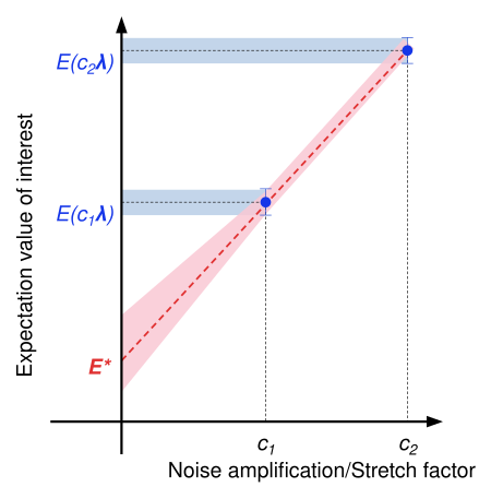
Zero-noise extrapolation (ZNE) เป็นเทคนิคลดสัญญาณรบกวนควอนตัมในการคำนวณค่าคาดหวังของ observable ทำงานโดยรัน quantum circuit ที่ระดับสัญญาณรบกวนเพิ่มขึ้น หาค่าคาดหวังที่ระดับสัญญาณรบกวนเหล่านั้น แล้ว extrapolate เพื่อประมาณค่าคาดหวังที่ไม่มีสัญญาณรบกวน ทั้งขั้นตอนการขยายสัญญาณรบกวนและการ extrapolate ทำได้หลายวิธี ในคู่มือนี้ คุณจะขยายสัญญาณรบกวนด้วย probabilistic error amplification (PEA) ตามที่เสนอใน "Evidence for the utility of quantum computing before fault tolerance" หากต้องการขยายด้วย PEA ก่อนอื่นคุณต้องสร้างโมเดลสัญญาณรบกวนที่ส่งผลต่อ entangling gate ของ circuit คุณยังขยายด้วย digital gate folding ได้ ซึ่งไม่ต้องใช้โมเดลสัญญาณรบกวนและกล่าวถึงไว้ใน คู่มือ gate folding คุณจะเรียนรู้สัญญาณรบกวนด้วย qiskit-noise-learning และ extrapolate ด้วยกลยุทธ์การ fit แบบเอกซ์โพเนนเชียลที่มีมาให้

โปรดจำไว้ว่า แม้ ZNE จะลดสัญญาณรบกวนควอนตัมได้ผลด้วยต้นทุนการสุ่มตัวอย่างต่ำกว่าวิธีอื่น แต่ก็ไม่มีขอบเขตรับประกันสำหรับ bias

ขั้นตอนการทำงานมีดังนี้:

1. ระบุ circuit และ observable
2. คำนวณค่าคาดหวังที่แน่นอนโดยใช้ตัวจำลอง statevector ของ Qiskit
3. คำนวณค่าคาดหวังที่มีสัญญาณรบกวนและยังไม่ลดสัญญาณรบกวน
4. เรียนรู้สัญญาณรบกวนของเลเยอร์ entangling ด้วย qiskit-noise-learning
5. เตรียมโปรแกรม ZNE ด้วย probabilistic error amplification และสุ่มตัวอย่าง circuit ที่ระดับสัญญาณรบกวนต่าง ๆ
6. Extrapolate ไปยังลิมิตที่ไม่มีสัญญาณรบกวน
7. เปรียบเทียบค่าคาดหวังที่ลดสัญญาณรบกวนแล้ว

ระบุ circuit และ observable

ในคู่มือนี้ คุณจะคำนวณแมกนีไทเซชันเฉลี่ยตามตำแหน่ง $\langle Z \rangle_{\text{avg}} = \frac{1}{N} \sum_{i=1}^{N} \langle Z_i \rangle$ ของแบบจำลอง Ising สนามขวาง (TFIM) แบบ Trotter บนแปด qubit ในโทโพโลยีวงแหวน คุณจะกวาดค่าความแรงของสนามขวางหลายค่าและพล็อตแมกนีไทเซชันเป็นฟังก์ชันของความแรงสนาม ในโทโพโลยีวงแหวนที่มีจำนวน qubit เป็นเลขคู่ เลเยอร์ two-qubit gate แบ่งได้เป็นสองเลเยอร์ที่ไม่ซ้ำกัน ดังที่สีแดงและสีเขียวแสดงใน coupling map ด้านล่าง การออกแบบ circuit ให้มีเลเยอร์ entangling ที่ไม่ซ้ำกันน้อยที่สุดเป็นสิ่งสำคัญหากคุณต้องการเรียนรู้โมเดลสัญญาณรบกวน เพราะเลเยอร์ที่ไม่ซ้ำกันต้องถูกเรียนรู้แยกกัน หาก circuit มีเลเยอร์ที่ไม่ซ้ำกันมากเกินไป การเรียนรู้สัญญาณรบกวนอาจทำไม่ได้เพราะต้นทุนการสุ่มตัวอย่างในการเรียนรู้หลายเลเยอร์

# Added by doQumentation — installs the packages this notebook needs if they are missing
import importlib.util

_needed = {"IPython": "IPython", "matplotlib": "matplotlib", "numpy": "numpy", "qiskit": "qiskit", "qiskit_aer": "qiskit-aer", "qiskit_ibm_runtime": "qiskit-ibm-runtime", "qiskit_mitigation": "qiskit-mitigation", "qiskit_noise_learning": "qiskit-noise-learning", "samplomatic": "samplomatic", "scipy": "scipy"}
_missing = [pip for module, pip in _needed.items()
            if importlib.util.find_spec(module) is None]
# One at a time, so a package that fails to install does not block the others
for _pip in _missing:
    %pip install -q {_pip}
if not _missing:
    print("\u2713 All required packages are installed")

import warnings

import IPython.display
import numpy as np
from qiskit.circuit import Parameter, QuantumCircuit
from qiskit.quantum_info import SparsePauliOp
from qiskit.visualization import plot_coupling_map

warnings.filterwarnings("ignore")

def trotter_circuit(num_qubits, theta, layers, num_steps):
    """Trotterized transverse-field Ising evolution: RX on every site, then a CZ layer per coupling layer."""
    circuit = QuantumCircuit(num_qubits)
    for _ in range(num_steps):
        circuit.rx(theta, range(num_qubits))
        for layer in layers:
            circuit.barrier()
            for edge in layer:
                circuit.cz(*edge)
                circuit.sdg(edge)
            circuit.barrier()
    return circuit

num_qubits = 8
trotter_steps = 15
ring_coupling = [(i, (i + 1) % num_qubits) for i in range(num_qubits)]
layers = [
    ring_coupling[0::2],
    ring_coupling[1::2],
]  # two disjoint layers of CZ gates
theta = Parameter("theta")
circuit = trotter_circuit(num_qubits, theta, layers, trotter_steps)

# Parameter values: theta in [0, 0.25 pi] - values for the transverse-field sweep
data_points = 6
parameter_values = np.linspace(0, 0.25 * np.pi, data_points).reshape(
    (data_points, 1)
)

# Define observables - Z on each site
observables = [
    SparsePauliOp("I" * (num_qubits - q - 1) + "Z" + "I" * q)
    for q in range(num_qubits)
]

print("Edges of the same color may execute their gates simultaneously.")
IPython.display.display(
    plot_coupling_map(
        num_qubits=num_qubits,
        qubit_coordinates=None,
        coupling_map=ring_coupling,
        figsize=(4, 4),
        qubit_size=150,
        line_width=5,
        line_color=[
            "red" if edge in layers[0] else "green" for edge in ring_coupling
        ],
        font_size=90,
    )
)
print("Visualization of 1 Trotter step")
trotter_circuit(num_qubits, theta, layers, 1).draw("mpl", scale=0.7)

Edges of the same color may execute their gates simultaneously.

Visualization of 1 Trotter step

คำนวณค่าคาดหวังที่แน่นอนโดยใช้ตัวจำลอง statevector ของ Qiskit

ใช้คลาส Statevector ของ Qiskit เพื่อคำนวณค่าคาดหวังที่แน่นอนของ $Z_i$ ที่แต่ละตำแหน่งสำหรับทุกค่าของ $\theta$

from qiskit.quantum_info import Statevector
import matplotlib.pyplot as plt

exact_evs = np.array(
    [
        [
            Statevector(circuit.assign_parameters([value]))
            .expectation_value(obs)
            .real
            for value in parameter_values.ravel()
        ]
        for obs in observables
    ]
)  # shape (observables, parameter values)

x_vals = parameter_values.ravel() / np.pi
fig, ax = plt.subplots(figsize=(7, 4))
ax.plot(x_vals, exact_evs.mean(axis=0), "ko-", label="Exact")
ax.set_xlabel(r"$\theta/\pi$")
ax.set_ylabel(r"$\langle Z \rangle_{\text{avg}}$")
ax.legend()
plt.tight_layout()
plt.show()

คำนวณค่าคาดหวังที่มีสัญญาณรบกวนและยังไม่ลดสัญญาณรบกวน

QuantumProgram ประกอบด้วย quantum circuit และ samplex ในรูปแบบที่เหมาะกับ Executor primitive MitigationTask.prepare สร้าง QuantumProgram จาก circuit, observable และค่าพารามิเตอร์ และใส่ box ให้ circuit ตามตัวเลือก boxing ที่กำหนด ตั้งตัวเลือก boxing measure_annotations เป็น "change_basis" ซึ่งหมุนการวัดไปยังฐานที่ต้องการ และเพิ่ม add_tags: "unique_box" เพื่อให้ตัวจำลองแมปโมเดลสัญญาณรบกวนลงบน box ของ circuit ได้ โปรแกรมจะถูก Pauli-twirl โดยค่าเริ่มต้น ซึ่งบนฮาร์ดแวร์จะเปลี่ยนสัญญาณรบกวนแบบ coherent ให้เป็นสัญญาณรบกวนแบบ Pauli ที่วิธีลดสัญญาณรบกวนสมมติไว้ num_randomizations กำหนดจำนวนอินสแตนซ์ที่ถูก twirl ของแต่ละ circuit ที่สุ่มตัวอย่าง และ shots_per_randomization กำหนดจำนวน shot ที่แต่ละอินสแตนซ์ได้รับ ผลคูณของทั้งสองจึงเป็นงบ shot ต่อ circuit

ผู้ใช้ที่เข้าถึง QPU ได้จะรันโปรแกรมด้วย Executor ที่สร้างจาก backend ของ QiskitRuntimeService ส่วนตรงนี้คุณจะส่ง AerSimulator ให้ Executor ซึ่งรันโปรแกรมในเครื่อง และใช้ตัวเลือกซิมูเลเตอร์ layer_noise_model เพื่อฉีดโมเดลสัญญาณรบกวนแบบ Pauli-Lindblad แบบสุ่มในทุกเลเยอร์ของ gate ที่สร้างพันกัน โดยสร้างด้วย random_pauli_lindblad_noise จาก qiskit-mitigation ที่มีค่าความผิดพลาดต่อ gate ในเลเยอร์ (EPLG) เท่ากับ 0.003 ซึ่งเป็นค่าทั่วไปของ QPU Heron ในปัจจุบัน

from qiskit.circuit import CircuitInstruction
from qiskit.quantum_info import PauliLindbladMap, pauli_basis
from qiskit_aer import AerSimulator
from qiskit_ibm_runtime import Executor
from qiskit_mitigation import MitigationTask, find_combined_unique_layers

def generate_random_pauli_lindblad_noise(
    layers,
    num_qubits: int,
    eplg: float = 3e-3,
    seed: int | None = None,
) -> list[tuple[CircuitInstruction, PauliLindbladMap]]:
    """Generate random Pauli-Lindblad noise over the full Pauli basis."""
    layer_noise_model = []
    for layer in layers:
        layer_instructions = layer.operation.params[0]
        contain_measurement = any(
            inst.name.startswith("measure") for inst in layer_instructions
        )
        if contain_measurement:  # do not add measurement noise
            layer_noise = PauliLindbladMap.identity(num_qubits)
        else:
            edges = [
                (inst.qubits[0]._index, inst.qubits[1]._index)
                for inst in layer_instructions
            ]  # extract the edges of the layer

            basis_paulis = [p for p in pauli_basis(2) if np.sum(p.x + p.z)]
            rng = np.random.default_rng(seed=seed)
            num_generators = len(basis_paulis)
            rates = rng.random(len(basis_paulis)) * eplg / num_generators

            layer_noise = PauliLindbladMap.from_sparse_list(
                [
                    (pauli.to_label(), edge, rate)
                    for pauli, rate in zip(basis_paulis, rates, strict=True)
                    for edge in edges
                ],
                num_qubits=num_qubits,
            )
        layer_noise_model.append((layer, layer_noise))
    return layer_noise_model

num_randomizations = 50
shots_per_randomization = 64

boxing_options = {
    "measure_annotations": "change_basis",
    "add_tags": "unique_box",
}

# find the unique layers to generate the layered noise for
box_layers = find_combined_unique_layers(
    [circuit], custom_boxing_options=boxing_options
)
layer_noise_model = generate_random_pauli_lindblad_noise(
    box_layers, num_qubits, seed=42
)

# a local noisy simulator in place of a QPU backend
noisy_executor = Executor(
    AerSimulator(),
    options={"simulator": {"layer_noise_model": layer_noise_model}},
)

task = MitigationTask()
program = task.prepare(
    circuit=circuit,
    observables=observables,
    parameters=parameter_values,
    num_randomizations=num_randomizations,
    shots_per_randomization=shots_per_randomization,
    custom_boxing_options=boxing_options,
)
program._semantic_role = "simulation"  # flag the program for the simulator
unmitigated_res = task.postprocess(noisy_executor.run(program).result())

fig, ax = plt.subplots(figsize=(7, 4))
ax.plot(x_vals, exact_evs.mean(axis=0), "k-", label="Exact")
ax.errorbar(
    x_vals,
    np.mean(unmitigated_res.data.evs, axis=0),
    np.mean(unmitigated_res.data.stds, axis=0),
    fmt="o-",
    label="Unmitigated",
)
ax.set_xlabel(r"$\theta/\pi$")
ax.set_ylabel(r"$\langle Z \rangle_{\text{avg}}$")
ax.legend()
plt.tight_layout()
plt.show()

เรียนรู้สัญญาณรบกวนของเลเยอร์ที่สร้างพันกันด้วย qiskit-noise-learning

PEA เริ่มต้นด้วยการเรียนรู้โมเดลสัญญาณรบกวนแบบ twirled ของแต่ละเลเยอร์ของ gate ที่สร้างพันกันใน circuit เราสมมติว่าเป็นโมเดลสัญญาณรบกวนแบบ Markovian ดังนั้นจึงต้องเรียนรู้เฉพาะโมเดลสัญญาณรบกวนของแต่ละเลเยอร์ที่ไม่ซ้ำกันเท่านั้น เพราะถือว่าความลึกของ circuit ไม่ส่งผลต่อช่องสัญญาณรบกวนของเลเยอร์ที่สร้างพันกันเลเยอร์นั้น ยิ่งโมเดลสัญญาณรบกวนที่เรียนรู้ได้แม่นยำเท่าไร การขยายสัญญาณรบกวนก็ยิ่งแม่นยำเท่านั้น

เราใช้ qiskit-noise-learning เพื่อเรียนรู้สัญญาณรบกวน ตัวเรียนรู้จะทำซ้ำแต่ละเลเยอร์ fragment_depths ครั้งใน circuit สำหรับเรียนรู้ ทำ twirl แต่ละ circuit num_randomizations ครั้ง และฟิตการสลายตัวของค่า fidelity ที่วัดได้เข้ากับโมเดล Pauli-Lindblad โค้ดต่อไปนี้วาดโมเดลสัญญาณรบกวนที่เรียนรู้ได้ โดยรวมสองเลเยอร์ไว้ในแผนที่เดียว แต่ละ qubit เป็นแผนภูมิวงกลมของอัตรา X, Y และ Z น้ำหนัก 1 ที่รวมจากสองเลเยอร์ และแต่ละเส้นเชื่อมแสดงอัตราน้ำหนัก 2 ที่เรียนรู้ได้ อัตรา 3e-4 หมายความว่าความผิดพลาดนั้นเกิดขึ้นประมาณสามครั้งในทุก 10,000 ครั้งที่ใช้เลเยอร์

from qiskit.providers.fake_provider import GenericBackendV2
from qiskit.quantum_info import PauliList
from qiskit_ibm_runtime.results import LayerError, PauliLindbladError
from qiskit_ibm_runtime.visualization.embeddings import Embedding
from qiskit_mitigation import PEA
from qiskit_noise_learning.aer_executor import AerExecutor
from qiskit_noise_learning.noise_learner import LearningOptions, NoiseLearner
from samplomatic import InjectNoise, Tag
from samplomatic.utils import get_annotation

backend = GenericBackendV2(
    num_qubits=num_qubits,
    basis_gates=["id", "rz", "sx", "x", "cz"],
    coupling_map=ring_coupling,
)

task_pea = PEA()
# learn only the layers PEA will inject noise into, i.e. not the measurement layer
pea_layers = [
    layer
    for layer in task_pea.find_unique_layers(circuit, boxing_options)
    if get_annotation(layer.operation, InjectNoise)
]

learning_options = LearningOptions(
    fragment_depths=[2, 4, 8, 16],
    num_randomizations=50,
    shots_per_randomizations=64,
)
# qiskit-noise-learning is not compatible with the Executor in local mode,
# and requires the simulator present in the package for running simulation
noise_dict = {
    get_annotation(layer.operation, Tag).ref: noise_layer
    for layer, noise_layer in layer_noise_model
}
noise_learner_simulator = AerExecutor(
    qasm_simulator=AerSimulator(), noise_dict=noise_dict
)
learner = NoiseLearner(
    backend, options=learning_options, executor=noise_learner_simulator
)
learned_noise = (
    learner.run(pea_layers).result().to_dict()
)  # keyed by InjectNoise reference

# Draw the learned model on the ring, laid out as a square with the qubits in ring order.
# Composing the two layers' maps sums their rates, giving one map over all the ring's edges.
embedding = Embedding(
    [(0, 0), (0, 2), (0, 4), (2, 4), (4, 4), (4, 2), (4, 0), (2, 0)],
    ring_coupling,
)
first, second = learned_noise.values()
learned_model = first.compose(second).simplify()
error = PauliLindbladError(
    PauliList(
        learned_model.get_qubit_sparse_pauli_list_copy().to_pauli_list()
    ),
    learned_model.rates,
)
fig = LayerError(circuit, list(range(num_qubits)), error).draw_map(
    embedding, radius=0.4, height=460, width=620
)
fig.update_traces(
    marker={
        "cmin": 0,
        "cmax": max(learned_model.rates),
        "colorbar": {"tickformat": ".1e", "title": "rate"},
    },
    selector={"mode": "markers"},
)
fig.show()

เตรียมโปรแกรม ZNE ที่ใช้การขยายความผิดพลาดแบบความน่าจะเป็น และสุ่มตัวอย่าง circuit ที่มีสเกลสัญญาณรบกวนต่างกัน

ตรงนี้คุณจะเตรียมโปรแกรม ZNE ที่มี circuit ซึ่งสเกลสัญญาณรบกวนเพิ่มขึ้นเรื่อยๆ ใน PEA แต่ละ noise factor แทนจำนวนเท่าของสัญญาณรบกวนที่เรียนรู้ได้ซึ่ง circuit ต้องเจอ: noise factor 2.0 จะฉีดช่องสัญญาณรบกวนที่เรียนรู้ได้ของแต่ละเลเยอร์เพิ่มอีกหนึ่งชุดหลังเลเยอร์นั้น ซ้อนทับกับสัญญาณรบกวนที่เลเยอร์นั้นมีอยู่แล้ว เนื่องจาก PEA ปรับสเกลอัตราสัญญาณรบกวนที่เรียนรู้ได้โดยตรงแทนการทำ gate ซ้ำ จึงใช้ noise factor ค่าใดก็ได้ รวมถึงค่าที่ไม่ใช่จำนวนเต็ม และตัว circuit เองไม่ถูกแก้ไข: รายการในโปรแกรมใช้ circuit แม่แบบเดียวกัน และต่างกันแค่สัญญาณรบกวนที่ samplex ฉีดเข้าไป สัญญาณรบกวนที่ฉีดจะถูกสุ่มหนึ่งครั้งต่อหนึ่ง randomization ดังนั้นความคลาดเคลื่อนทางสถิติของ PEA จึงถูกควบคุมด้วยจำนวน randomization ไม่ใช่จำนวน shot ต่อ randomization เราจึงใช้ randomization จำนวนมากโดยให้แต่ละอันมีไม่กี่ shot และคงจำนวน shot ทั้งหมดให้เท่ากับโปรแกรมที่ไม่ได้ลดสัญญาณรบกวน สิ่งสำคัญคืออย่าใช้ randomization น้อยเกินไป ไม่เช่นนั้นอาจเจออคติจากการสุ่มตัวอย่างในการฉีดสัญญาณรบกวน

โอเวอร์เฮดการสุ่มตัวอย่างทั้งหมดเพิ่มขึ้นเป็นเส้นตรงตามจำนวน noise factor

noise_factors = [1, 2, 3]
program_pea = task_pea.prepare(
    circuit=circuit,
    observables=observables,
    parameters=parameter_values,
    num_randomizations=200,
    shots_per_randomization=16,
    custom_boxing_options=boxing_options,
    noise_maps=learned_noise,
    noise_factors=noise_factors,
)

สุดท้าย รันโปรแกรมบนซิมูเลเตอร์ที่มีสัญญาณรบกวน ผลลัพธ์จะถูกนำไปใช้ในการ extrapolate ในขั้นตอนถัดไป

program_pea._semantic_role = (
    "simulation"  # flag the program for the simulator
)
job_pea_results = noisy_executor.run(program_pea).result()

Extrapolate ไปยังขีดจำกัดที่ไม่มีสัญญาณรบกวน

เมื่อคุณมีข้อมูลของแต่ละสเกลสัญญาณรบกวนแล้ว คุณสามารถฟิตฟังก์ชันเข้ากับข้อมูล แล้ว extrapolate กลับไปยังค่าที่ไม่มีสัญญาณรบกวนเพื่อประมาณค่าคาดหมายของ observable ที่ปราศจากสัญญาณรบกวน ภายใต้สัญญาณรบกวนแบบ Pauli observable จะสลายตัวแบบเอกซ์โพเนนเชียลตาม noise factor ดังนั้นคุณจะเลือก extrapolator แบบเอกซ์โพเนนเชียลเป็นตัวเลือกแรก และถอยไปใช้แบบเชิงเส้นหากการฟิตแบบเอกซ์โพเนนเชียลล้มเหลว เพื่อให้เห็นภาพการ extrapolate ให้พล็อตค่า magnetization เฉลี่ยตามตำแหน่งที่คำนวณได้ที่แต่ละ noise factor, เส้นฟิตแบบเอกซ์โพเนนเชียล และค่าเฉลี่ยตามตำแหน่งของค่าคาดหมายที่ extrapolate ได้ที่จุดไร้สัญญาณรบกวน เราเห็นว่าการฟิตต่ำกว่าค่าจริงเล็กน้อยสำหรับ observable นี้

from scipy.optimize import curve_fit

pea_mitigated_res = task_pea.postprocess(
    job_pea_results, extrapolator=["exponential", "linear"]
)

# The result holds the expectation value at each noise factor and the extrapolated value for
# every observable; we average them over the sites and fit the same model to draw the curve.
angle = 3  # theta = 0.15 pi, the angle with the largest unmitigated error
amplifications = pea_mitigated_res.data.evs_noise_factors[:, angle, :].mean(
    axis=0
)
x_fit = np.linspace(0, max(noise_factors), 51)
params, _ = curve_fit(
    lambda x, a, b: a * np.exp(b * x),
    noise_factors,
    amplifications,
    p0=[1.0, -0.1],
)

plt.plot(
    noise_factors, amplifications, "o", color="red", label="amplifications"
)
plt.plot(
    x_fit,
    params[0] * np.exp(params[1] * x_fit),
    "--",
    color="black",
    label="exponential fit",
)
plt.plot(
    [0],
    pea_mitigated_res.data.evs[:, angle].mean(),
    "*",
    color="black",
    markersize=15,
    label="extrapolation",
)
plt.plot(
    [0],
    exact_evs[:, angle].mean(),
    "_",
    color="red",
    markersize=15,
    markeredgewidth=3,
    label="exact",
)
plt.xlabel("noise factor")
plt.ylabel(r"$\langle Z \rangle_{\text{avg}}$")
plt.legend()
plt.show()

เปรียบเทียบค่าคาดหมายที่ลดสัญญาณรบกวนแล้ว

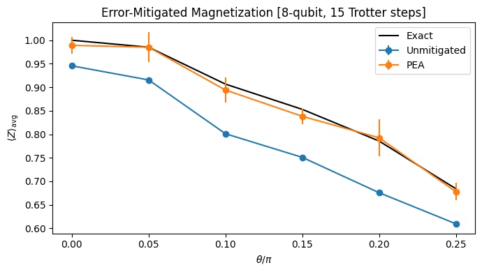
พล็อตค่า magnetization เฉลี่ยตามตำแหน่งของแต่ละวิธีตลอดช่วงมุมการหมุนของ Ising PEA กู้ค่า magnetization ที่แน่นอนได้ภายในแถบความคลาดเคลื่อน ขณะที่ผลลัพธ์ที่ไม่ได้ลดสัญญาณรบกวนมีอคติต่ำกว่าค่านั้นมาก

results = {
    "Unmitigated": unmitigated_res,
    "PEA": pea_mitigated_res,
}

fig, ax = plt.subplots(figsize=(7, 4))
ax.plot(x_vals, exact_evs.mean(axis=0), "k-", label="Exact")
for label, res in results.items():
    ax.errorbar(
        x_vals,
        np.mean(res.data.evs, axis=0),
        np.mean(res.data.stds, axis=0),
        fmt="o-",
        label=label,
    )
ax.set_xlabel(r"$\theta/\pi$")
ax.set_ylabel(r"$\langle Z \rangle_{\text{avg}}$")
ax.legend()
ax.set_title(
    f"Error-Mitigated Magnetization [{num_qubits}-qubit, {trotter_steps} Trotter steps]"
)
plt.tight_layout()
plt.show()