การหักล้างข้อผิดพลาดเชิงความน่าจะเป็นด้วยโมเดลสัญญาณรบกวนเชิงตรรกะ

ประมาณการเวลาใช้งาน: 28 นาที บนโปรเซสเซอร์ Heron r3 (หมายเหตุ: นี่เป็นเพียงการประมาณการเท่านั้น เวลาที่ใช้จริงอาจแตกต่างกันไป)

In this tutorial we will evaluate observables of a 22-site Ising model on a hexagonal lattice using a Heron QPU, which has a heavy-hexagonal qubit topology. Many demonstrations on Heron QPUs focus on systems defined on heavy-hexagonal lattices to match the system's connectivity; however, hexagonal models tend to be more interesting to study as they appear more commonly in nature and are more difficult to simulate classically due to their denser connectivity. Since the qubit topology of the QPU cannot directly support the connectivity of a hexagonal lattice, we must decide how to efficiently embed the hexagonal model onto the qubit topology. In this example we represent each site in the Ising model with a qubit lying on a vertex of the heavy-hex QPU lattice. We use the qubits on the edges (mediator qubits) to facilitate entanglement between the Ising qubits on the vertices. Additionally, the mediator qubits implement entanglement in such a way that they are always expected to return to the ground state $|0\rangle$. If a mediator qubit measures $|1\rangle$, it indicates that a logical error occurred during circuit execution; postselecting only samples with no detected errors on the mediator qubits yields a smaller distribution of logical samples that might have a higher fidelity than the raw, noisy distribution. Not only can we detect that an error occurred by measuring a mediator qubit, we can also determine exactly which logical errors that qubit is capable of detecting throughout the circuit. Removing the noise generators the mediator qubits' symmetry checks are capable of detecting from a noise model leaves a reduced noise model, which can be mitigated using techniques such as probabilistic error cancellation (PEC).

ในตัวอย่าง notebook นี้ เราจะผสานเทคนิคการตรวจจับข้อผิดพลาดที่อธิบายไว้ข้างต้นเข้ากับ PEC เพื่อต่อต้านสัญญาณรบกวนควอนตัมได้อย่างมีประสิทธิภาพมากกว่าการใช้เทคนิคใดเทคนิคหนึ่งเพียงอย่างเดียว เราจะใช้ 49 qubit เพื่อฝังโมเดล Ising ขนาด 22 qubit และใช้ mediator qubit เพิ่มอีก 27 ตัวสำหรับการตรวจจับข้อผิดพลาด เราจะรัน PEC บนช่องสัญญาณรบกวนที่ผ่านการ postselect แล้วเพื่อลดสัญญาณรบกวนที่หลบเลี่ยงการตรวจสอบสมมาตร นอกเหนือจากการผสานการตรวจจับข้อผิดพลาดกับ PEC แล้ว เราจะใช้เทคนิคต่าง ๆ เช่น การลดข้อผิดพลาดการอ่านค่าแบบ TREX และการตรวจสอบข้อผิดพลาดแบบ non-Markovian เพื่อต่อสู้กับผลของสัญญาณรบกวนควอนตัมเพิ่มเติม

ขั้นตอนการทำงานมีดังนี้:

1. จำลองค่าคาดหวังของ observable แบบคลาสสิกสำหรับโมเดล hex-Ising ขนาด 22 qubit
2. สร้างโมเดล hex-Ising ที่ตรวจจับข้อผิดพลาดขนาด 49 qubit ด้วยวงจรควอนตัมและ transpile ไปยัง backend ของ QPU
3. ระบุเลเยอร์การพัวพันในวงจรด้วย samplomatic เราจะเรียนรู้และลดสัญญาณรบกวนที่ส่งผลต่อเลเยอร์การพัวพันเหล่านี้
4. เพิ่มการตรวจสอบข้อผิดพลาดแบบ non-Markovian ให้กับวงจร
5. เรียนรู้สัญญาณรบกวนของ gate และการอ่านค่าที่ส่งผลต่อวงจร
6. ตัดพจน์ที่ตรวจพบโดยการตรวจสอบสมมาตรออกจากโมเดลสัญญาณรบกวน
7. สุ่มตัวอย่างวงจรที่ตรวจจับข้อผิดพลาด โดย postselect เฉพาะตัวอย่างที่ผ่านการตรวจสอบสมมาตรและ non-Markovian ทั้งหมด และใช้การลดข้อผิดพลาดการอ่านค่าแบบ TREX สำหรับการคำนวณค่าคาดหวังทั้งหมด
   • สุ่มตัวอย่างวงจรที่ตรวจจับข้อผิดพลาด
   • สุ่มตัวอย่างวงจรที่ตรวจจับข้อผิดพลาดด้วย PEC แต่ไม่ postselect ตามการตรวจสอบสมมาตร และลดสัญญาณรบกวนทั้งหมดที่เรียนรู้มา
   • สุ่มตัวอย่างวงจรที่ตรวจจับข้อผิดพลาดด้วย PEC โดย postselect ตามการตรวจสอบสมมาตร และลดเฉพาะสัญญาณรบกวนที่ไม่สามารถตรวจพบได้ด้วยการตรวจสอบเท่านั้น
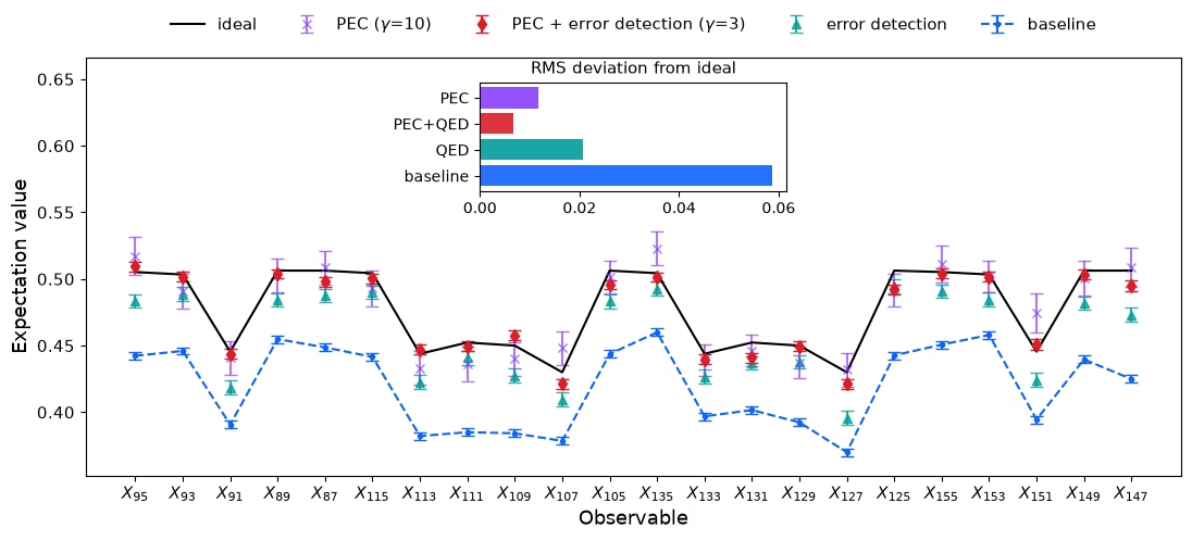
8. คำนวณค่าคาดหวังและเปรียบเทียบกลยุทธ์ต่าง ๆ สังเกตว่า QED+PEC สามารถหักล้างสัญญาณรบกวนที่ส่งผลต่อการทดลองได้อย่างมีประสิทธิภาพมากกว่าการใช้วิธีใดวิธีหนึ่งเพียงอย่างเดียว และให้ค่าคาดหวังที่ลู่เข้าโดยใช้จำนวนช็อตน้อยกว่าที่ PEC เพียงอย่างเดียวต้องการมาก

ข้อกำหนดเบื้องต้น

ก่อนเริ่มบทเรียนนี้ ให้รันคำสั่งต่อไปนี้เพื่อติดตั้งแพ็กเกจที่จำเป็นทั้งหมด:

%pip install networkx numpy "qiskit[visualization]" "qiskit-ibm-runtime[visualization]" samplomatic qiskit-mitigation matplotlib "qiskit-noise-learning @ git+https://github.com/Qiskit/qiskit-noise-learning.git@ieee-demo-2026" เซลล์ที่ยุบไว้ด้านล่างกำหนด figure helper ที่ใช้ตลอดทั้ง notebook นี้

คลิกเพื่อดู figure helper

# Added by doQumentation — installs the packages this notebook needs if they are missing
import importlib.util

_needed = {"matplotlib": "matplotlib", "networkx": "networkx", "numpy": "numpy", "qiskit": "qiskit", "qiskit_ibm_runtime": "qiskit-ibm-runtime", "qiskit_mitigation": "qiskit-mitigation", "qiskit_noise_learning": "qiskit-noise-learning@git+https://github.com/Qiskit/qiskit-noise-learning.git@ieee-demo-2026", "samplomatic": "samplomatic"}
_missing = [pip for module, pip in _needed.items()
            if importlib.util.find_spec(module) is None]
# One at a time, so a package that fails to install does not block the others
for _pip in _missing:
    %pip install -q {_pip}
if not _missing:
    print("\u2713 All required packages are installed")

# Figure helpers for this notebook (collapsed): all plotting and styling lives here.
# The chip maps follow the style of Fig. 30 of arXiv:2607.25998.

from math import comb

import matplotlib.pyplot as plt
from matplotlib import cm
from matplotlib.colors import BoundaryNorm
from matplotlib.patches import Circle, Rectangle, Wedge

# one typography scheme for every figure in the notebook
plt.rcParams.update(
    {
        "font.size": 13,
        "axes.titlesize": 15,
        "axes.labelsize": 13,
        "xtick.labelsize": 11,
        "ytick.labelsize": 11,
        "legend.fontsize": 11,
    }
)

def x_labels(layout, n_data):
    """Per-observable tick labels carrying the physical qubit indices (site i = qubit i)."""
    return [f"$X_{{{layout[i]}}}$" for i in range(n_data)]

def plot_layout(backend, layout, n_data):
    """Chip cartoon of the embedding: data qubits green, check qubits orange."""
    from qiskit.visualization import plot_coupling_map

    return plot_coupling_map(
        num_qubits=backend.num_qubits,
        qubit_coordinates=None,
        coupling_map=list(backend.coupling_map.get_edges()),
        figsize=(9, 9),
        qubit_color=[
            "#4CAF50"
            if q in layout[:n_data]
            else "#FF9800"
            if q in layout[n_data:]
            else "#DDDDDD"
            for q in range(backend.num_qubits)
        ],
        qubit_size=220,
        line_width=2,
        font_size=90,
    )

def plot_exact(obs_exact, tick_labels, title):
    plt.figure(figsize=(12, 4))
    plt.plot(obs_exact, "o-")
    plt.title(title)
    plt.xticks(np.arange(len(obs_exact)), tick_labels)
    plt.xlabel("Observable")
    plt.ylabel(r"$\langle X \rangle$")
    plt.grid()

def draw_toy_circuit(
    generate_ed_ising, zz_coeff, x_coeff, include_checks=True
):
    """The boxing pipeline on a 3-plaquette-ring miniature (1 Trotter step) so the box
    structure is legible; every box carries the Twirl / InjectNoise annotations, and with
    ``include_checks`` the terminal xslow non-Markovian error check pattern is appended as in the
    production pipeline."""
    import networkx as nx
    from qiskit.circuit import ClassicalRegister
    from qiskit_mitigation.postselection import XSlowGate
    from samplomatic.transpiler import generate_boxing_pass_manager

    toy, _, _ = generate_ed_ising(nx.cycle_graph(3), 1, zz_coeff, x_coeff)
    toy.add_register(
        ClassicalRegister(3, "data"), ClassicalRegister(3, "check")
    )
    toy.barrier()
    toy.measure(range(3), range(3))
    toy.measure(range(3, 6), range(3, 6))
    toy_boxed = generate_boxing_pass_manager(
        enable_gates=True,
        enable_measures=True,
        inject_noise_targets="gates",
        inject_noise_strategy="individual_modification",
        inject_noise_site="after",
        twirling_strategy="active_circuit",
        measure_annotations="all",
    ).run(toy)
    if include_checks:
        toy_boxed.add_register(
            ClassicalRegister(3, "data_ps"), ClassicalRegister(3, "check_ps")
        )
        toy_boxed.barrier()
        for qb in range(6):
            toy_boxed.append(XSlowGate(), [qb])
        toy_boxed.measure(range(3), toy_boxed.cregs[2])
        toy_boxed.measure(range(3, 6), toy_boxed.cregs[3])
    return toy_boxed.draw("mpl", fold=-1, scale=0.6)

# --- chip-level noise maps ---------------------------------------------------------

BANDS = [1e-5, 2e-5, 3e-5, 4e-5, 6e-5, 1e-4, 2e-4, 3e-4, 4e-4, 6e-4, 1e-3]
CMAP = plt.get_cmap("YlOrBr")
NORM = BoundaryNorm(BANDS, CMAP.N, extend="both")

def _color(rate):
    return (
        "white"
        if rate < BANDS[0]
        else CMAP(NORM(min(rate, BANDS[-1] * 0.999)))
    )

def _layer_sparse(mit, weights):
    """Per-layer labelled terms from the saved run, box-local -> physical qubits."""
    phys = np.sort(mit["layout"])
    return [
        [
            (p, tuple(int(phys[q]) for q in qs if q >= 0), r)
            for p, qs, r in zip(
                mit[f"label_paulis_{i}"],
                mit[f"label_qubits_{i}"],
                w,
                strict=True,
            )
        ]
        for i, w in enumerate(weights)
    ]

def _aggregate(layers):
    """w1[qubit][P] and w2[(a,b)][PaPb]: rates summed over the 3 layers."""
    w1, w2 = {}, {}
    for terms in layers:
        for p, qs, r in terms:
            if len(qs) == 1:
                w1.setdefault(qs[0], dict.fromkeys("XYZ", 0.0))[p] += r
            else:
                (a, pa), (b, pb) = sorted(zip(qs, p, strict=True))
                w2.setdefault(
                    (a, b), {x + y: 0.0 for x in "XYZ" for y in "XYZ"}
                )[pa + pb] += r
    return w1, w2

def draw_noise_map(mit, backend, reduced=False):
    """Chip map of the learned model: X/Y/Z wheel per qubit, 3x3 two-qubit Pauli grid per
    coupler, log-banded colors, dashed outlines for unused hardware.

    With ``reduced=True``, keeps only the error terms the checks cannot see: detectability
    depends on circuit position, so each layer's 0/1 site scales are averaged over its uses.
    """
    from qiskit_ibm_runtime.visualization.embeddings import Embedding

    if reduced:
        scales = [
            mit["site_scales"][mit["site_layer"] == i].mean(axis=0)
            for i in range(3)
        ]
        weights = [mit[f"rates_{i}"] * scales[i] for i in range(3)]
        title = f"Reduced noise model ($\\gamma$ = {mit['gammas'][1]:.1f})"
    else:
        weights = [mit[f"rates_{i}"] for i in range(3)]
        title = f"Full noise model ($\\gamma$ = {mit['gammas'][0]:.0f})"
    w1, w2 = _aggregate(_layer_sparse(mit, weights))

    xy = np.array(
        [(c, -r) for r, c in Embedding.from_backend(backend).coordinates]
    )
    fig, ax = plt.subplots(figsize=(13, 7))
    for a, b in {tuple(sorted(e)) for e in backend.coupling_map.get_edges()}:
        if (
            (
                a,
                b,
            )
            in w2
        ):  # 3x3 Pauli grid laid along the bond (columns: qubit a, rows: qubit b)
            d = xy[b] - xy[a]
            u = d / np.hypot(*d)
            v = np.array([-u[1], u[0]])
            cl, cw = (np.hypot(*d) - 0.6) / 3, 0.17
            for i, Pa in enumerate("XYZ"):
                for j, Pb in enumerate("XYZ"):
                    ax.add_patch(
                        Rectangle(
                            xy[a] + u * (0.3 + i * cl) + v * ((j - 1.5) * cw),
                            cl,
                            cw,
                            angle=np.degrees(np.arctan2(u[1], u[0])),
                            facecolor=_color(w2[a, b][Pa + Pb]),
                            edgecolor="black",
                            lw=0.4,
                            zorder=2,
                        )
                    )
        else:
            ax.plot(
                *zip(xy[a], xy[b], strict=True),
                ls="--",
                lw=0.7,
                color="black",
                alpha=0.5,
                zorder=1,
            )
    for q, (xq, yq) in enumerate(xy):
        if q in w1:  # three-sector wheel: X top, Y lower left, Z lower right
            for P, t0 in (("X", 30), ("Y", 150), ("Z", 270)):
                ax.add_patch(
                    Wedge(
                        (xq, yq),
                        0.3,
                        t0,
                        t0 + 120,
                        facecolor=_color(w1[q][P]),
                        edgecolor="black",
                        lw=0.6,
                        zorder=3,
                    )
                )
            ax.annotate(
                str(q),
                (xq + 0.39, yq - 0.39),
                fontsize=9,
                color="gray",
                ha="left",
                va="top",
                zorder=4,
            )  # southeast, clear of the bond grids
        else:
            ax.add_patch(
                Circle(
                    (xq, yq),
                    0.24,
                    facecolor="none",
                    edgecolor="black",
                    ls="--",
                    lw=0.7,
                    alpha=0.5,
                    zorder=3,
                )
            )
    ux = xy[sorted(w1)]
    ax.set_xlim(ux[:, 0].min() - 2.2, ux[:, 0].max() + 2.2)
    ax.set_ylim(ux[:, 1].min() - 1.6, ux[:, 1].max() + 1.6)
    ax.set_aspect("equal")
    ax.axis("off")
    ax.set_title(title, fontsize=15)
    cb = fig.colorbar(
        cm.ScalarMappable(norm=NORM, cmap=CMAP),
        ax=ax,
        fraction=0.035,
        pad=0.02,
        extend="both",
        ticks=BANDS,
    )
    cb.set_label("coefficient (log bands; white < 1e-05)", fontsize=11)
    cb.ax.set_yticklabels(
        [f"{b:.0e}".replace("e-0", "e-") for b in BANDS], fontsize=10
    )
    _noise_map_legends(fig, ax)

def _noise_map_legends(fig, ax):
    """Weight-1 wheel and weight-2 grid keys, in a reserved band left of the lattice."""
    fig.subplots_adjust(left=0.17)
    axl = ax.inset_axes([-0.185, 0.70, 0.13, 0.24])
    for P, t0 in (("X", 30), ("Y", 150), ("Z", 270)):
        axl.add_patch(
            Wedge(
                (0.5, 0.45),
                0.38,
                t0,
                t0 + 120,
                facecolor="white",
                edgecolor="black",
                lw=0.8,
            )
        )
        axl.annotate(
            P,
            (
                0.5 + 0.2 * np.cos(np.radians(t0 + 60)),
                0.45 + 0.2 * np.sin(np.radians(t0 + 60)),
            ),
            ha="center",
            va="center",
            fontsize=9,
        )
    axl.set_title("weight-1", fontsize=10)
    axl.set_xlim(0, 1)
    axl.set_ylim(0, 1)
    axl.set_aspect("equal")
    axl.axis("off")
    axm = ax.inset_axes([-0.185, 0.32, 0.14, 0.30])
    for i, Pa in enumerate("XYZ"):
        for j, Pb in enumerate("XYZ"):
            axm.add_patch(
                Rectangle(
                    (i / 3, 1 - (j + 1) / 3),
                    1 / 3,
                    1 / 3,
                    facecolor="white",
                    edgecolor="black",
                    lw=0.6,
                )
            )
            axm.annotate(
                Pa + Pb,
                ((i + 0.5) / 3, 1 - (j + 0.5) / 3),
                ha="center",
                va="center",
                fontsize=7.5,
            )
        axm.annotate(Pa, ((i + 0.5) / 3, 1.08), ha="center", fontsize=8.5)
        axm.annotate(
            "XYZ"[i],
            (-0.13, 1 - (i + 0.5) / 3),
            ha="center",
            va="center",
            fontsize=8.5,
        )
    axm.annotate("qubit a", (0.5, 1.27), ha="center", fontsize=9)
    axm.annotate(
        "qubit b", (-0.33, 0.5), rotation=90, va="center", fontsize=9
    )
    axm.set_xlim(-0.35, 1.05)
    axm.set_ylim(-0.05, 1.35)
    axm.set_aspect("equal")
    axm.axis("off")

# --- run diagnostics ---------------------------------------------------------------

def plot_trex(trex_rescale, tick_labels):
    _fig, axt = plt.subplots(figsize=(12, 3))
    axt.stem(np.arange(len(trex_rescale)), (trex_rescale - 1) * 100)
    axt.set_xticks(np.arange(len(trex_rescale)), tick_labels)
    axt.set_xlabel("Observable")
    axt.set_ylabel("Readout correction (%)")
    axt.set_title("TREX rescale factors")
    plt.tight_layout()

def plot_postselection(mit):
    """Accepted shots per PEC randomization against a single binomial at the mean
    acceptance rate: agreement means acceptance is independent of the sampled circuit
    instance, the condition under which pooling accepted shots across randomizations
    is a consistent estimator."""
    _fig, ax = plt.subplots(figsize=(7.5, 3.8))
    counts = mit["acc_counts_post"]
    K, p = 64, counts.mean() / 64
    ks = np.arange(K + 1)
    pmf = np.array([comb(K, k) * p**k * (1 - p) ** (K - k) for k in ks])
    ax.hist(
        counts,
        bins=np.arange(-0.5, K + 1.5),
        density=True,
        alpha=0.6,
        color="#da1e28",
        label="measured",
    )
    ax.plot(ks, pmf, "k-", lw=1.5, label=f"Binomial(64, {p:.3f})")
    ax.set_xlim(-0.5, max(int(counts.max()) + 3, 20))
    ax.set_xlabel("Accepted shots per randomization")
    ax.set_ylabel("Probability")
    ax.legend()
    ax.grid(alpha=0.4)
    plt.tight_layout()

def plot_convergence(mit, obs_exact, n_data):
    """Running site-averaged estimate vs. randomizations for both PEC arms (the S5-consistent
    signed-ratio estimator, evaluated on growing prefixes of the sweep)."""

    def running(prefix):
        bits = np.squeeze(
            np.unpackbits(mit[f"data_{prefix}"], axis=-1)[..., :n_data]
            ^ mit[f"flips_{prefix}"]
        )
        mask = np.squeeze(mit[f"mask_{prefix}"])
        signs = 1 - 2 * (np.squeeze(mit[f"signs_{prefix}"]).sum(axis=-1) % 2)
        qv = (1 - 2 * bits.astype(int)) * mit["trex_rescale"]
        u = (
            (signs[:, None, None] * mask[..., None] * qv)
            .sum(axis=1)
            .mean(axis=1)
        )
        v = signs * mask.sum(axis=1)
        Rs = np.arange(500, len(u) + 1, 500)
        est, err = [], []
        for R in Rs:
            e = u[:R].sum() / v[:R].sum()
            est.append(e)
            err.append(
                np.sqrt(((u[:R] - e * v[:R]) ** 2).sum()) / abs(v[:R].sum())
            )
        return Rs, np.array(est), np.array(err)

    _fig, ax = plt.subplots(figsize=(12, 5))
    ideal_avg = float(np.mean(obs_exact))
    ax.axhline(ideal_avg, color="black", label="ideal")
    ax.fill_between(
        [-400, 24000],
        ideal_avg - 0.025,
        ideal_avg + 0.025,
        color="grey",
        alpha=0.22,
        label=r"$\pm 0.025$",
    )
    for prefix, label, color in (
        ("van", "vanilla PEC", "#8a3ffc"),
        ("post", "PEC + error detection", "#da1e28"),
    ):
        Rs, est, err = running(prefix)
        ax.errorbar(
            Rs,
            est,
            yerr=err,
            marker="o",
            linestyle="",
            markerfacecolor="none",
            color=color,
            alpha=0.85,
            capsize=3,
            label=label,
        )
    ax.set_xlim(-400, 24000)
    ax.set_ylim(ideal_avg - 0.08, ideal_avg + 0.08)
    ax.set_xlabel("# randomizations")
    ax.set_ylabel(r"Site-averaged $\langle X \rangle$")
    ax.legend(ncols=2)

def plot_final(
    obs_exact, baseline, ed, pec, post, gammas, tick_labels, title
):
    """Per-site <X> for every method, with an rms-deviation inset.
    baseline/ed/pec/post are (values, errors) pairs; gammas is (gamma, gamma_post)."""
    x = np.arange(len(obs_exact))
    _fig, ax = plt.subplots(figsize=(13, 5))
    h_ideal = ax.errorbar(
        x, obs_exact, fmt="-", capsize=4, label="ideal", color="black"
    )
    h_base = ax.errorbar(
        x,
        baseline[0],
        yerr=baseline[1],
        fmt=".--",
        capsize=4,
        label="baseline",
        color="#0f62fe",
    )
    h_ed = ax.errorbar(
        x,
        ed[0],
        yerr=ed[1],
        fmt="^",
        capsize=4,
        label="error detection",
        color="#009d9a",
        alpha=0.8,
    )
    h_pec = ax.errorbar(
        x,
        pec[0],
        yerr=pec[1],
        fmt="x",
        capsize=4,
        label=f"PEC ($\\gamma$={gammas[0]:.0f})",
        color="#8a3ffc",
        alpha=0.7,
    )
    h_post = ax.errorbar(
        x,
        post[0],
        yerr=post[1],
        fmt="d",
        capsize=4,
        label=f"PEC + error detection ($\\gamma$={gammas[1]:.0f})",
        color="#da1e28",
    )
    ax.set_xticks(x, tick_labels)
    ax.set_xlabel("Observable")
    ax.set_ylabel("Expectation value")
    # Set the y-axis range using the ideal, baseline, error detection, and PEC + error
    # detection curves, including error bars. Exclude PEC-only values when setting the
    # range so large fluctuations do not make the other curves difficult to distinguish.
    # PEC-only values may fall outside the visible range. Leave room above for the inset.
    series = [np.asarray(obs_exact)] + [
        np.asarray(v) + s * np.asarray(e)
        for v, e in (baseline, ed, post)
        for s in (-1, 1)
    ]
    lo, hi = min(a.min() for a in series), max(a.max() for a in series)
    span = max(hi - lo, 0.1)
    ax.set_ylim(lo - 0.1 * span, hi + 1.05 * span)
    # legend ordered to match the curves' vertical positions in the chart
    ax.legend(
        handles=[h_ideal, h_pec, h_post, h_ed, h_base],
        ncols=5,
        loc="lower center",
        bbox_to_anchor=(0.5, 1.02),
        frameon=False,
    )
    ax.set_title(title, pad=44)

    # inset: rows bottom-to-top so it reads top-to-bottom: PEC, PEC+ED, ED, baseline
    axi = ax.inset_axes([0.36, 0.68, 0.28, 0.26])
    methods = [
        ("baseline", baseline[0], "#0f62fe"),
        ("QED", ed[0], "#009d9a"),
        ("PEC+QED", post[0], "#da1e28"),
        ("PEC", pec[0], "#8a3ffc"),
    ]
    for k, (_nm, vals, color) in enumerate(methods):
        axi.barh(
            k,
            np.sqrt(np.mean((vals - np.array(obs_exact)) ** 2)),
            color=color,
            alpha=0.9,
        )
    axi.set_yticks(range(4), [m[0] for m in methods], fontsize=10)
    axi.set_title("RMS deviation from ideal", fontsize=11)
    axi.tick_params(labelsize=10)
    axi.patch.set_alpha(1.0)
    axi.set_zorder(5)

จำลอง $\langle X \rangle_i$ แบบคลาสสิกสำหรับแต่ละไซต์ในโมเดล hex-Ising ขนาด 22 qubit

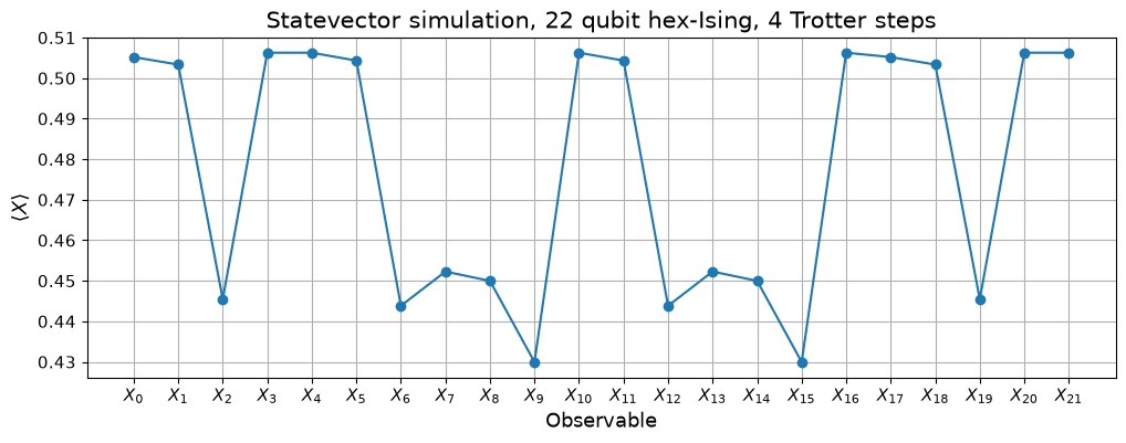
ก่อนอื่น เราใช้คลาส Statevector ของ Qiskit เพื่อจำลองค่าเป้าหมายที่แน่นอนสำหรับการทดลองของเรา แม้ว่าปัญหาขนาด 22 qubit ที่เรากำลังแก้จะสามารถคำนวณได้แบบคลาสสิก แต่ตัวจำลอง statevector ของ Qiskit จะไม่สามารถขยายไปสู่การสาธิตที่ใหญ่กว่านี้มากได้ และหากต้องการขยายไปเกิน 50 qubit หรือประมาณนั้น เราจะต้องใช้เทคนิคการจำลองแบบประมาณ เช่น Pauli propagation การทดลองขนาด 49 qubit นี้ทำให้เราสามารถศึกษาการผสานการตรวจจับข้อผิดพลาดกับ error mitigation ในสเกลที่ใหญ่ขึ้น ในขณะที่ยังคงสามารถเข้าถึงค่าคาดหวังในอุดมคติได้

import warnings

import networkx as nx
import numpy as np
from qiskit.circuit import QuantumCircuit
from qiskit.quantum_info import Pauli, Statevector

# Silence two harmless upstream warnings (a Samplomatic default-change notice and a
# numpy datetime timezone notice from the noise-learning circuit generator)
warnings.filterwarnings(
    "ignore", message="The default of the 'inject_noise_site'"
)
warnings.filterwarnings(
    "ignore", message="no explicit representation of timezones"
)

# Hexagonal lattice
data_graph = nx.convert_node_labels_to_integers(
    nx.hexagonal_lattice_graph(2, 3)
)

# Number of Trotter steps and rotation angles
depth = 4
zz_coeff = -np.pi / 4
x_coeff = 3 * np.pi / 8
n_data = data_graph.order()
n_checks = data_graph.size()
n_qubits = n_data + n_checks

qc_data = QuantumCircuit(n_data)
qc_data.h(range(n_data))
for _ in range(depth):
    for edge in data_graph.edges:
        qc_data.rzz(zz_coeff, *edge)
    qc_data.rx(x_coeff, range(n_data))
psi_exact = Statevector(qc_data)

# X on site i = qubit i
observables = ["I" * (n_data - 1 - i) + "X" + "I" * i for i in range(n_data)]
obs_exact = [psi_exact.expectation_value(Pauli(o)).real for o in observables]

plot_exact(
    obs_exact,
    x_labels(range(n_data), n_data),
    f"Statevector simulation, {n_data} qubit hex-Ising, {depth} Trotter steps",
)

สร้างโมเดล hex-Ising ที่ตรวจจับข้อผิดพลาดขนาด 49 qubit ด้วยวงจรควอนตัมและ transpile ไปยัง backend ของ QPU

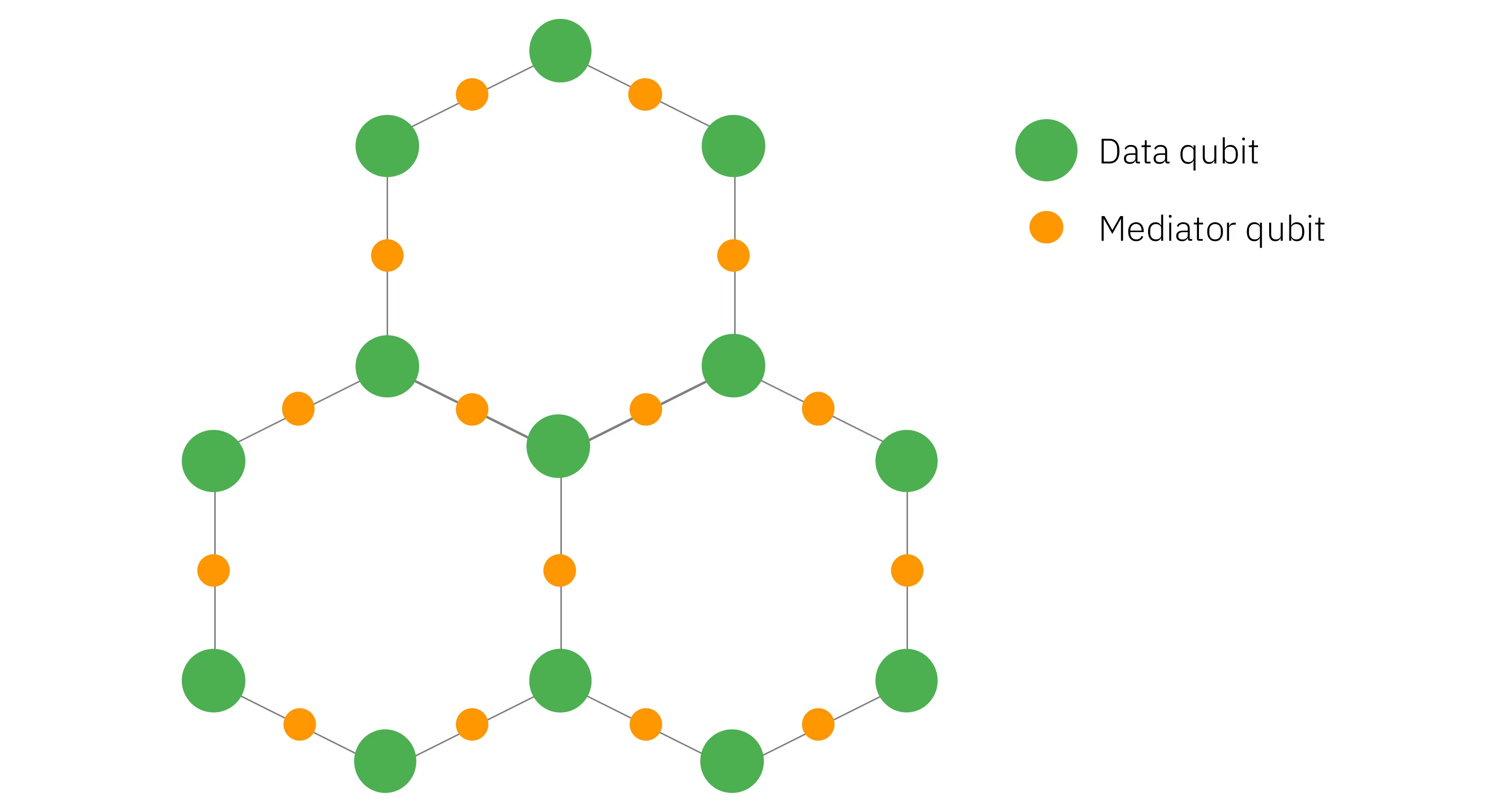
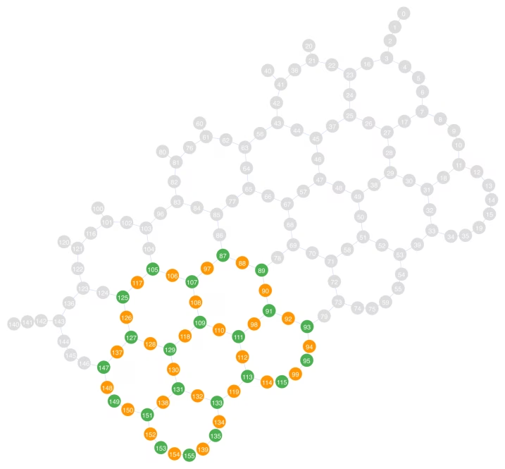
วงจรนี้จำลอง 4 ขั้นตอน Trotter ของ Hamiltonian แบบ transverse-field Ising ขนาด 22 qubit บนโครงตาข่ายหกเหลี่ยม data qubit ทั้ง 22 ตัวถูกฝังอยู่ใน heavy-hex subgraph ขนาด 49 qubit ของ QPU Heron r3 ที่ชื่อ ibm_boston ancilla qubit ทั้ง 27 ตัวถูกใช้เพื่อวัตถุประสงค์สองอย่าง คือการเป็นตัวกลางการพัวพันระหว่าง Ising qubit และการตรวจจับข้อผิดพลาดเชิงตรรกะระหว่างการรันวงจร เลเยอร์การพัวพันของวงจรถูกสร้างขึ้นเพื่อให้ mediator qubit กลับสู่สถานะพื้น $|0\rangle$ ก่อนการวัดครั้งสุดท้าย mediator qubit หนึ่งตัวหรือมากกว่าที่วัดได้ $|1\rangle$ แสดงว่าตัวอย่างนั้นเสียหายจากข้อผิดพลาดเชิงตรรกะ การตัดตัวอย่างเหล่านี้ทิ้งสามารถปรับปรุงความเที่ยงตรงของการกระจายตัวอย่างได้

ในกราฟด้านล่าง qubit สีเขียวแสดงถึง Ising qubit ทั้ง 22 ตัว และ qubit สีส้มแสดงถึง mediator qubit ทั้ง 27 ตัว

from qiskit.circuit import ClassicalRegister
from qiskit.transpiler import generate_preset_pass_manager
from qiskit_ibm_runtime import QiskitRuntimeService

backend_name = "ibm_boston"

def generate_ed_ising(graph, depth, zz_coeff, x_coeff):
    """Build the mediated error-detecting Ising circuit for data-qubit `graph`; returns (circuit, CZ layers, hardware graph)."""
    hw_graph = nx.Graph()
    for i, (a, b) in enumerate(graph.edges()):
        hw_graph.add_edges_from(
            [(a, i + graph.order()), (b, i + graph.order())]
        )
    coloring = nx.coloring.greedy_color(
        nx.line_graph(hw_graph), strategy="DSATUR"
    )
    layers_coupling = [
        [e for e, c in coloring.items() if c == i]
        for i in set(coloring.values())
    ]
    circuit = QuantumCircuit(hw_graph.order())
    circuit.h(range(hw_graph.order()))
    for _ in range(depth):
        for angle, qubits in (
            (zz_coeff, range(graph.order(), hw_graph.order())),
            (x_coeff, range(graph.order())),
        ):
            circuit.barrier()
            for layer in layers_coupling:
                for edge in layer:
                    circuit.cz(*edge)
            circuit.barrier()
            circuit.rx(angle, qubits)
    circuit.barrier()
    circuit.h(range(graph.order(), hw_graph.order()))
    return circuit, layers_coupling, hw_graph

service = QiskitRuntimeService()
backend = service.backend(backend_name)

circuit, layers_coupling, hw_graph = generate_ed_ising(
    data_graph, depth, zz_coeff, x_coeff
)

circ_meas = circuit.copy()
data_reg, check_reg = (
    ClassicalRegister(n_data, "data"),
    ClassicalRegister(n_checks, "check"),
)
circ_meas.add_register(data_reg, check_reg)
circ_meas.barrier()
circ_meas.measure(range(n_data), data_reg)
circ_meas.measure(range(n_data, n_qubits), check_reg)

# Physical qubits hosting the 22 Ising sites on ibm_boston, one heavy-hex row per lattice chain;
# the mediator for each edge is the physical qubit sitting between its two data qubits
data_layout = [
    *[95, 93, 91, 89, 87],
    *[115, 113, 111, 109, 107, 105],
    *[135, 133, 131, 129, 127, 125],
    *[155, 153, 151, 149, 147],
]
coupling_graph = nx.Graph(list(backend.coupling_map.get_edges()))
layout = data_layout + [
    next(
        iter(
            nx.common_neighbors(
                coupling_graph, data_layout[a], data_layout[b]
            )
        )
    )
    for a, b in data_graph.edges()
]

circ_trans = generate_preset_pass_manager(
    backend=backend, optimization_level=1, initial_layout=layout
).run(circ_meas)

plot_layout(backend, layout, n_data)

ระบุเลเยอร์การพัวพันในวงจรด้วย samplomatic

pass generate_boxing_pass_manager ของ Samplomatic จัดกลุ่มเลเยอร์การพัวพันของวงจรเป็นกล่องที่มีคำอธิบายประกอบสำหรับ Pauli twirling และการฉีดสัญญาณรบกวนแบบ PEC วงจรแม่แบบและ samplex ที่ได้ (การกระจายเชิงพารามิเตอร์บนวงจรแม่แบบที่ระบุ twirl และการฉีดสัญญาณรบกวน) ถูกใช้เพื่อกำหนดและรันการทดลอง QPU สำหรับการเรียนรู้สัญญาณรบกวนและการสุ่มตัวอย่างทั้งหมด กล่องการวัดยังมีคำอธิบายประกอบ ChangeBasis ด้วย ดังนั้นการหมุนที่วัด data qubit ในฐาน X จึงถูกส่งให้ samplex เป็นอินพุตในขณะสุ่มตัวอย่าง แทนที่จะฝังไว้ในวงจร

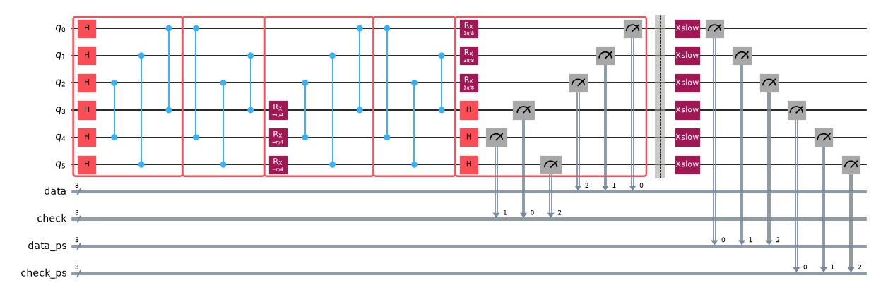
ด้านล่างนี้ boxing pass เดียวกันถูกนำไปใช้กับวงจร Ising ที่ตรวจจับข้อผิดพลาดในเวอร์ชันเล็ก เพื่อให้เราสามารถแสดงภาพโครงสร้างของวงจรที่ถูกจัดกล่องได้

from samplomatic.builders import build
from samplomatic.transpiler import generate_boxing_pass_manager
from samplomatic.utils import find_unique_box_instructions

boxed = generate_boxing_pass_manager(
    enable_gates=True,
    enable_measures=True,
    inject_noise_targets="gates",
    inject_noise_strategy="individual_modification",
    inject_noise_site="after",
    twirling_strategy="active_circuit",
    measure_annotations="all",
).run(circ_trans)
template, samplex = build(boxed)
unique_instructions = find_unique_box_instructions(
    boxed, normalize_annotations=None, undress_boxes=True
)

# Measure X on the data qubits and Z on the mediators
basis_key = next(
    s.name
    for s in samplex.inputs().get_specs()
    if s.name.startswith("basis_changes.")
)
meas_basis = np.array(
    [2 if q in set(layout[:n_data]) else 1 for q in sorted(layout)],
    dtype=np.uint8,
)

draw_toy_circuit(generate_ed_ising, zz_coeff, x_coeff, include_checks=False)

เพิ่มการตรวจสอบข้อผิดพลาดแบบ non-Markovian ให้กับวงจร

ถัดไป เราเพิ่มการตรวจสอบข้อผิดพลาดแบบ non-Markovian ให้กับ Circuit เพื่อป้องกันสัญญาณรบกวนที่ไม่ได้ถูกจำลองไว้ในโพรโทคอลการเรียนรู้ของเรา การตรวจสอบเหล่านี้ทำงานโดยการสร้าง bit-flip แบบพัลส์ยาวและตรวจสอบว่า qubit เคลื่อนที่จากสถานะคลาสสิกหนึ่งไปยังอีกสถานะหนึ่งอย่างถูกต้อง หาก qubit ทั้งสองตัวบนขอบใดขอบหนึ่งไม่ผ่านการตรวจสอบ ตัวอย่างนั้นจะถูกตัดทิ้ง การตรวจสอบข้อผิดพลาดแบบ non-Markovian สามารถใช้ที่จุดเริ่มต้นหรือจุดสิ้นสุดของ Circuit (หรือทั้งสองจุด) โดยในที่นี้เราใช้เฉพาะที่จุดสิ้นสุดเท่านั้น เรายังวางการตรวจสอบไว้บน spectator qubit ที่ไม่ได้ใช้งานซึ่งอยู่ติดกับ Circuit เพื่อให้ครอบคลุมสัญญาณรบกวนที่การตรวจสอบเหล่านี้ถูกออกแบบมาให้ตรวจจับได้มากขึ้น

โปรดจำไว้ว่า เช่นเดียวกับการตรวจสอบสมมาตร นี่ก็เป็นรูปแบบหนึ่งของ postselection เช่นกัน ดังนั้นเราจึงต้องแน่ใจว่าได้คำนึงถึงอัตรา postselection ที่ลดลง เมื่อผสานเทคนิคเหล่านี้เข้าด้วยกัน โดยเฉพาะ หาก $P(\text{non-Markovian error}) = \alpha$ และ $P(\text{symmetry error}) = \beta$ แล้วคุณจะต้องใช้ตัวอย่างที่มีสัญญาณรบกวนประมาณ $\frac{1}{(1-\alpha)(1-\beta)}$ ตัวอย่างเพื่อกู้คืนตัวอย่างเชิงตรรกะหนึ่งตัวอย่าง

from qiskit.transpiler import PassManager
from qiskit_mitigation.postselection import PostSelector
from qiskit_mitigation.postselection.passes import (
    AddPostCircuitNonMarkovianErrorChecks,
    AddSpectatorPostCircuitNonMarkovianErrorChecks,
)

add_checks = PassManager(
    [
        AddPostCircuitNonMarkovianErrorChecks(x_pulse_type="xslow"),
        AddSpectatorPostCircuitNonMarkovianErrorChecks(
            backend.coupling_map, x_pulse_type="xslow"
        ),
    ]
)
template_checked = add_checks.run(template)
selector = PostSelector.from_circuit(template_checked, backend.coupling_map)

draw_toy_circuit(generate_ed_ising, zz_coeff, x_coeff, include_checks=True)

เรียนรู้สัญญาณรบกวนของ gate และการอ่านค่าสำหรับวงจร checked-Ising ขนาด 49 qubit

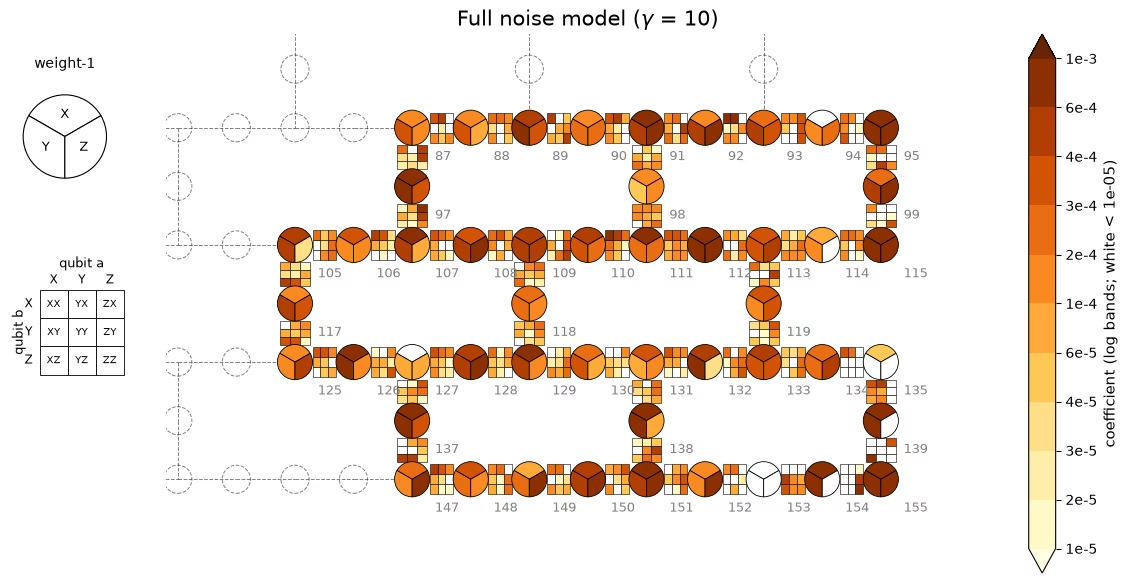
เพื่อลดสัญญาณรบกวน เราต้องจำลองว่าสัญญาณรบกวนส่งผลต่อ gate การพัวพันของเราอย่างไร ในที่นี้เราเรียนรู้โมเดลสัญญาณรบกวนแบบ Pauli-Lindblad สำหรับแต่ละเลเยอร์การพัวพันที่ไม่ซ้ำกันสามเลเยอร์ของวงจรโดยใช้ qiskit-noise-learning ต่อมา เราจะตัดพจน์ error generator ที่สามารถตรวจพบได้ด้วยการตรวจสอบสมมาตรออกจากโมเดลสัญญาณรบกวนนี้ และลดสัญญาณรบกวนเฉพาะช่องที่เหลือด้วย PEC แผนที่ด้านล่างแสดงเลเยอร์ที่เรียนรู้แล้วทั้งสามเลเยอร์บน QPU โดยแต่ละ qubit เป็นวงล้อของอัตรา weight-1 X/Y/Z และแต่ละ coupler เป็นตารางขนาด 3×3 ของอัตรา Pauli แบบ weight-2 บนคู่นั้น ค่า $\gamma$ เท่ากับ $10$ หมายถึงต้นทุนการสุ่มตัวอย่าง $\gamma^2=10^2=100$

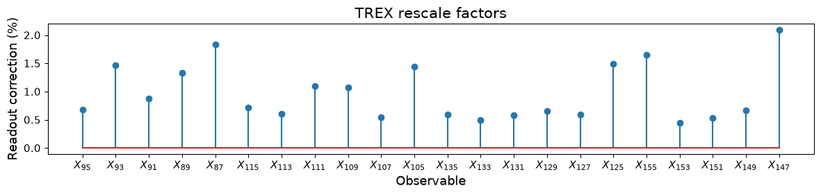
การแก้ไขการอ่านค่า (TREX) มาจากเส้นทาง SPAM ของการฟิตการเรียนรู้สัญญาณรบกวนโดยตรง กราฟก้าน (stem plot) ด้านล่างแผนที่สัญญาณรบกวนของ QPU แสดงตัวคูณปรับสเกล TREX ต่อ observable แต่ละตัว

from qiskit.quantum_info import PauliLindbladMap, QubitSparsePauli
from qiskit_ibm_runtime import Executor, Session
from qiskit_ibm_runtime.quantum_program import QuantumProgram
from qiskit_mitigation.trex import TREX
from qiskit_noise_learning.analysis import (
    ComputeObservables,
    CurveFitObservables,
    FlipPostSelect,
    LeastSquaresSolve,
)
from qiskit_noise_learning.circuit_generator import ExecutorCircuitGenerator
from qiskit_noise_learning.experiment_builder import (
    BindFragmentDepths,
    CompleteSequences,
    EvenDepthVanillaPaths,
    Experiment,
    GenerateInstructionSequences,
    IdentifyRelations,
    MergeInstructionSequences,
    SPAMPaths,
    VanillaInstructionSequences,
)
from qiskit_noise_learning.gate_sets import QiskitGateSet
from qiskit_noise_learning.models import PauliLindbladModel
from qiskit_noise_learning.models.utils import split_pauli_lindblad_model
from samplomatic.annotations import InjectNoise
from samplomatic.utils import get_annotation

gate_set = QiskitGateSet(
    target=backend.target,
    qubit_subset=sorted(
        {
            boxed.find_bit(q).index
            for i in unique_instructions
            for q in i.qubits
        }
    ),
)
ref_to_qubits = {}
for inst in unique_instructions:
    if ann := get_annotation(inst.operation, InjectNoise):
        gate_set.add_box_as_gate(inst, name=ann.ref)
        ref_to_qubits[ann.ref] = sorted(
            boxed.find_bit(q).index for q in inst.qubits
        )

fidelity_model = PauliLindbladModel.k_local(
    gate_set, gate_k={**{r: 2 for r in ref_to_qubits}, "M": 1, "P": 1}
)
experiment = (
    EvenDepthVanillaPaths()
    + VanillaInstructionSequences()
    + IdentifyRelations()
    + SPAMPaths()
    + GenerateInstructionSequences()
    + MergeInstructionSequences()
    + CompleteSequences()
    + BindFragmentDepths([2, 4, 8, 12])
).run(Experiment(fidelity_model=fidelity_model, shots=384, randomizations=64))

circuit_generator = ExecutorCircuitGenerator(
    gate_set, pass_manager=add_checks
)
program_learn, data_mapper = circuit_generator.generate(experiment)

session = Session(backend)
executor_options = {"environment": {"job_tags": ["TUT_PECLNM"]}}
fit = circuit_generator.collect(
    Executor(session, options=executor_options).run(program_learn).result(),
    data_mapper,
)
fit = (
    FlipPostSelect()
    + ComputeObservables()
    + CurveFitObservables()
    + LeastSquaresSolve()
).run(fit)
print(
    "learning shots removed by checks:",
    f"{float(fit.raw_data.datatree['0']['data_mask'].mean()):.4f}",
)

# TREX factors from the fit's SPAM paths: the fit only identifies the product of
# state-prep and measurement error, so hand TREX the composition of the two maps
spam = fidelity_model.to_pauli_lindblad_maps(
    fit.model_data, include_spam=True
)
spam_map = spam["P"].compose(spam["M"])
z_terms = [
    QubitSparsePauli(("Z", [layout[i]]), num_qubits=backend.num_qubits)
    for i in range(n_data)
]
trex_rescale = np.array(
    [TREX.calculate_trex_factor(spam_map, z) for z in z_terms]
)

# learned maps come back in backend qubit indexing; samplex wants box-local order
plm = split_pauli_lindblad_model(fit.model).model
noise_maps = {}
for ref, m in plm.to_pauli_lindblad_maps(fit.model_data).items():
    box = ref_to_qubits[ref]
    noise_maps[ref] = PauliLindbladMap.from_sparse_list(
        [
            (p, tuple(box.index(q) for q in qs), r)
            for p, qs, r in m.to_sparse_list()
        ],
        num_qubits=len(box),
    )
# Full-PEC cost: each learned layer acts twice per Trotter step (compute + uncompute)
gamma = float(
    np.exp(2 * depth * sum(2 * sum(m.rates) for m in noise_maps.values()))
)

# Collect the learned model in the form the figure helpers expect
mit = dict(
    **{
        f"rates_{i}": np.asarray(m.rates)
        for i, m in enumerate(noise_maps.values())
    },
    **{
        f"label_paulis_{i}": np.array([p for p, _, _ in m.to_sparse_list()])
        for i, m in enumerate(noise_maps.values())
    },
    **{
        f"label_qubits_{i}": np.array(
            [
                list(qs) + [-1] * (2 - len(qs))
                for _, qs, _ in m.to_sparse_list()
            ]
        )
        for i, m in enumerate(noise_maps.values())
    },
    layout=np.array(layout),
    trex_rescale=trex_rescale,
    gammas=np.array([gamma, np.nan]),
)
draw_noise_map(mit, backend)
plot_trex(mit["trex_rescale"], x_labels(layout, n_data))

learning shots removed by checks: 0.2393

ตัดพจน์ที่ตรวจพบได้ด้วยการตรวจสอบสมมาตรออกจากโมเดลสัญญาณรบกวน

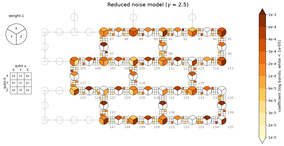
การตรวจสอบสมมาตรแต่ละแบบสามารถตรวจจับ error generator บางส่วนในโมเดลสัญญาณรบกวนได้ ซึ่งหมายความว่าคุณไม่จำเป็นต้องลดข้อผิดพลาดเหล่านั้น ในที่นี้เราสร้างมาสก์เหนือ noise generator ที่ตรวจจับได้โดยใช้ฟังก์ชัน create_postselected_noise_mask จาก qiskit_mitigation มาสก์นี้จะถูกใช้เพื่อตัดพจน์ที่ตรวจจับได้ออกจากโมเดลสัญญาณรบกวนก่อนทำ PEC การทำ PEC โดยอ้างอิงกับโมเดลสัญญาณรบกวนที่ถูกตัดแล้วสามารถให้ค่าคาดหวังที่ลู่เข้าได้ด้วยต้นทุนการสุ่มตัวอย่างเพียงเสี้ยวหนึ่งของต้นทุนที่ต้องใช้ในการทำ PEC บนโมเดลสัญญาณรบกวนเต็มรูปแบบ ดังที่แสดงในแผนที่โมเดลสัญญาณรบกวนด้านบน

แผนที่ด้านล่างวาดด้วยสเกลสีเดียวกันกับโมเดลที่เรียนรู้แล้วด้านบน โดยเก็บไว้เฉพาะ error generator ที่การตรวจสอบไม่สามารถตรวจจับได้ เราเห็นว่า error generator จำนวนมากถูกลบออกจากโมเดล และต้นทุนการสุ่มตัวอย่างลดลงอย่างมาก ต้นทุนการสุ่มตัวอย่างในการรัน PEC บนโมเดลสัญญาณรบกวนที่ถูกตัดแล้วคือ $\gamma^2=2.5^2\approx6.3$ ซึ่งลดลงประมาณ 16 เท่าจากต้นทุนที่จำเป็นในการลดสัญญาณรบกวนช่องเต็มรูปแบบ

from qiskit.quantum_info import Pauli
from qiskit_mitigation.noise import create_postselected_noise_mask

SHOTS_PER_RAND = 64  # shots per PEC randomization
N_RAND = 23_054  # PEC randomizations per experiment
MAX_PAIR_RATE = 0.02  # Max value of any coupler's summed two-qubit error rate

# The detectors are virtual Pauli-Z's representing the measurements on the mediator qubits
# We can find the set of detectable noise generators in the model for each detector by conjugating
# it backward through the circuit and calculating what generators it anti-commutes with.
detectors = [
    Pauli("I" * (boxed.num_qubits - 1 - q) + "Z" + "I" * q)
    for q in layout[n_data:]
]
# Detectable generators are handled by postselection; prune them from the model for PEC
local_scales, gamma2_post = create_postselected_noise_mask(
    boxed, noise_maps, detectors
)
gamma_post = gamma2_post**0.5
print(f"gamma PEC {gamma:.2f} | gamma QED+PEC {gamma_post:.2f}")

# Kill the job if any coupler's summed rate exceeds MAX_PAIR_RATE
pair_lam = {}
for m in noise_maps.values():
    for _, qs, r in m.to_sparse_list():
        if len(qs) == 2:
            pair_lam[tuple(sorted(qs))] = (
                pair_lam.get(tuple(sorted(qs)), 0.0) + r
            )
assert (
    max(pair_lam.values()) < MAX_PAIR_RATE
), f"kill: degraded coupler {max(pair_lam, key=pair_lam.get)}"

# Detectability depends on circuit position, so record each site's 0/1 scales by layer
site_ref = {
    a.modifier_ref: a.ref
    for inst in boxed.data
    if inst.operation.name == "box"
    and (a := get_annotation(inst.operation, InjectNoise))
    and a.ref
}
sites = sorted(local_scales, key=lambda s: int(s[1:]))
mit["site_scales"] = np.stack([local_scales[s] for s in sites])
mit["site_layer"] = np.array(
    [list(noise_maps).index(site_ref[s]) for s in sites]
)
mit["gammas"] = np.array([gamma, gamma_post])
draw_noise_map(mit, backend, reduced=True)

gamma PEC 10.08 | gamma QED+PEC 2.52

สุ่มตัวอย่างวงจรที่ตรวจจับข้อผิดพลาด

ในที่นี้เราสุ่มตัวอย่างวงจร Ising ที่ตรวจจับข้อผิดพลาดขนาด 49 qubit เราเปิดใช้งาน Pauli twirling และการตรวจสอบข้อผิดพลาดแบบ non-Markovian แต่เราไม่ทำการสุ่มตัวอย่างแบบ PEC เราจะใช้ตัวอย่างเหล่านี้ในการคำนวณค่าคาดหวังพื้นฐานรวมถึงค่าคาดหวังแบบใช้ error detection เพียงอย่างเดียว

# Baseline = the ED+PEC template itself at noise scale 0, i.e. twirling only
program_tw = QuantumProgram(shots=100)
program_tw.append_samplex_item(
    template_checked,
    samplex=samplex,
    shape=(1000, 1),
    samplex_arguments={
        "pauli_lindblad_maps": dict(noise_maps),
        basis_key: meas_basis,
        **{f"noise_scales.{k}": 0.0 for k in local_scales},
    },
)
job_tw = Executor(session, options=executor_options).run(program_tw)

สุ่มตัวอย่างวงจรที่ตรวจจับข้อผิดพลาดด้วย PEC

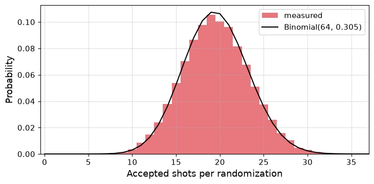
ตอนนี้เราสุ่มตัวอย่างอีกครั้งและรวม PEC randomization เข้าไปเพื่อลดสัญญาณรบกวนที่การตรวจสอบสมมาตรไม่สามารถตรวจจับได้ ตัวอย่างเหล่านี้จะถูกใช้ในการคำนวณค่าคาดหวังโดยใช้ error detection ร่วมกับ PEC ด้านล่างนี้เราพลอตจำนวนช็อตที่ยอมรับต่อ PEC randomization เทียบกับการแจกแจงทวินามที่อัตราการยอมรับเฉลี่ย เราเห็นว่าการยอมรับไม่มีความสัมพันธ์กับอินสแตนซ์วงจรที่สุ่มตัวอย่าง เนื่องจาก QED+PEC ฉีดเฉพาะ Pauli ที่ตรวจจับไม่ได้ ซึ่งสลับที่ได้กับการวัดของ mediator qubit ทุกตัว

def launch(session, template, samplex, samplex_args, n_rand, shots_per_rand):
    """Sample `n_rand` randomizations of `template` on `session` in <=100k-randomization jobs; returns the jobs."""
    jobs = []
    for start in range(0, n_rand, 100_000):
        program = QuantumProgram(shots=shots_per_rand)
        program.append_samplex_item(
            template,
            samplex=samplex,
            samplex_arguments=samplex_args,
            shape=(min(100_000, n_rand - start), 1),
        )
        jobs.append(Executor(session, options=executor_options).run(program))
    return jobs

# Reduced PEC
args_post = {
    "pauli_lindblad_maps": dict(noise_maps),
    basis_key: meas_basis,
    **{f"noise_scales.{k}": -1.0 for k in local_scales},
    **{f"local_scales.{k}": v for k, v in local_scales.items()},
}
# PEC on the full noise model
args_van = {
    "pauli_lindblad_maps": dict(noise_maps),
    basis_key: meas_basis,
    **{f"noise_scales.{k}": -1.0 for k in local_scales},
}

# Run sampling jobs
jobs = launch(
    session, template_checked, samplex, args_post, N_RAND, SHOTS_PER_RAND
)
jobs_van = launch(
    session, template_checked, samplex, args_van, N_RAND, SHOTS_PER_RAND
)
outs = [j.result()[0] for j in jobs]
outs_van = [j.result()[0] for j in jobs_van]
(out_tw,) = job_tw.result()
session.close()

รวบรวมตัวอย่างและตรวจสอบว่า PEC randomization สลับที่ได้กับการวัดบน mediator qubit และไม่ส่งผลต่อสถิติของ postselection

def bitflip_mask(out, selector):
    """Per-shot True/False for job result `out`: shot passes `selector`'s non-Markovian error checks."""
    regs = {
        k: np.asarray(out[k])
        for k in out
        if not k.startswith(("measurement_flips", "pauli_signs"))
    }
    return selector.compute_mask(regs, "edge", mode="post")

def symmetry_mask(out):
    """Per-shot True/False for job result `out`: every twirl-corrected symmetry check reads 0."""
    return ~(
        np.asarray(out["check"]) ^ np.asarray(out["measurement_flips.check"])
    ).any(axis=-1)

def keep_mask(out, selector):
    """Per-shot True/False for job result `out`: shot passes both check types."""
    return symmetry_mask(out) & bitflip_mask(out, selector)

def fracs(out_list, selector):
    """Fractions of shots across the job results in `out_list` passing [no, non-Markovian error, symmetry, both] checks."""
    bf = np.concatenate([bitflip_mask(o, selector) for o in out_list])
    sy = np.concatenate([symmetry_mask(o) for o in out_list])
    return [1.0, bf.mean(), sy.mean(), (bf & sy).mean()]

mask_post = np.concatenate([keep_mask(o, selector) for o in outs])

# Collect the sampled data alongside the learned model, in the form the figure helpers expect
mit.update(
    ps_fracs=np.array(
        [
            fracs([out_tw], selector),
            fracs(outs_van, selector),
            fracs(outs, selector),
        ]
    ),
    acc_counts_post=np.squeeze(mask_post).sum(axis=-1),
    data_tw=np.asarray(out_tw["data"]),
    flips_tw=np.asarray(out_tw["measurement_flips.data"]),
    mask_tw=keep_mask(out_tw, selector),
    data_post=np.packbits(
        np.concatenate([np.asarray(o["data"]) for o in outs]), axis=-1
    ),
    flips_post=np.concatenate(
        [np.asarray(o["measurement_flips.data"]) for o in outs]
    ),
    signs_post=np.concatenate([np.asarray(o["pauli_signs"]) for o in outs]),
    mask_post=mask_post,
    data_van=np.packbits(
        np.concatenate([np.asarray(o["data"]) for o in outs_van]), axis=-1
    ),
    flips_van=np.concatenate(
        [np.asarray(o["measurement_flips.data"]) for o in outs_van]
    ),
    signs_van=np.concatenate(
        [np.asarray(o["pauli_signs"]) for o in outs_van]
    ),
    mask_van=np.concatenate([bitflip_mask(o, selector) for o in outs_van]),
)

# Plot the PEC bias check
plot_postselection(mit)

คำนวณค่าคาดหวังและเปรียบเทียบกลยุทธ์

สุดท้าย เราคำนวณค่าคาดหวังทั้งหมดด้วยฟังก์ชันช่วยเหลือ executor_expectation_values จาก qiskit-mitigation ซึ่งจะใช้ measurement flip, มาสก์ postselection, ตัวคูณปรับสเกล TREX และเครื่องหมายของ quasi-probability ให้เราโดยอัตโนมัติ

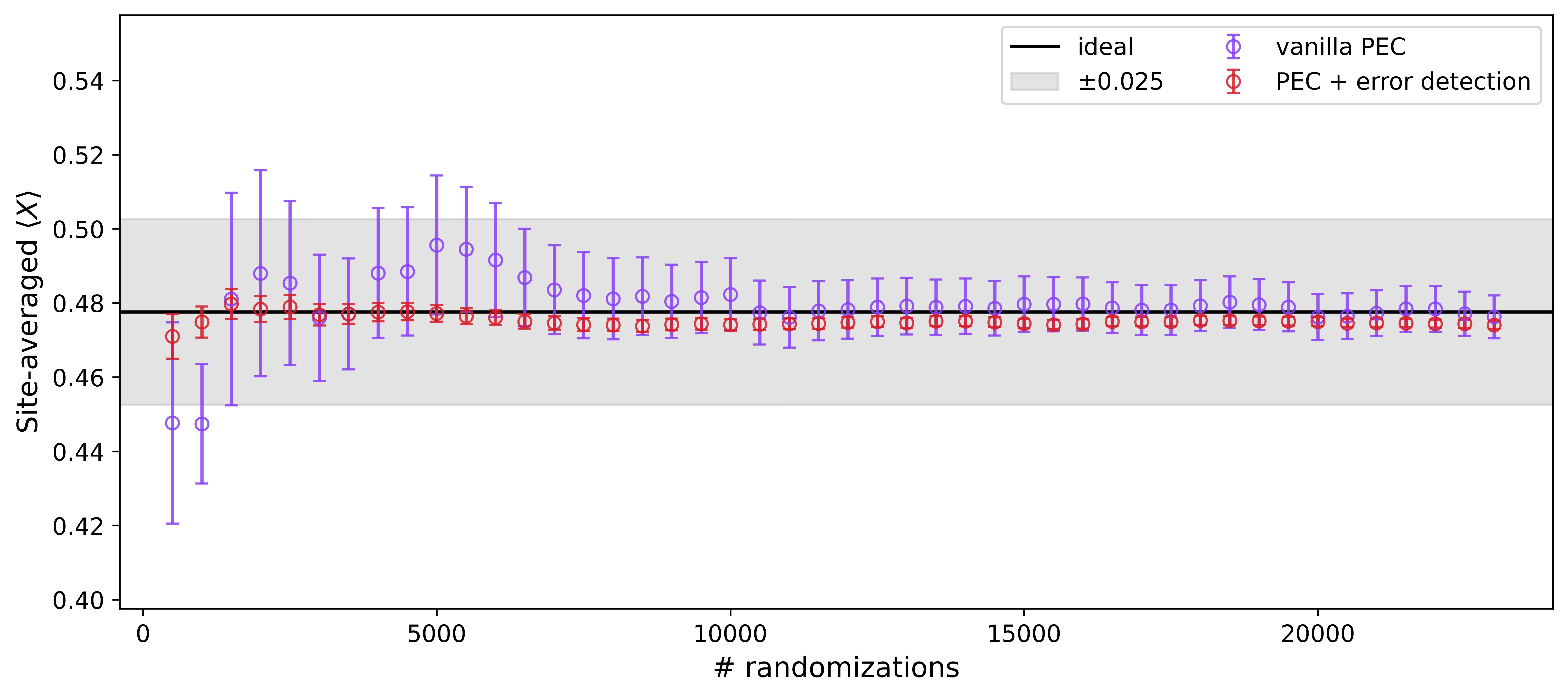
กราฟด้านบน: เราเห็นว่า PEC ทั้งสองรูปแบบลู่เข้า แต่ QED+PEC เข้าสู่แถบ $\pm 0.025$ ได้ด้วย randomization ที่น้อยกว่าและแถบข้อผิดพลาดที่แคบกว่า ความเอนเอียงที่เหลืออยู่ในการคำนวณ QED+PEC ต่ำกว่า 0.01 และอาจมาจากการรวมกันของความไม่ตรงกันของโมเดลสัญญาณรบกวน การเลื่อนของ qubit ตามเวลา และผลจากแหล่งสัญญาณรบกวนที่ไม่ได้ถูกจำลองไว้

กราฟด้านล่าง: ค่าประมาณสะสมของ $\langle X \rangle$ ที่เฉลี่ยตามไซต์ เมื่อ randomization สะสมขึ้นโดยใช้จำนวนช็อตต่อ randomization เท่ากันสำหรับ PEC ทั้งสองรูปแบบ PEC + การตรวจจับข้อผิดพลาด เข้าสู่แถบภายใน randomization ไม่กี่พันครั้ง ในขณะที่ PEC เพียงอย่างเดียว ซึ่งต้องจ่ายต้นทุนการสุ่มตัวอย่างเต็มรูปแบบ ต้องใช้ randomization มากกว่ามากจึงจะลู่เข้า

from qiskit.quantum_info import SparsePauliOp
from qiskit_mitigation.utils import executor_expectation_values

gamma, gamma_post = mit["gammas"]
basis_map = {Pauli("X" * n_data): [SparsePauliOp(o) for o in observables]}
rescale = dict(zip(observables, mit["trex_rescale"], strict=True))

def evs(bits, basis_map, **kwargs):
    """Per-site (means, standard errors) from boolean shot data `bits` of shape (rands, 1, shots, n_data)."""
    out = executor_expectation_values(
        bits, basis_map, None, avg_axis=(0, 1), **kwargs
    )
    return np.array([m for m, _ in out]).ravel(), np.sqrt(
        [v for _, v in out]
    ).ravel()

def unpack(mit, prefix, n_data):
    """Restore `mit[f"data_\{prefix\}"]` from packed bytes to booleans of shape (rands, 1, shots, n_data)."""
    return np.unpackbits(mit[f"data_{prefix}"], axis=-1)[..., :n_data].astype(
        bool
    )

unmit_tw, unmit_tw_err = evs(
    mit["data_tw"], basis_map, measurement_flips=mit["flips_tw"]
)
ed_tw, ed_tw_err = evs(
    mit["data_tw"],
    basis_map,
    measurement_flips=mit["flips_tw"],
    postselect_mask=mit["mask_tw"],
    rescale_factors=rescale,
)
post, post_err = evs(
    unpack(mit, "post", n_data),
    basis_map,
    measurement_flips=mit["flips_post"],
    pauli_signs=mit["signs_post"],
    postselect_mask=mit["mask_post"],
    rescale_factors=rescale,
)
pec, pec_err = evs(
    unpack(mit, "van", n_data),
    basis_map,
    measurement_flips=mit["flips_van"],
    pauli_signs=mit["signs_van"],
    postselect_mask=mit["mask_van"],
    rescale_factors=rescale,
)

# effective ED+PEC overhead measured from the data: accepted shots per signed accepted shot
signs_post = 1 - 2 * (np.squeeze(mit["signs_post"]).sum(axis=-1) % 2)
gamma_eff = (
    mit["mask_post"].sum()
    / (signs_post * np.squeeze(mit["mask_post"]).sum(axis=-1)).sum()
)

print(
    f"gamma PEC {gamma:.2f} | gamma QED+PEC {gamma_post:.2f} (model) / {gamma_eff:.2f} (data) | "
    f"QED survival {mit['mask_tw'].mean():.3f} | QED+PEC survival {mit['mask_post'].mean():.3f} | "
    f"mean QED+PEC err {post_err.mean():.4f}"
)
plot_final(
    obs_exact,
    (unmit_tw, unmit_tw_err),
    (ed_tw, ed_tw_err),
    (pec, pec_err),
    (post, post_err),
    (gamma, gamma_post),
    x_labels(layout, n_data),
    "",
)

gamma PEC 10.08 | gamma QED+PEC 2.52 (model) / 2.51 (data) | QED survival 0.304 | QED+PEC survival 0.305 | mean QED+PEC err 0.0037

plot_convergence(mit, obs_exact, n_data)