Repetition codes
ประมาณการการใช้งาน: ไม่ถึง 10 วินาทีบนโปรเซสเซอร์ Heron (หมายเหตุ: นี่เป็นเพียงการประมาณเท่านั้น เวลาจริงอาจแตกต่างออกไป)
ผลลัพธ์การเรียนรู้
-
วิธีการติดตั้งรหัสแก้ไขความผิดพลาดแบบ bit-flip โดยใช้ Circuit แบบไดนามิก
-
วิธีการวัด stabilizer เพื่อตรวจจับความผิดพลาดควอนตัมโดยไม่ทำลายข้อมูลที่เข้ารหัสไว้
-
วิธีการประเมินประสิทธิภาพของการแก้ไขความผิดพลาดควอนตัมโดยเปรียบเทียบผลลัพธ์ที่แก้ไขแล้วและยังไม่ได้แก้ไข
ข้อกำหนดเบื้องต้น
พื้นหลัง
เพื่อให้สามารถแก้ไขข้อผิดพลาดควอนตัม (QEC) แบบเรียลไทม์ได้ คุณจำเป็นต้องควบคุมการไหลของโปรแกรมควอนตัมแบบไดนามิกระหว่างการรัน เพื่อให้ quantum gates สามารถทำงานตามเงื่อนไขของผลการวัดได้ บทแนะนำนี้รัน bit-flip code ซึ่งเป็นรูปแบบ QEC ที่เรียบง่ายมาก โดยแสดงให้เห็น dynamic quantum circuit ที่สามารถป้องกัน qubit ที่เข้ารหัสไว้จากข้อผิดพลาด bit-flip เดี่ยว และประเมินประสิทธิภาพของ bit-flip code
คุณสามารถใช้ประโยชน์จาก ancilla qubits เพิ่มเติมและ entanglement เพื่อวัด stabilizers ที่ไม่เปลี่ยนแปลงข้อมูลควอนตัมที่เข้ารหัสไว้ ขณะที่ยังคงบอกให้คุณทราบถึงข้อผิดพลาดบางประเภทที่อาจเกิดขึ้น quantum stabilizer code เข้ารหัส logical qubits ลงใน physical qubits Stabilizer codes มุ่งเน้นอย่างเฉพาะเจาะจงในการแก้ไขชุดข้อผิดพลาดแบบไม่ต่อเนื่องโดยอาศัย Pauli group
ในบทเรียนนี้ เราจะสาธิตรหัส bit-flip โดยใช้การทดลองหน่วยความจำควอนตัมอย่างง่าย เราจะเตรียมคิวบิตที่เข้ารหัสไว้ในสถานะลอจิคัล จากนั้นทำหลายรอบของช่วงเวลาว่าง (idle time) (เพื่อสะสมความผิดพลาด) ตามด้วยการตรวจจับและแก้ไขความผิดพลาด จากนั้นเราจะวัดปริมาณความน่าจะเป็นของความผิดพลาดเชิงลอจิคัลเป็นฟังก์ชันของจำนวนรอบ (เวลา) โดยความน่าจะเป็นของความผิดพลาดเชิงลอจิคัลคือความน่าจะเป็นที่จะพบคิวบิตอยู่ในสถานะที่ไม่กลับคืนสู่ หลังการวัดครั้งสุดท้าย (โดยเฉพาะ สถานะที่สอดคล้องกับความผิดพลาดคือ , , และ )
เราจะเปรียบเทียบอัตราความผิดพลาดเทียบกับเวลากับอัตราความผิดพลาดของคิวบิตเดี่ยวที่ไม่ได้เข้ารหัส และเปรียบเทียบกับการใช้รหัส repetition ที่เราตรวจจับและแก้ไขความผิดพลาดเฉพาะหลังการวัดครั้งสุดท้ายเท่านั้น แต่ไม่ใช่แบบไดนามิกระหว่าง Circuit
หมายเหตุ: รหัส repetition อนุญาตให้แก้ไขได้เฉพาะความผิดพลาดแบบ bit-flip เท่านั้น จึงไม่ใช่รหัสแก้ไขความผิดพลาดที่สมบูรณ์ อย่างไรก็ตาม เนื่องจากความเรียบง่ายของมัน จึงเป็นจุดเริ่มต้นที่ดีในการอธิบายวิธีการติดตั้งการแก้ไขความผิดพลาดบนคอมพิวเตอร์ควอนตัม การทดลองหน่วยความจำด้านล่างนี้ทดสอบเฉพาะความผิดพลาดประเภทเดียว (การสลายตัวของ ไปเป็น ) และในทางเทคนิคแสดงให้เห็นเพียงการปกป้องข้อมูลแบบคลาสสิกเท่านั้น
ข้อกำหนดเบื้องต้น
ก่อนเริ่มบทแนะนำนี้ ตรวจสอบให้แน่ใจว่าได้ติดตั้งสิ่งต่อไปนี้:
-
Qiskit SDK v2.0 หรือใหม่กว่า พร้อมการรองรับ visualization
-
Qiskit Runtime v0.40 หรือใหม่กว่า (
pip install qiskit-ibm-runtime)
การตั้งค่า
# Added by doQumentation — required packages for this notebook
!pip install -q matplotlib numpy qiskit qiskit-ibm-runtime scipy seaborn
import numpy as np
import seaborn as sns
import matplotlib.pyplot as plt
from scipy.optimize import curve_fit

sns.set()
plt.rc("xtick", labelsize=20)
plt.rc("ytick", labelsize=20)
plt.rc("lines", linewidth=3)
plt.rc("font", size=20)
plt.rc("legend", fontsize="large")
plt.rc("axes", labelsize=20)
plt.rcParams["figure.figsize"] = 15, 6
plt.rcParams["legend.title_fontsize"] = 25
# Qiskit imports
from qiskit import (
    QuantumCircuit,
    QuantumRegister,
    ClassicalRegister,
)

# qiskit-ibm-runtime
from qiskit_ibm_runtime import QiskitRuntimeService, SamplerV2 as Sampler
from qiskit_ibm_runtime.circuit import MidCircuitMeasure

service = QiskitRuntimeService()
ตัวอย่าง Simulator ขนาดเล็ก
เราจะข้ามขั้นตอนนี้ไป เนื่องจากเป้าหมายของการทดลองนี้คือการวัดอายุการใช้งาน (lifetime) ของคิวบิตเชิงลอจิคัลภายใต้สัญญาณรบกวนของฮาร์ดแวร์จริง เช่น amplitude damping ระหว่างดีเลย์ที่ว่างอยู่ Simulator ที่ไม่มีสัญญาณรบกวนจะไม่แสดงความผิดพลาดใด ๆ ให้ตรวจจับและแก้ไข
ตัวอย่างฮาร์ดแวร์ขนาดใหญ่
ขั้นตอนที่ 1 แปลง input แบบ classical เป็นปัญหาควอนตัม
เลือก Backend
เพื่อตรวจจับความผิดพลาดระหว่าง Circuit เราต้องเลือก Backend ที่สามารถเข้าถึงเมท็อด MidCircuitMeasure ได้ (ดู เอกสาร)
# You can see all backends that support mid-circuit measurements by running the following code.
service.backends(filters=lambda b: "measure_2" in b.supported_instructions)
[<IBMBackend('ibm_pittsburgh')>,
 <IBMBackend('ibm_boston')>,
 <IBMBackend('ibm_kingston')>]
# Choose the least busy backend that supports mid-circuit measurements (`measure_2`).

backend = service.least_busy(
    filters=lambda b: "measure_2" in b.supported_instructions,
    operational=True,
    simulator=False,
    dynamic_circuits=True,
)
# backend = service.backend(backend_name) # alternatively, you could choose a specific backend
print(backend.name)
ibm_boston
สร้างลำดับของ Circuit stabilizer แบบ bit-flip ที่ทำหลายรอบของการตรวจจับและแก้ไขความผิดพลาด
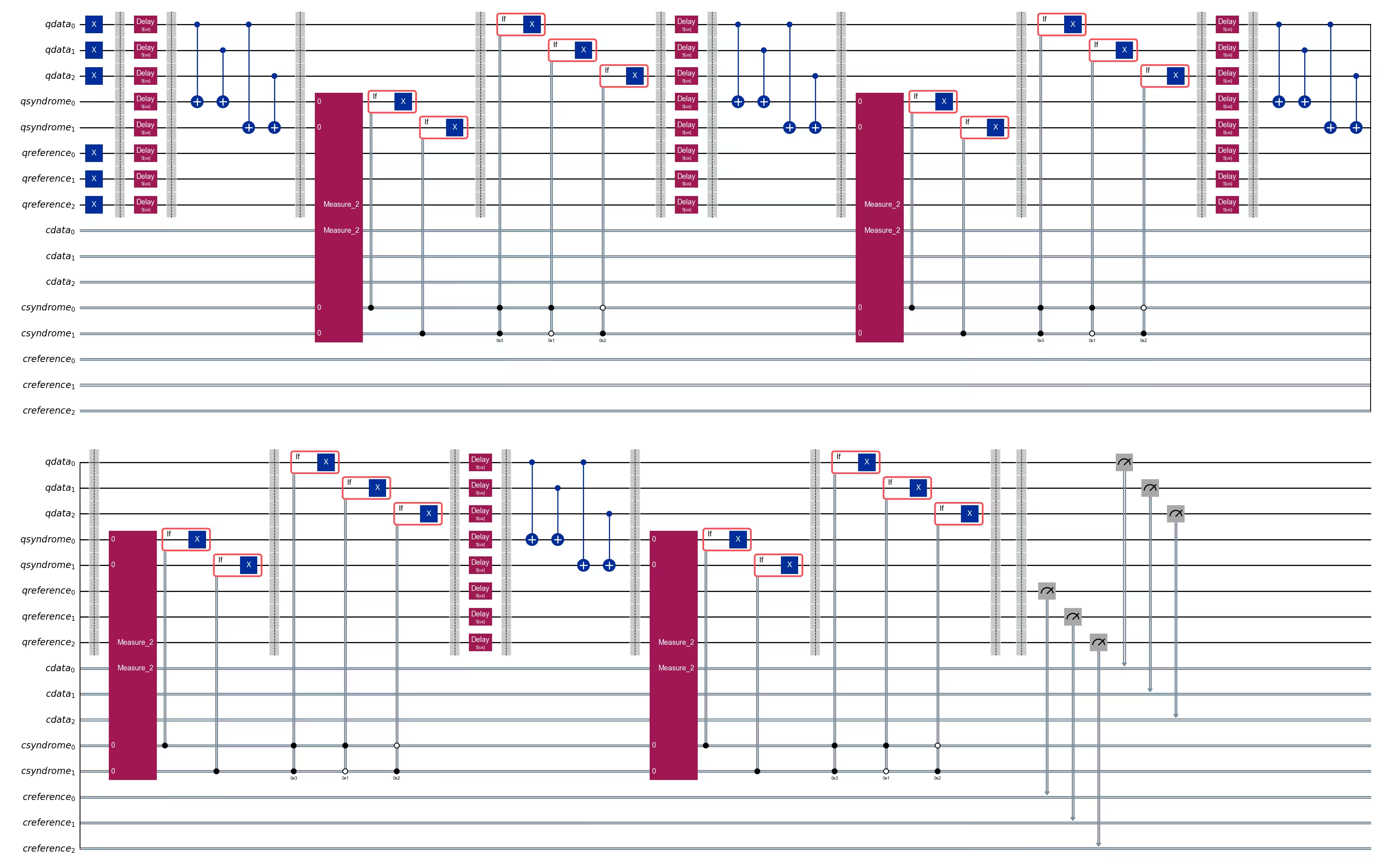
bit-flip code เป็นหนึ่งในตัวอย่างที่เรียบง่ายที่สุดของ stabilizer code โดยป้องกัน state จากข้อผิดพลาด bit-flip (X) เพียงครั้งเดียวบน qubit ใด ๆ ในการเข้ารหัส พิจารณาการทำงานของ bit-flip error ซึ่งแมป และ บน qubit ใด ๆ ของเรา จะได้ โค้ดนี้ต้องใช้ห้า qubit: สามตัวใช้เข้ารหัส state ที่ถูกป้องกัน และอีกสองตัวที่เหลือใช้เป็น ancilla สำหรับวัด stabilizer
ด้านล่างนี้คุณจะสร้าง Circuit ที่ (1) เตรียมคิวบิตข้อมูลในสถานะลอจิคัล จากนั้น (2) รันหลายรอบของดีเลย์ ตามด้วยการแก้ไขความผิดพลาด (รวมถึงการรีเซ็ตคิวบิต syndrome) และ (3) อ่านค่าสถานะของคิวบิตข้อมูล
เรายังจะทดสอบอายุการใช้งานของสถานะ โดยไม่ใช้การแก้ไขความผิดพลาด ด้วยการรวมคิวบิตอ้างอิงสามตัวที่เราเตรียมไว้ในสถานะ ปล่อยให้ว่าง แล้วอ่านค่าออกมา
def build_qc(
    qreg_data,
    qreg_syndrome,
    creg_data,
    creg_syndrome,
    qreg_ref=None,
    creg_ref=None,
):
    """Build a typical error correction circuit"""
    if qreg_ref:
        return QuantumCircuit(
            qreg_data,
            qreg_syndrome,
            creg_data,
            creg_syndrome,
            qreg_ref,
            creg_ref,
        )
    else:
        return QuantumCircuit(
            qreg_data, qreg_syndrome, creg_data, creg_syndrome
        )

def encode_bit_flip(circuit, qreg_data, qreg_ref=None) -> QuantumCircuit:
    """Encode bit-flip. This is done by simply adding a cx"""

    for q in qreg_data:
        circuit.x(q)

    if qreg_ref:
        for q in qreg_ref:
            circuit.x(q)

    circuit.barrier()

    return circuit

def measure_syndrome_bit(
    circuit, qreg_data, qreg_syndrome, creg_syndrome, qreg_ref=None
):
    """
    Measure the syndrome by measuring the parity.
    We reset our ancilla qubits after measuring the stabilizer
    so we can reuse them for repeated stabilizer measurements.
    Because we have already observed the state of the qubit,
    we can write the conditional reset protocol directly to
    avoid another round of qubit measurement if we used
    the `reset` instruction.
    """
    circuit.cx(qreg_data[0], qreg_syndrome[0])
    circuit.cx(qreg_data[1], qreg_syndrome[0])
    circuit.cx(qreg_data[0], qreg_syndrome[1])
    circuit.cx(qreg_data[2], qreg_syndrome[1])
    circuit.barrier()

    for q_measure, c_measure in zip(qreg_syndrome, creg_syndrome):
        circuit.append(MidCircuitMeasure(), [q_measure], [c_measure])

    with circuit.if_test((creg_syndrome[0], 1)):
        circuit.x(qreg_syndrome[0])
    with circuit.if_test((creg_syndrome[1], 1)):
        circuit.x(qreg_syndrome[1])

    circuit.barrier()
    return circuit

def apply_correction_bit(circuit, qreg_data, creg_syndrome):
    """We can detect where an error occurred and correct our state"""
    with circuit.if_test((creg_syndrome, 3)):
        circuit.x(qreg_data[0])
    with circuit.if_test((creg_syndrome, 1)):
        circuit.x(qreg_data[1])
    with circuit.if_test((creg_syndrome, 2)):
        circuit.x(qreg_data[2])
    circuit.barrier()
    return circuit

def apply_final_readout(
    circuit, qreg_data, creg_data, qreg_ref=None, creg_ref=None
):
    """Read out the final measurements"""

    circuit.barrier()
    if qreg_ref:
        circuit.measure(qreg_ref, creg_ref)
    circuit.measure(qreg_data, creg_data)

    return circuit
def build_error_correction_sequence(
    num_cycles, cycles_per_circuit, nq_ref=3, delay=None
) -> QuantumCircuit:
    circuits = []
    reps = []

    qreg_data = QuantumRegister(3, name="qdata")
    qreg_syndrome = QuantumRegister(2, name="qsyndrome")
    creg_data = ClassicalRegister(3, name="cdata")
    creg_syndrome = ClassicalRegister(2, name="csyndrome")
    qreg_ref = QuantumRegister(nq_ref, name="qreference")
    creg_ref = ClassicalRegister(nq_ref, name="creference")

    circuit = build_qc(
        qreg_data,
        qreg_syndrome,
        creg_data,
        creg_syndrome,
        qreg_ref=qreg_ref,
        creg_ref=creg_ref,
    )
    circuit = encode_bit_flip(circuit, qreg_data, qreg_ref=qreg_ref)

    circuit_n = circuit.copy()
    circuit_n = apply_final_readout(
        circuit_n, qreg_data, creg_data, qreg_ref=qreg_ref, creg_ref=creg_ref
    )
    circuits.append(circuit_n)
    reps.append(0)

    for i in range(1, num_cycles + 1):
        if delay:
            circuit.delay(delay, unit="us")
            circuit.barrier()
        circuit = measure_syndrome_bit(
            circuit,
            qreg_data,
            qreg_syndrome,
            creg_syndrome,
            qreg_ref=qreg_ref,
        )
        circuit = apply_correction_bit(circuit, qreg_data, creg_syndrome)
        circuit_n = circuit.copy()
        if i % cycles_per_circuit == 0:
            circuit_n = apply_final_readout(
                circuit_n,
                qreg_data,
                creg_data,
                qreg_ref=qreg_ref,
                creg_ref=creg_ref,
            )
            circuits.append(circuit_n)
            reps.append(i)

    return circuits, np.array(reps)

num_cycles = 40
cycles_per_circuit = 4
nq_ref = 3
circuits, rep_array = build_error_correction_sequence(
    num_cycles, cycles_per_circuit, nq_ref=3, delay=5
)
circuits[1].draw(output="mpl", cregbundle=False, fold=50)
ขั้นตอนที่ 2: ปรับแต่งปัญหาสำหรับการรันบนฮาร์ดแวร์ควอนตัม
เพื่อลดเวลาการรัน job โดยรวม Qiskit primitives รับเฉพาะ circuit และ observable ที่เป็นไปตามคำสั่งและการเชื่อมต่อที่ระบบเป้าหมายรองรับ (เรียกว่า ISA circuits และ observables) เรียนรู้เพิ่มเติมเกี่ยวกับการ transpile
สร้าง ISA circuits
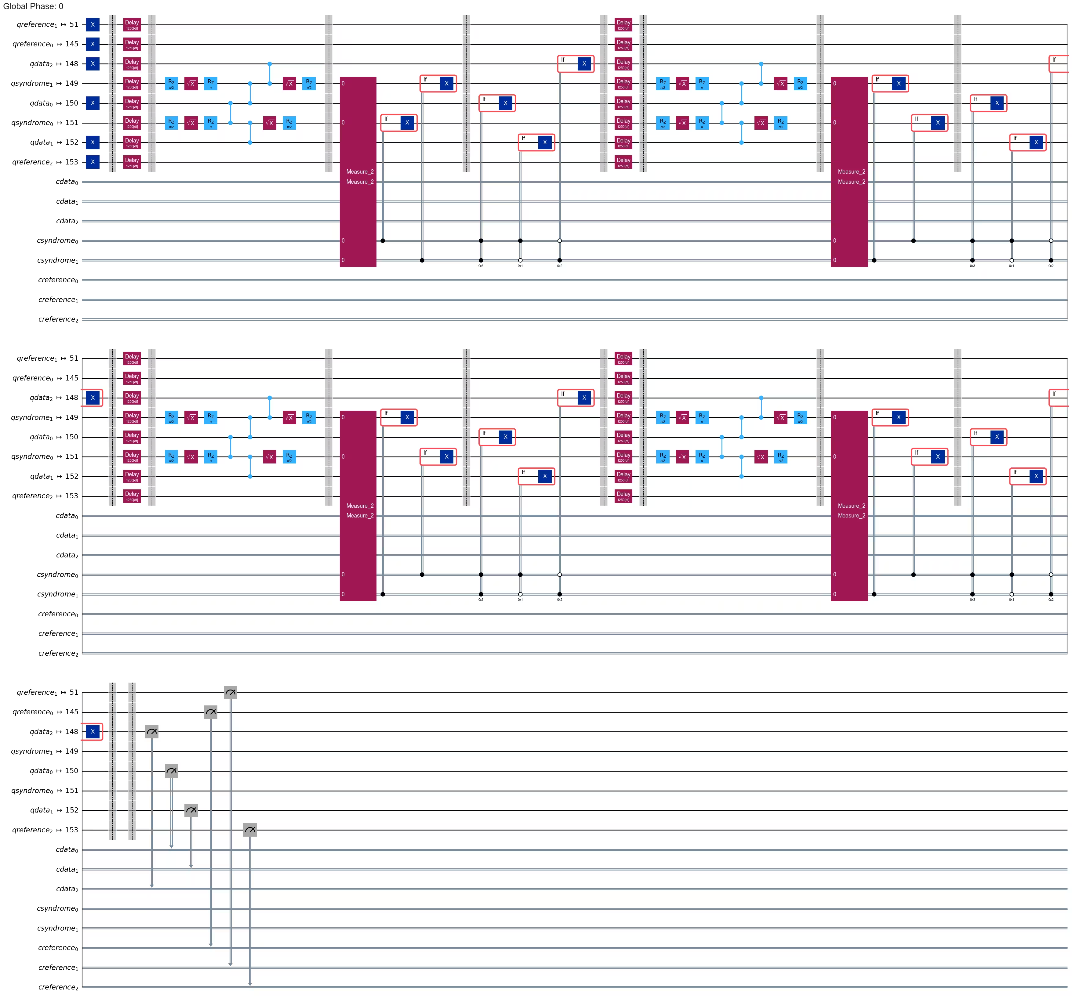
เราจะเริ่มด้วยการหา layout เริ่มต้น (นั่นคือ การเลือกคิวบิตทางกายภาพที่จะแมป Circuit ของเราลงไป) โดยการ transpile Circuit ที่ยาวที่สุดของเราด้วย preset pass manager ที่ optimization level 3
from qiskit.transpiler.preset_passmanagers import generate_preset_pass_manager

pm = generate_preset_pass_manager(backend=backend, optimization_level=3)
isa_circuit_ref = pm.run(circuits[-1])
init_layout = isa_circuit_ref.layout.initial_index_layout(
    filter_ancillas=True
)
print(init_layout)
[56, 44, 62, 43, 63, 22, 48, 67]
สำหรับคิวบิตอ้างอิงที่เราจะนำมาเปรียบเทียบกับหน่วยความจำควอนตัมเชิงลอจิคัลของเรา เราจะเลือกคิวบิตที่ดีที่สุดที่มีอยู่ในแง่ของเวลาความเชื่อมโยง (coherence time) จาก amplitude damping ()
# get all qubits ordered by T1
t1_data = []
for i in range(backend.num_qubits):
    try:
        t1_us = backend.properties().t1(i) * 1e6
    except Exception:
        t1_us = 0.0
    t1_data.append((i, t1_us))

t1_data_sorted = sorted(t1_data, key=lambda x: x[1], reverse=True)

# exclude the qubits we have already mapped the error correcting code to
t1_data_sorted = [
    t1_data for t1_data in t1_data_sorted if t1_data[0] not in init_layout[:5]
]

# use the best qubits in terms of T1 for the reference qubits
init_layout = init_layout[:5] + [t1_data[0] for t1_data in t1_data_sorted[:3]]
print(init_layout)
[56, 44, 62, 43, 63, 143, 131, 31]
# These are the resulting T1 times
properties = backend.properties()
print("Amplitude damping decoherence times for code data qubits:")
for q in init_layout[:3]:
    t1 = properties.t1(q)
    print(f"qubit {q}: T1 = {t1 * 1e6:.0f} mus")

print("\nAmplitude damping decoherence times for reference qubits:")
for q in init_layout[-3:]:
    t1 = properties.t1(q)
    print(f"qubit {q}: T1 = {t1 * 1e6:.0f} mus")
Amplitude damping decoherence times code data qubits:
qubit 56: T1 = 322 mus
qubit 44: T1 = 263 mus
qubit 62: T1 = 290 mus

Amplitude damping decoherence times reference qubits:
qubit 143: T1 = 442 mus
qubit 131: T1 = 410 mus
qubit 31: T1 = 401 mus
# now we transpile all circuits to this initial layout; this way each circuit is run on the same qubits and we can make a fair comparison
pm = generate_preset_pass_manager(
    backend=backend,
    optimization_level=3,
    initial_layout=init_layout,
)
isa_circuits = pm.run(circuits)
isa_circuits[1].draw("mpl", cregbundle=False, fold=50)
ขั้นตอนที่ 3 รันด้วย Qiskit primitives
sampler = Sampler(mode=backend)

sampler.options.environment.job_tags = ["TUT-REPCODE"]
sampler.options.max_execution_time = 600  # this workload is expected to be under 10s, but it is generally a good habit to set a max execution time (here 600s = 10m)
job = sampler.run(isa_circuits, shots=1000)
print(job.job_id())
job.status()
'DONE'
ขั้นตอนที่ 4: ประมวลผลต่อและส่งคืนผลลัพธ์ในรูปแบบคลาสสิกที่ต้องการ
ตอนนี้เราจะเปรียบเทียบอัตราความผิดพลาดเทียบกับเวลาระหว่างหน่วยความจำเชิงลอจิคัลที่ใช้รหัส repetition แบบ 3 คิวบิตในด้านหนึ่ง กับคิวบิตอ้างอิงเดี่ยวที่ไม่ได้เข้ารหัสในอีกด้านหนึ่ง
results = job.result()
def correct_counts(counts_dict):
    """
    Corrects the measured logical qubit encoded in the repetition code using majority vote
    """

    result = {"000": 0, "111": 0}
    for bitstring, count in counts_dict.items():
        key = "111" if bitstring.count("1") > 1 else "000"
        result[key] += count
    return result

accuracy = []  # logical qubit
accuracies_ref = np.zeros(
    (len(results), nq_ref)
)  # accuracies on individual reference qubits

for n, pub_result in enumerate(results):
    # logical accuracy (one minus error probability) for active error correction with repetition code
    counts = pub_result.data.cdata.get_counts()
    shots = sum(counts.values())
    counts_corrected = correct_counts(counts)
    accuracy.append(counts_corrected.get("111", 0) / shots)

    # accuracy for individual physical reference qubits without any error correction
    for i in range(nq_ref):
        counts = pub_result.data.creference.slice_bits(i).get_counts()
        accuracies_ref[n, i] = counts.get("1", 0) / shots

accuracy = np.array(accuracy)
def error_proba_t1(N, t1):
    """
    Exponential fitting function for amplitude damping vs. number of cycles
    """

    t_cycle = 7.3e-6  # approximate time per cycle = 5 mus delay + 2.3 mus for error correction
    return 1 - np.exp(-t_cycle * N / t1)

fig, ax = plt.subplots(1, 1, figsize=(15, 5))
ax.plot(
    rep_array, (1.0 - accuracy) * 100.0, "ko-", linewidth=3, label="rep code"
)

for i in range(nq_ref):
    accuracy_1q = accuracies_ref[:, i]
    if i == 0:
        ax.plot(
            rep_array,
            (1.0 - accuracy_1q) * 100.0,
            "go-",
            linewidth=1,
            label="1q reference",
        )
    else:
        ax.plot(rep_array, (1.0 - accuracy_1q) * 100.0, "go-", linewidth=1)

params_bf, pcov = curve_fit(
    error_proba_t1, rep_array, 1.0 - accuracy, bounds=([0, 5e-3])
)
t1_bf = params_bf[0]
print(f"Best-fit effective T1 = {t1_bf * 1e6:.0f} us")
error_prob_bf = error_proba_t1(
    rep_array, t1_bf
)  # np.array([1 - np.exp(-t_cycle * nt/t1) for nt in rep_array])
ax.plot(rep_array, error_prob_bf * 100.0, "k--", linewidth=1)

ax.set_xlabel("error correction rounds")
ax.set_ylabel("error [%]")
ax.set_ylim(bottom=0)
ax.legend(fontsize=15);
Best-fit effective T1 = 1397 us
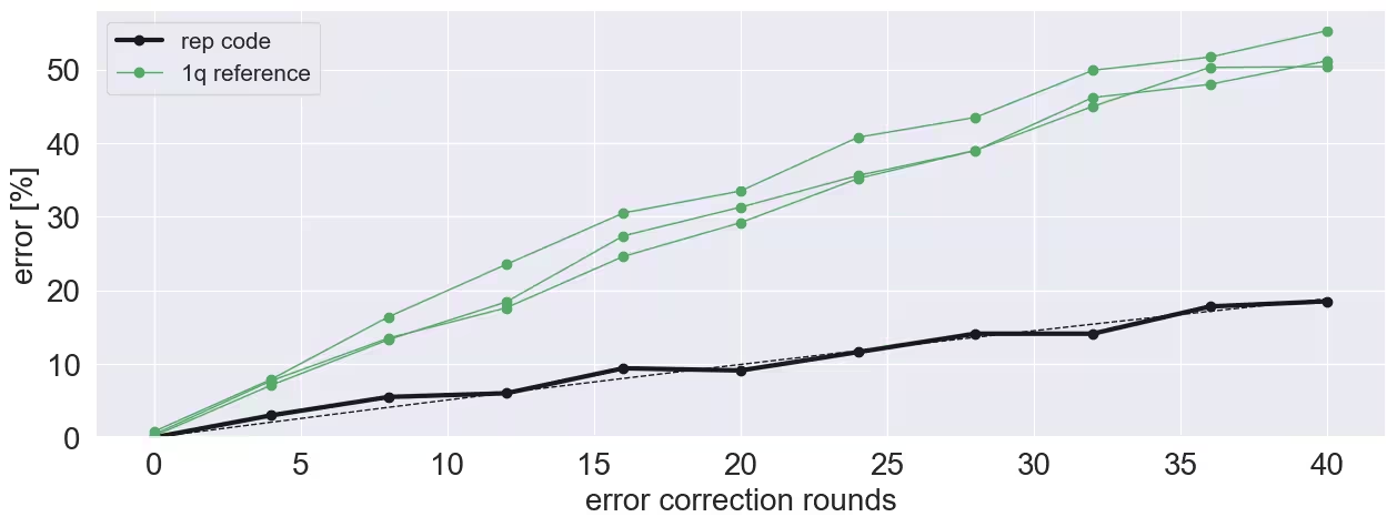
เราเห็นได้ชัดว่าอายุการใช้งานของสถานะ ดีขึ้น แม้เทียบกับคิวบิตทางกายภาพที่ดีที่สุด (ที่ไม่ได้เข้ารหัส) อย่างไรก็ตาม โปรดจำไว้ว่าการทดลองนี้แก้ไขความผิดพลาดเพียงประเภทเดียวเท่านั้น คือ bit-flip คุณสามารถปรับปรุงอายุการใช้งานของคิวบิตเชิงลอจิคัลได้หรือไม่? คุณอาจลองสำรวจการปรับดีเลย์ให้เหมาะสม การขยายขนาดของรหัส repetition ให้มากกว่า และอื่น ๆ
ขั้นตอนถัดไป
หากคุณสนใจงานนี้ คุณอาจสนใจเนื้อหาต่อไปนี้ด้วย:
-
คอร์ส Foundations of quantum error correction - เรียนรู้เพิ่มเติมเกี่ยวกับการแก้ไขความผิดพลาดควอนตัม
-
บทเรียน Low-overhead error detection with spacetime codes - เรียนรู้วิธีใช้ Pauli checks เพื่อตรวจจับความผิดพลาดและทำ post-select ตัวอย่าง