สูตร Multi-product เพื่อลดความผิดพลาด Trotter

ประมาณเวลาใช้งาน QPU: สี่นาทีบนโปรเซสเซอร์ Heron r2 (หมายเหตุ: นี่เป็นเพียงการประมาณเท่านั้น เวลาจริงอาจแตกต่างกัน)

พื้นหลัง

บทแนะนำนี้สาธิตวิธีใช้ Multi-Product Formula (MPF) เพื่อให้ได้ความผิดพลาด Trotter ที่ต่ำกว่าใน observable ของเรา เมื่อเทียบกับความผิดพลาดที่เกิดจาก Trotter Circuit ที่ลึกที่สุดที่เราจะรันจริง MPF ลดความผิดพลาด Trotter ของ Hamiltonian dynamics ผ่านการรวมเชิงเส้นแบบถ่วงน้ำหนักจากการรัน Circuit หลายครั้ง พิจารณาการหาค่าคาดหวังของ observable สำหรับสถานะควอนตัม $\rho(t)=e^{-i H t} \rho(0) e^{i H t}$ ที่มี Hamiltonian $H$ โดยสามารถใช้ Product Formulas (PFs) เพื่อประมาณ time-evolution $e^{-i H t}$ ด้วยวิธีดังนี้:

• เขียน Hamiltonian $H$ ในรูป $H=\sum_{a=1}^d F_a,$ โดยที่ $F_a$ เป็น Hermitian operators ซึ่งสามารถนำ unitary ที่สอดคล้องกันมาใช้งานบนอุปกรณ์ควอนตัมได้อย่างมีประสิทธิภาพ
• ประมาณค่าพจน์ $F_a$ ที่ไม่ commute ซึ่งกันและกัน

จากนั้น first-order PF (สูตร Lie-Trotter) คือ:

$S_1(t):=\prod_{a=1}^d e^{-i F_a t},$

ซึ่งมี error term เป็น quadratic $S_1(t)=e^{-i H t}+\mathcal{O}\left(t^{2}\right)$ นอกจากนี้ยังสามารถใช้ higher-order PFs (สูตร Lie-Trotter-Suzuki) ซึ่งมีการลู่เข้าที่เร็วกว่าและนิยามแบบ recursive ดังนี้:

$S_2(t):=\prod_{a=1}^d e^{-i F_a t/2}\prod_{a=1}^d e^{-i F_a t/2}$

$S_{2 \chi}(t):= S_{2 \chi -2}(s_{\chi}t)^2 S_{2 \chi -2}((1-4s_{\chi})t)S_{2 \chi -2}(s_{\chi}t)^2,$

โดยที่ $\chi$ คือลำดับของ symmetric PF และ $s_p = \left( 4 - 4^{1/(2p-1)} \right)^{-1}$ สำหรับ time-evolution ระยะยาว สามารถแบ่งช่วงเวลา $t$ ออกเป็น $k$ ช่วง เรียกว่า Trotter steps มีขนาด $t/k$ แต่ละช่วง และประมาณ time-evolution ในแต่ละช่วงด้วย product formula อันดับ $\chi$ คือ $S_{\chi}$ ดังนั้น PF อันดับ $\chi$ สำหรับ time-evolution operator ใน $k$ Trotter steps คือ:

$S_{\chi}^{k}(t) = \left[ S_{\chi} \left( \frac{t}{k} \right)\right]^k = e^{-i H t}+O\left(t \left( \frac{t}{k} \right)^{\chi} \right)$

โดย error term จะลดลงตามจำนวน Trotter steps $k$ และลำดับ $\chi$ ของ PF

สำหรับจำนวนเต็ม $k \geq 1$ และ product formula $S_{\chi}(t)$ สถานะที่ถูก time-evolve โดยประมาณ $\rho_k(t)$ สามารถหาได้จาก $\rho_0$ โดยการใช้ product formula $S_{\chi}\left(\frac{t}{k}\right)$ ซ้ำ $k$ ครั้ง

$$\rho_k(t)=S_{\chi}\left(\frac{t}{k}\right)^k \rho_0 S_{\chi}\left(\frac{t}{k}\right)^{-k}$$

$\rho_k(t)$ เป็นการประมาณของ $\rho(t)$ โดยมี Trotter approximation error คือ ||$\rho_k(t)-\rho(t) ||$ ถ้าพิจารณา linear combination ของ Trotter approximations ของ $\rho(t)$:

$$\mu(t) = \sum_{j}^{l} x_j \rho^{k_j}_{j}\left(\frac{t}{k_j}\right) + \text{some remaining Trotter error} \, ,$$

โดยที่ $x_j$ คือ weighting coefficients ของเรา $\rho^{k_j}_j$ คือ density matrix ที่สอดคล้องกับ pure state ที่ได้จากการ evolve สถานะเริ่มต้นด้วย product formula $S^{k_j}_{\chi}$ ที่ใช้ $k_j$ Trotter steps และ $j \in {1, ..., l}$ เป็น index ของจำนวน PFs ที่ประกอบขึ้นเป็น MPF ทุกพจน์ใน $\mu(t)$ ใช้ product formula $S_{\chi}(t)$ เดียวกันเป็นฐาน เป้าหมายคือการปรับปรุง ||$\rho_k(t)-\rho(t) \|$ โดยหา $\mu(t)$ ที่มี $\|\mu(t)-\rho(t)\|$ ต่ำกว่า

• $\mu(t)$ ไม่จำเป็นต้องเป็นสถานะทางกายภาพ เนื่องจาก $x_i$ ไม่จำเป็นต้องเป็นบวก เป้าหมายที่นี่คือการลดความผิดพลาดในค่าคาดหวังของ observables ไม่ใช่การหาตัวแทนทางกายภาพของ $\rho(t)$
• $k_j$ กำหนดทั้งความลึกของ Circuit และระดับของ Trotter approximation ค่า $k_j$ ที่เล็กกว่าจะให้ Circuit ที่สั้นกว่าซึ่งมีความผิดพลาดของ Circuit น้อยกว่า แต่จะเป็นการประมาณสถานะที่ต้องการได้แม่นยำน้อยกว่า

ประเด็นสำคัญคือ Trotter error ที่เหลืออยู่ที่ $\mu(t)$ ให้มานั้นเล็กกว่า Trotter error ที่จะได้จากการใช้ค่า $k_j$ ที่ใหญ่ที่สุดเพียงอย่างเดียว

สามารถมองประโยชน์ของสิ่งนี้ได้จากสองมุมมอง:

1. สำหรับงบประมาณ Trotter steps ที่กำหนดไว้ที่สามารถรันได้ สามารถได้ผลลัพธ์ที่มี Trotter error ต่ำกว่าโดยรวม
2. สำหรับจำนวน Trotter steps เป้าหมายที่มากเกินไปจะรัน สามารถใช้ MPF เพื่อหาชุด Circuit ความลึกต่ำกว่าที่จะรัน ซึ่งให้ Trotter error ที่ใกล้เคียงกัน

ข้อกำหนด

ก่อนเริ่มบทแนะนำนี้ ตรวจสอบว่าติดตั้งสิ่งต่อไปนี้แล้ว:

• Qiskit SDK v1.0 ขึ้นไป พร้อมรองรับ visualization
• Qiskit Runtime v0.22 ขึ้นไป (pip install qiskit-ibm-runtime)
• MPF Qiskit addons (pip install qiskit_addon_mpf)
• Qiskit addons utils (pip install qiskit_addon_utils)
• ไลบรารี Quimb (pip install quimb)
• ไลบรารี Qiskit Quimb (pip install qiskit-quimb)
• Numpy v0.21 สำหรับความเข้ากันได้ข้ามแพ็กเกจ (pip install numpy==0.21)

ส่วนที่ I ตัวอย่างขนาดเล็ก

สำรวจความเสถียรของ MPF

ไม่มีข้อจำกัดที่ชัดเจนเกี่ยวกับการเลือกจำนวน Trotter steps $k_j$ ที่ประกอบขึ้นเป็นสถานะ MPF $\mu(t)$ อย่างไรก็ตาม ต้องเลือกอย่างระมัดระวังเพื่อหลีกเลี่ยงความไม่เสถียรในค่าคาดหวังที่คำนวณจาก $\mu(t)$ กฎทั่วไปที่ดีคือตั้งค่า Trotter step ที่เล็กที่สุด $k_{\text{min}}$ ให้ $t/k_{\text{min}} \lt 1$ ถ้าต้องการเรียนรู้เพิ่มเติมเกี่ยวกับเรื่องนี้และวิธีเลือกค่า $k_j$ อื่น ๆ ดูได้ที่คู่มือ How to choose the Trotter steps for an MPF

ในตัวอย่างด้านล่างนี้ เราสำรวจความเสถียรของ MPF solution โดยคำนวณค่าคาดหวังของ magnetization สำหรับช่วงเวลาต่าง ๆ โดยใช้สถานะ time-evolved ที่แตกต่างกัน โดยเฉพาะอย่างยิ่ง เราเปรียบเทียบค่าคาดหวังที่คำนวณจาก time-evolution โดยประมาณแต่ละแบบที่ใช้ Trotter steps ที่สอดคล้องกัน และโมเดล MPF ต่าง ๆ (static และ dynamic coefficients) กับค่าที่แม่นยำของ observable ที่ถูก time-evolve ก่อนอื่น มากำหนดพารามิเตอร์สำหรับสูตร Trotter และช่วงเวลาที่ต้องการ

# Added by doQumentation — required packages for this notebook
!pip install -q matplotlib numpy qiskit qiskit-addon-mpf qiskit-addon-utils qiskit-aer qiskit-ibm-runtime rustworkx scipy

import numpy as np

mpf_trotter_steps = [1, 2, 4]
order = 2
symmetric = False

trotter_times = np.arange(0.5, 1.55, 0.1)
exact_evolution_times = np.arange(trotter_times[0], 1.55, 0.05)

สำหรับตัวอย่างนี้เราจะใช้สถานะ Neel เป็นสถานะเริ่มต้น $\vert \text{Neel} \rangle = \vert 0101...01 \rangle$ และโมเดล Heisenberg บนเส้นตรง 10 sites สำหรับ Hamiltonian ที่ควบคุม time-evolution

$$\hat{\mathcal{H}}_{Heis} = J \sum_{i=1}^{L-1} \left(X_i X_{(i+1)}+Y_i Y_{(i+1)}+ Z_i Z_{(i+1)} \right) \, ,$$

โดยที่ $J$ คือความแข็งแรงของการจับคู่สำหรับเส้นเชื่อมระหว่างเพื่อนบ้านที่ใกล้ที่สุด

from qiskit.transpiler import CouplingMap
from rustworkx.visualization import graphviz_draw
from qiskit_addon_utils.problem_generators import generate_xyz_hamiltonian
import numpy as np

L = 10

# Generate some coupling map to use for this example
coupling_map = CouplingMap.from_line(L, bidirectional=False)
graphviz_draw(coupling_map.graph, method="circo")

# Get a qubit operator describing the Heisenberg field model
hamiltonian = generate_xyz_hamiltonian(
    coupling_map,
    coupling_constants=(1.0, 1.0, 1.0),
    ext_magnetic_field=(0.0, 0.0, 0.0),
)

print(hamiltonian)

SparsePauliOp(['IIIIIIIXXI', 'IIIIIIIYYI', 'IIIIIIIZZI', 'IIIIIXXIII', 'IIIIIYYIII', 'IIIIIZZIII', 'IIIXXIIIII', 'IIIYYIIIII', 'IIIZZIIIII', 'IXXIIIIIII', 'IYYIIIIIII', 'IZZIIIIIII', 'IIIIIIIIXX', 'IIIIIIIIYY', 'IIIIIIIIZZ', 'IIIIIIXXII', 'IIIIIIYYII', 'IIIIIIZZII', 'IIIIXXIIII', 'IIIIYYIIII', 'IIIIZZIIII', 'IIXXIIIIII', 'IIYYIIIIII', 'IIZZIIIIII', 'XXIIIIIIII', 'YYIIIIIIII', 'ZZIIIIIIII'],
              coeffs=[1.+0.j, 1.+0.j, 1.+0.j, 1.+0.j, 1.+0.j, 1.+0.j, 1.+0.j, 1.+0.j, 1.+0.j,
 1.+0.j, 1.+0.j, 1.+0.j, 1.+0.j, 1.+0.j, 1.+0.j, 1.+0.j, 1.+0.j, 1.+0.j,
 1.+0.j, 1.+0.j, 1.+0.j, 1.+0.j, 1.+0.j, 1.+0.j, 1.+0.j, 1.+0.j, 1.+0.j])

Observable ที่เราจะวัดคือ magnetization ของคู่ Qubits ตรงกลาง chain

from qiskit.quantum_info import SparsePauliOp

observable = SparsePauliOp.from_sparse_list(
    [("ZZ", (L // 2 - 1, L // 2), 1.0)], num_qubits=L
)
print(observable)

SparsePauliOp(['IIIIZZIIII'],
              coeffs=[1.+0.j])

เรานิยาม transpiler pass เพื่อรวบรวม XX และ YY rotations ใน Circuit เป็น Gate XX+YY ตัวเดียว ซึ่งจะช่วยให้เราใช้ประโยชน์จากคุณสมบัติการอนุรักษ์ spin ของ TeNPy ระหว่างการคำนวณ MPO ซึ่งเพิ่มความเร็วในการคำนวณอย่างมาก

from qiskit.circuit.library import XXPlusYYGate
from qiskit.transpiler import PassManager
from qiskit.transpiler.passes.optimization.collect_and_collapse import (
    CollectAndCollapse,
    collect_using_filter_function,
    collapse_to_operation,
)
from functools import partial

def filter_function(node):
    return node.op.name in {"rxx", "ryy"}

collect_function = partial(
    collect_using_filter_function,
    filter_function=filter_function,
    split_blocks=True,
    min_block_size=1,
)

def collapse_to_xx_plus_yy(block):
    param = 0.0
    for node in block.data:
        param += node.operation.params[0]
    return XXPlusYYGate(param)

collapse_function = partial(
    collapse_to_operation,
    collapse_function=collapse_to_xx_plus_yy,
)

pm = PassManager()
pm.append(CollectAndCollapse(collect_function, collapse_function))

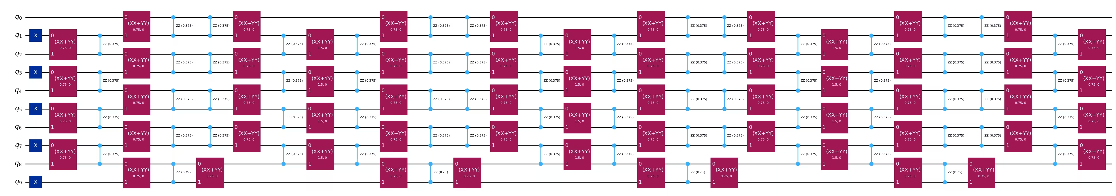
จากนั้นเราสร้าง Circuit ที่ใช้งาน Trotter time-evolution โดยประมาณ

from qiskit.synthesis import SuzukiTrotter
from qiskit_addon_utils.problem_generators import (
    generate_time_evolution_circuit,
)
from qiskit import QuantumCircuit

# Initial Neel state preparation
initial_state_circ = QuantumCircuit(L)
initial_state_circ.x([i for i in range(L) if i % 2 != 0])

all_circs = []
for total_time in trotter_times:
    mpf_trotter_circs = [
        generate_time_evolution_circuit(
            hamiltonian,
            time=total_time,
            synthesis=SuzukiTrotter(reps=num_steps, order=order),
        )
        for num_steps in mpf_trotter_steps
    ]

    mpf_trotter_circs = pm.run(
        mpf_trotter_circs
    )  # Collect XX and YY into XX + YY

    mpf_circuits = [
        initial_state_circ.compose(circuit) for circuit in mpf_trotter_circs
    ]
    all_circs.append(mpf_circuits)

mpf_circuits[-1].draw("mpl", fold=-1)

ต่อไป เราคำนวณค่าคาดหวัง time-evolved จาก Trotter Circuit

from copy import deepcopy
from qiskit_aer import AerSimulator
from qiskit_ibm_runtime import EstimatorV2 as Estimator
from qiskit.transpiler.preset_passmanagers import generate_preset_pass_manager

aer_sim = AerSimulator()
estimator = Estimator(mode=aer_sim)

mpf_expvals_all_times, mpf_stds_all_times = [], []
for t, mpf_circuits in zip(trotter_times, all_circs):
    mpf_expvals = []
    circuits = [deepcopy(circuit) for circuit in mpf_circuits]
    pm_sim = generate_preset_pass_manager(
        backend=aer_sim, optimization_level=3
    )
    isa_circuits = pm_sim.run(circuits)
    result = estimator.run(
        [(circuit, observable) for circuit in isa_circuits], precision=0.005
    ).result()
    mpf_expvals = [res.data.evs for res in result]
    mpf_stds = [res.data.stds for res in result]
    mpf_expvals_all_times.append(mpf_expvals)
    mpf_stds_all_times.append(mpf_stds)

เรายังคำนวณค่าคาดหวังที่แม่นยำสำหรับการเปรียบเทียบด้วย

from scipy.linalg import expm
from qiskit.quantum_info import Statevector

exact_expvals = []
for t in exact_evolution_times:
    # Exact expectation values
    exp_H = expm(-1j * t * hamiltonian.to_matrix())
    initial_state = Statevector(initial_state_circ).data
    time_evolved_state = exp_H @ initial_state

    exact_obs = (
        time_evolved_state.conj()
        @ observable.to_matrix()
        @ time_evolved_state
    ).real
    exact_expvals.append(exact_obs)

Static MPF coefficients

Static MPF คือ MPF ที่ค่า $x_j$ ไม่ขึ้นกับเวลา evolution $t$ ลองพิจารณา PF อันดับ $\chi = 1$ ที่มี $k_j$ Trotter steps สามารถเขียนได้เป็น:

$S_1^{k_j}\left( \frac{t}{k_j} \right)=e^{-i H t}+ \sum_{n=1}^{\infty} A_n \frac{t^{n+1}}{k_j^n}$

โดยที่ $A_n$ คือเมทริกซ์ที่ขึ้นกับ commutators ของพจน์ $F_a$ ในการ decompose ของ Hamiltonian สิ่งสำคัญคือต้องสังเกตว่า $A_n$ เองนั้นเป็นอิสระจากเวลาและจำนวน Trotter steps $k_j$ ดังนั้นจึงเป็นไปได้ที่จะตัด lower-order error terms ที่มีส่วนร่วมใน $\mu(t)$ ด้วยการเลือก weights $x_j$ ของ linear combination อย่างระมัดระวัง เพื่อตัด Trotter error สำหรับ $l-1$ พจน์แรก (พจน์เหล่านี้จะมีส่วนร่วมมากที่สุดเนื่องจากสอดคล้องกับจำนวน Trotter steps ที่น้อยกว่า) ในนิพจน์ของ $\mu(t)$ coefficients $x_j$ ต้องเป็นไปตามสมการดังนี้:

$\sum_{j=1}^l x_j = 1$ $\sum_{j=1}^{l-1} \frac{x_j}{k_j^{n}} = 0$

โดย $n=0, ... l-2$ สมการแรกรับประกันว่าไม่มี bias ในสถานะ $\mu(t)$ ที่สร้างขึ้น ในขณะที่สมการที่สองรับประกันการตัด Trotter errors สำหรับ PF อันดับสูงกว่า สมการที่สองกลายเป็น $\sum_{j=1}^{l-1} \frac{x_j}{k_j^{\eta}} = 0$ โดยที่ $\eta = \chi + 2n$ สำหรับ symmetric PFs และ $\eta = \chi + n$ สำหรับกรณีอื่น ๆ โดย $n=0, ..., l-2$ ความผิดพลาดที่ได้ (อ้างอิง [1],[2]) คือ

$\epsilon = \mathcal{O} \left( \frac{t^{l+1}}{k_1^l} \right).$

การหา static MPF coefficients สำหรับชุดค่า $k_j$ ที่กำหนดนั้นเทียบเท่ากับการแก้ระบบสมการเชิงเส้นที่นิยามโดยสมการทั้งสองข้างต้นสำหรับตัวแปร $x_j$: $Ax=b$ โดยที่ $x$ คือ coefficients ที่เราต้องการ $A$ คือเมทริกซ์ที่ขึ้นกับ $k_j$ และประเภทของ PF ที่ใช้ ($S$) และ $b$ คือเวกเตอร์ของ constraints โดยเฉพาะอย่างยิ่ง:

$A_{0,j} = 1$ $A_{i>0,j} = k_{j}^{-(\chi + s(i-1))}$ $b_0 = 1$ $b_{i>0} = 0$

โดยที่ $\chi$ คือ order, $s$ คือ $2$ ถ้า symmetric เป็น True และ $1$ สำหรับกรณีอื่น ๆ $k_{j}$ คือ trotter_steps และ $x$ คือตัวแปรที่ต้องการแก้ index $i$ และ $j$ เริ่มที่ $0$ เราสามารถแสดงในรูปเมทริกซ์ได้เช่นกัน:

$$A = \begin{bmatrix} A_{0,0} & A_{0,1} & A_{0,2} & ... \\ A_{1,0} & A_{1,1} & A_{1,2} & ... \\ A_{2,0} & A_{2,1} & A_{2,2} & ... \\ ... & ... & ... & ... \end{bmatrix} = \begin{bmatrix} 1 & 1 & 1 & ... \\ k_{0}^{-(\chi + s(1-1))} & k_{1}^{-(\chi + s(1-1))} & k_{2}^{-(\chi + s(1-1))} & ... \\ k_{0}^{-(\chi + s(2-1))} & k_{1}^{-(\chi + s(2-1))} & k_{2}^{-(\chi + s(2-1))} & ... \\ ... & ... & ... & ... \end{bmatrix}$$

และ

$$b = \begin{bmatrix} b_{0} \\ b_{1} \\ b_{2} \\ ... \end{bmatrix} = \begin{bmatrix} 1 \\ 0 \\ 0 \\ ... \end{bmatrix}$$

สำหรับรายละเอียดเพิ่มเติม ดูเอกสารของ Linear System of Equations (LSE)

เราสามารถหาคำตอบสำหรับ $x$ ได้เชิงวิเคราะห์เป็น $x = A^{-1}b$ ดูตัวอย่างในอ้างอิง [1] หรือ [2] อย่างไรก็ตาม คำตอบที่แม่นยำนี้อาจ "ill-conditioned" ส่งผลให้ L1-norm ของ coefficients $x$ ของเราใหญ่มาก ซึ่งอาจทำให้ MPF มีประสิทธิภาพต่ำ แต่สามารถใช้คำตอบโดยประมาณที่ minimize L1-norm ของ $x$ แทน เพื่อพยายาม optimize พฤติกรรม MPF

ตั้งค่า LSE

เมื่อเลือกค่า $k_j$ แล้ว ขั้นแรกต้องสร้าง LSE ก่อน คือ $Ax=b$ ตามที่อธิบายข้างต้น เมทริกซ์ $A$ ขึ้นกับไม่เพียงแค่ $k_j$ แต่ยังขึ้นกับตัวเลือก PF ของเรา โดยเฉพาะ order ของมัน นอกจากนี้อาจต้องพิจารณาว่า PF เป็น symmetric หรือไม่ (ดู [1]) โดยตั้งค่า symmetric=True/False อย่างไรก็ตามนี่ไม่ใช่ข้อบังคับ ตามที่อ้างอิง [2] แสดงให้เห็น

from qiskit_addon_mpf.static import setup_static_lse

lse = setup_static_lse(mpf_trotter_steps, order=order, symmetric=symmetric)

มาดูค่าที่เลือกข้างต้นเพื่อสร้างเมทริกซ์ $A$ และเวกเตอร์ $b$ ด้วยค่า $j=0,1, 2$ Trotter steps $k_j = [1, 2, 4]$, order $\chi = 2$ และการเลือก non-symmetric Trotter steps ($s=1$) elements ของเมทริกซ์ $A$ ในแถวที่ต่ำกว่าแถวแรกถูกกำหนดโดยนิพจน์ $A_{i>0,j} = k_{j}^{-(2 + 1(i-1))}$ โดยเฉพาะอย่างยิ่ง:

$A_{0,0} = A_{0,1} = A_{0,2} = 1$ $A_{1,j} = k_{j}^{-1} \rightarrow A_{1,0} = \frac{1}{1^2}, \;, A_{1,1} = \frac{1}{2^2}, \;, A_{1,2} = \frac{1}{4^2}$ $A_{2,j} = k_{j}^{-2} \rightarrow A_{2,0} = \frac{1}{1^3}, \;, A_{2,1} = \frac{1}{2^3}, \;, A_{2,2} = \frac{1}{4^3}$

หรือในรูปเมทริกซ์:

$$A = \begin{bmatrix} 1 & 1 & 1\\ 1 & \frac{1}{2^2} & \frac{1}{4^2} \\ 1 & \frac{1}{2^3} & \frac{1}{4^3} \\ \end{bmatrix}$$

สามารถดูได้โดยตรวจสอบ object lse:

lse.A

array([[1.      , 1.      , 1.      ],
       [1.      , 0.25    , 0.0625  ],
       [1.      , 0.125   , 0.015625]])

ส่วนเวกเตอร์ของ constraints $b$ มี elements ดังนี้: $b_{0} = 1$ $b_1 = b_2 = 0$

ดังนั้น

$$b = \begin{bmatrix} 1 \\ 0 \\ 0 \end{bmatrix}$$

และในทำนองเดียวกันใน lse:

lse.b

array([1., 0., 0.])

Object lse มีเมธอดสำหรับหา static coefficients $x_j$ ที่เป็นไปตามระบบสมการ

mpf_coeffs = lse.solve()
print(
    f"The static coefficients associated with the ansatze are: {mpf_coeffs}"
)

The static coefficients associated with the ansatze are: [ 0.04761905 -0.57142857  1.52380952]

หาค่า $x$ ที่เหมาะสมโดยใช้ exact model

นอกจากการคำนวณ $x=A^{-1}b$ แล้ว ยังสามารถใช้ setup_exact_model เพื่อสร้าง instance ของ cvxpy.Problem ที่ใช้ LSE เป็น constraints และ optimal solution ของมันจะให้ค่า $x$

ในส่วนถัดไปจะเห็นได้ชัดว่าทำไม interface นี้จึงมีอยู่

from qiskit_addon_mpf.costs import setup_exact_problem

model_exact, coeffs_exact = setup_exact_problem(lse)
model_exact.solve()
print(coeffs_exact.value)

[ 0.04761905 -0.57142857  1.52380952]

เป็นตัวบ่งชี้ว่า MPF ที่สร้างด้วย coefficients เหล่านี้จะให้ผลลัพธ์ที่ดีหรือไม่ เราสามารถใช้ L1-norm (ดูอ้างอิง [1] ด้วย)

print(
    "L1 norm of the exact coefficients:",
    np.linalg.norm(coeffs_exact.value, ord=1),
)  # ord specifies the norm. ord=1 is for L1

L1 norm of the exact coefficients: 2.1428571428556378

หาค่า $x$ ที่เหมาะสมโดยใช้ approximate model

อาจเกิดขึ้นได้ที่ L1 norm สำหรับชุดค่า $k_j$ ที่เลือกถูกพิจารณาว่าสูงเกินไป หากเป็นเช่นนั้นและไม่สามารถเลือกชุดค่า $k_j$ ที่ต่างออกไปได้ สามารถใช้คำตอบโดยประมาณของ LSE แทนคำตอบที่แม่นยำ

ทำได้โดยใช้ setup_approximate_model เพื่อสร้าง instance ของ cvxpy.Problem ที่แตกต่างกัน ซึ่งจำกัด L1-norm ไว้ที่ threshold ที่เลือก โดย minimize ความแตกต่างของ $Ax$ และ $b$

from qiskit_addon_mpf.costs import setup_sum_of_squares_problem

model_approx, coeffs_approx = setup_sum_of_squares_problem(
    lse, max_l1_norm=1.5
)
model_approx.solve()
print(coeffs_approx.value)
print(
    "L1 norm of the approximate coefficients:",
    np.linalg.norm(coeffs_approx.value, ord=1),
)

[-1.10294118e-03 -2.48897059e-01  1.25000000e+00]
L1 norm of the approximate coefficients: 1.5

สังเกตว่ามีอิสระสมบูรณ์ในการแก้ปัญหา optimization นี้ ซึ่งหมายความว่าสามารถเปลี่ยน optimization solver, convergence thresholds ของมัน และอื่น ๆ ได้ ดูคู่มือที่เกี่ยวข้องเรื่อง How to use the approximate model.

Dynamic MPF coefficients

ในส่วนก่อนหน้า เราแนะนำ static MPF ที่ปรับปรุงจาก Trotter approximation มาตรฐาน อย่างไรก็ตาม static version นี้ไม่จำเป็นต้อง minimize approximation error เสมอไป โดยเฉพาะอย่างยิ่ง static MPF ที่แทนด้วย $\mu^S(t)$ ไม่ใช่ optimal projection ของ $\rho(t)$ ลงบน subspace ที่สร้างขึ้นโดยสถานะ product-formula $\{\rho_{k_i}(t)\}_{i=1}^r$

เพื่อแก้ไขปัญหานี้ เราพิจารณา dynamic MPF (แนะนำในอ้างอิง [2] และแสดงให้เห็นเชิงทดลองในอ้างอิง [3]) ที่ minimize approximation error ใน Frobenius norm อย่างแท้จริง โดยเป็นทางการ เราเน้นที่การ minimize

$$\|\rho(t) - \mu^D(t)\|_F^2 \;=\; \mathrm{Tr}\bigl[ \left( \rho(t) - \mu^D(t)\right)^2 \bigr],$$

สำหรับ coefficients $x_i(t)$ บางตัวในแต่ละเวลา $t$ optimal projector ใน Frobenius norm คือ $\mu^D(t) \;=\; \sum_{i=1}^r x_i(t)\,\rho_{k_i}(t)$ และเราเรียก $\mu^D(t)$ ว่า dynamic MPF เมื่อแทนค่านิยามข้างต้น:

$$\|\rho(t) - \mu^D(t)\|_F^2 \;=\; \\ = \mathrm{Tr}\bigl[ \left( \rho(t) - \mu^D(t)\right)^2 \bigr] \;=\; \\ = \mathrm{Tr}\bigl[ \left( \rho(t) - \sum_{i=1}^r x_i(t)\,\rho_{k_i}(t) \right) \left( \rho(t) - \sum_{j=1}^r x_j(t)\,\rho_{k_j}(t) \right) \bigr] \;=\; \\ = 1 \;+\; \sum_{i,j=1}^r M_{i,j}(t)\,x_i(t)\,x_j(t) \;-\; 2 \sum_{i=1}^r L_i^{\mathrm{exact}}(t)\,x_i(t),$$

โดยที่ $M_{i,j}(t)$ คือ Gram matrix นิยามโดย

$$M_{i,j}(t) \;=\; \mathrm{Tr}\bigl[\rho_{k_i}(t)\,\rho_{k_j}(t)\bigr] \;=\; \bigl|\langle \psi_{\mathrm{in}} \!\mid S\bigl(t/k_i\bigr)^{-k_i}\,S\bigl(t/k_j\bigr)^{k_j} \!\mid \psi_{\mathrm{in}} \rangle \bigr|^2.$$

และ

$$L_i^{\mathrm{exact}}(t) = \mathrm{Tr}[\rho(t)\,\rho_{k_i}(t)]$$

แทน overlap ระหว่างสถานะที่แม่นยำ $\rho(t)$ และ product-formula approximation $\rho_{k_i}(t)$ แต่ละตัว ในสถานการณ์จริง overlaps เหล่านี้อาจวัดได้เพียงโดยประมาณเนื่องจาก noise หรือการเข้าถึง $\rho(t)$ บางส่วน

ที่นี่ $\lvert\psi_{\mathrm{in}}\rangle$ คือสถานะเริ่มต้น และ $S(\cdot)$ คือการดำเนินการที่ใช้ใน product formula การเลือก coefficients $x_i(t)$ ที่ minimize นิพจน์นี้ (และจัดการกับข้อมูล overlap โดยประมาณเมื่อ $\rho(t)$ ไม่เป็นที่ทราบอย่างสมบูรณ์) ทำให้ได้ dynamic approximation ที่ "ดีที่สุด" (ในแง่ Frobenius-norm) ของ $\rho(t)$ ภายใน MPF subspace ปริมาณ $L_i(t)$ และ $M_{i,j}(t)$ สามารถคำนวณได้อย่างมีประสิทธิภาพโดยใช้ tensor network methods [3] MPF Qiskit addon มี "backends" หลายตัวสำหรับการคำนวณนี้ ตัวอย่างด้านล่างแสดงวิธีที่ยืดหยุ่นที่สุด และเอกสาร TeNPy layer-based backend ยังอธิบายรายละเอียดอย่างครบถ้วน เพื่อใช้วิธีนี้ เริ่มจาก Circuit ที่ใช้งาน time-evolution ที่ต้องการ และสร้าง models ที่แทนการดำเนินการเหล่านี้จาก layers ของ Circuit ที่สอดคล้องกัน สุดท้าย object Evolver จะถูกสร้างขึ้นซึ่งสามารถใช้สร้างปริมาณ time-evolved $M_{i,j}(t)$ และ $L_i(t)$ ได้ เริ่มต้นโดยการสร้าง object Evolver ที่สอดคล้องกับ approximate time-evolution (ApproxEvolverFactory) ที่ใช้งานโดย Circuit โดยเฉพาะอย่างยิ่ง ให้ใส่ใจตัวแปร order เป็นพิเศษเพื่อให้ตรงกัน สังเกตว่าในการสร้าง Circuit ที่สอดคล้องกับ approximate time-evolution เราใช้ค่า placeholder สำหรับ time = 1.0 และจำนวน Trotter steps (reps=1) Circuit ที่ประมาณค่าที่ถูกต้องจะถูกสร้างโดย dynamic problem solver ใน setup_dynamic_lse

from qiskit_addon_utils.slicing import slice_by_depth
from qiskit_addon_mpf.backends.tenpy_layers import LayerModel
from qiskit_addon_mpf.backends.tenpy_layers import LayerwiseEvolver
from functools import partial

# Create approximate time-evolution circuits
single_2nd_order_circ = generate_time_evolution_circuit(
    hamiltonian, time=1.0, synthesis=SuzukiTrotter(reps=1, order=order)
)
single_2nd_order_circ = pm.run(single_2nd_order_circ)  # collect XX and YY

# Find layers in the circuit
layers = slice_by_depth(single_2nd_order_circ, max_slice_depth=1)

# Create tensor network models
models = [
    LayerModel.from_quantum_circuit(layer, conserve="Sz") for layer in layers
]

# Create the time-evolution object
approx_factory = partial(
    LayerwiseEvolver,
    layers=models,
    options={
        "preserve_norm": False,
        "trunc_params": {
            "chi_max": 64,
            "svd_min": 1e-8,
            "trunc_cut": None,
        },
        "max_delta_t": 2,
    },
)

คำเตือน

ตัวเลือกของ LayerwiseEvolver ที่กำหนดรายละเอียดของ tensor network simulation ต้องถูกเลือกอย่างระมัดระวังเพื่อหลีกเลี่ยงการตั้งค่าปัญหา optimization ที่ไม่ถูกต้อง

จากนั้นเราตั้งค่า exact evolver (เช่น ExactEvolverFactory) ซึ่งคืน object Evolver ที่คำนวณ time-evolution ที่แท้จริงหรือ "reference" ในทางปฏิบัติ เราจะประมาณ exact evolution โดยใช้สูตร Suzuki–Trotter อันดับสูงกว่าหรือวิธีที่เชื่อถือได้อื่น ๆ ที่มี time step เล็ก ด้านล่างนี้ เราประมาณสถานะ exact time-evolved ด้วยสูตร Suzuki-Trotter อันดับสี่โดยใช้ time step เล็ก dt=0.1 ซึ่งหมายความว่าจำนวน Trotter steps ที่ใช้ในเวลา $t$ คือ $k=t/dt$ เรายังระบุตัวเลือก truncation เฉพาะของ TeNPy เพื่อจำกัด maximum bond dimension ของ underlying tensor network รวมถึง singular values ต่ำสุดของ split tensor network bonds พารามิเตอร์เหล่านี้สามารถส่งผลต่อความแม่นยำของค่าคาดหวังที่คำนวณด้วย dynamic MPF coefficients ดังนั้นสิ่งสำคัญคือต้องสำรวจค่าต่าง ๆ เพื่อหาสมดุลที่เหมาะสมระหว่างเวลาคำนวณและความแม่นยำ สังเกตว่าการคำนวณ MPF coefficients ไม่ได้อาศัยค่าคาดหวังของ PF ที่ได้จากการรันบน hardware ดังนั้นจึงสามารถปรับแต่งใน post-processing ได้

single_4th_order_circ = generate_time_evolution_circuit(
    hamiltonian, time=1.0, synthesis=SuzukiTrotter(reps=1, order=4)
)
single_4th_order_circ = pm.run(single_4th_order_circ)
exact_model_layers = [
    LayerModel.from_quantum_circuit(layer, conserve="Sz")
    for layer in slice_by_depth(single_4th_order_circ, max_slice_depth=1)
]

exact_factory = partial(
    LayerwiseEvolver,
    layers=exact_model_layers,
    dt=0.1,
    options={
        "preserve_norm": False,
        "trunc_params": {
            "chi_max": 64,
            "svd_min": 1e-8,
            "trunc_cut": None,
        },
        "max_delta_t": 2,
    },
)

ต่อไป สร้างสถานะเริ่มต้นของระบบในรูปแบบที่เข้ากันได้กับ TeNPy (เช่น MPS_neel_state=$\vert 0101...01 \rangle$) ซึ่งตั้งค่า many-body wavefunction ที่จะ evolve ตามเวลา $\lvert\psi_{\mathrm{in}}\rangle$ ในรูป tensor

from qiskit_addon_mpf.backends.tenpy_tebd import MPOState
from qiskit_addon_mpf.backends.tenpy_tebd import MPS_neel_state

def identity_factory():
    return MPOState.initialize_from_lattice(models[0].lat, conserve=True)

mps_initial_state = MPS_neel_state(models[0].lat)

สำหรับแต่ละ time step $t$ เราตั้งค่า dynamic linear system of equations ด้วยเมธอด setup_dynamic_lse object ที่สอดคล้องกันมีข้อมูลเกี่ยวกับ dynamic MPF problem: lse.A ให้ Gram matrix $M$ ส่วน lse.b ให้ overlap $L$ จากนั้นสามารถแก้ LSE (เมื่อไม่ ill-defined) เพื่อหา dynamic coefficients โดยใช้ setup_frobenius_problem สิ่งสำคัญคือต้องสังเกตความแตกต่างกับ static coefficients ซึ่งขึ้นกับเพียงรายละเอียดของ product formula ที่ใช้และเป็นอิสระจากรายละเอียดของ time-evolution (Hamiltonian และสถานะเริ่มต้น)

from qiskit_addon_mpf.dynamic import setup_dynamic_lse
from qiskit_addon_mpf.costs import setup_frobenius_problem

mpf_dynamic_coeffs_list = []
for t in trotter_times:
    print(f"Computing dynamic coefficients for time={t}")
    lse = setup_dynamic_lse(
        mpf_trotter_steps,
        t,
        identity_factory,
        exact_factory,
        approx_factory,
        mps_initial_state,
    )
    problem, coeffs = setup_frobenius_problem(lse)
    try:
        problem.solve()
        mpf_dynamic_coeffs_list.append(coeffs.value)
    except Exception as error:
        mpf_dynamic_coeffs_list.append(np.zeros(len(mpf_trotter_steps)))
        print(error, "Calculation Failed for time", t)
    print("")

Computing dynamic coefficients for time=0.5

Computing dynamic coefficients for time=0.6

Computing dynamic coefficients for time=0.7

Computing dynamic coefficients for time=0.7999999999999999

Computing dynamic coefficients for time=0.8999999999999999

Computing dynamic coefficients for time=0.9999999999999999

Computing dynamic coefficients for time=1.0999999999999999

Computing dynamic coefficients for time=1.1999999999999997

Computing dynamic coefficients for time=1.2999999999999998

Computing dynamic coefficients for time=1.4

Computing dynamic coefficients for time=1.4999999999999998

สุดท้าย แสดงกราฟค่าคาดหวังเหล่านี้ตลอดช่วงเวลา evolution

import matplotlib.pyplot as plt

sym = {1: "^", 2: "s", 4: "p"}
# Get expectation values at all times for each Trotter step
for k, step in enumerate(mpf_trotter_steps):
    trotter_curve, trotter_curve_error = [], []
    for trotter_expvals, trotter_stds in zip(
        mpf_expvals_all_times, mpf_stds_all_times
    ):
        trotter_curve.append(trotter_expvals[k])
        trotter_curve_error.append(trotter_stds[k])

    plt.errorbar(
        trotter_times,
        trotter_curve,
        yerr=trotter_curve_error,
        alpha=0.5,
        markersize=4,
        marker=sym[step],
        color="grey",
        label=f"{mpf_trotter_steps[k]} Trotter steps",
    )  # , , )

# Get expectation values at all times for the static MPF with exact coeffs
exact_mpf_curve, exact_mpf_curve_error = [], []
for trotter_expvals, trotter_stds in zip(
    mpf_expvals_all_times, mpf_stds_all_times
):
    mpf_std = np.sqrt(
        sum(
            [
                (coeff**2) * (std**2)
                for coeff, std in zip(coeffs_exact.value, trotter_stds)
            ]
        )
    )
    exact_mpf_curve_error.append(mpf_std)
    exact_mpf_curve.append(trotter_expvals @ coeffs_exact.value)

plt.errorbar(
    trotter_times,
    exact_mpf_curve,
    yerr=exact_mpf_curve_error,
    markersize=4,
    marker="o",
    label="Static MPF - Exact",
    color="purple",
)

# Get expectation values at all times for the static MPF with approximate
approx_mpf_curve, approx_mpf_curve_error = [], []
for trotter_expvals, trotter_stds in zip(
    mpf_expvals_all_times, mpf_stds_all_times
):
    mpf_std = np.sqrt(
        sum(
            [
                (coeff**2) * (std**2)
                for coeff, std in zip(coeffs_approx.value, trotter_stds)
            ]
        )
    )
    approx_mpf_curve_error.append(mpf_std)
    approx_mpf_curve.append(trotter_expvals @ coeffs_approx.value)

plt.errorbar(
    trotter_times,
    approx_mpf_curve,
    yerr=approx_mpf_curve_error,
    markersize=4,
    marker="o",
    color="orange",
    label="Static MPF - Approximate",
)

# # Get expectation values at all times for the dynamic MPF
dynamic_mpf_curve, dynamic_mpf_curve_error = [], []
for trotter_expvals, trotter_stds, dynamic_coeffs in zip(
    mpf_expvals_all_times, mpf_stds_all_times, mpf_dynamic_coeffs_list
):
    mpf_std = np.sqrt(
        sum(
            [
                (coeff**2) * (std**2)
                for coeff, std in zip(dynamic_coeffs, trotter_stds)
            ]
        )
    )
    dynamic_mpf_curve_error.append(mpf_std)
    dynamic_mpf_curve.append(trotter_expvals @ dynamic_coeffs)

plt.errorbar(
    trotter_times,
    dynamic_mpf_curve,
    yerr=dynamic_mpf_curve_error,
    markersize=4,
    marker="o",
    color="pink",
    label="Dynamic MPF",
)

plt.plot(
    exact_evolution_times,
    exact_expvals,
    lw=3,
    color="red",
    label="Exact time-evolution",
)

plt.title(
    f"Expectation values for (ZZ,{(L//2-1, L//2)}) as a function of time"
)
plt.xlabel("Time")
plt.ylabel("Expectation Value")
plt.legend()
plt.grid()

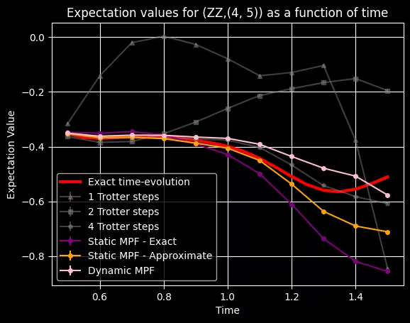
ในกรณีเช่นตัวอย่างข้างต้น ที่ PF ของ $k=1$ ทำงานได้ไม่ดีในทุกเวลา คุณภาพของผลลัพธ์ dynamic MPF ก็ได้รับผลกระทบอย่างมากเช่นกัน ในสถานการณ์เช่นนี้ มีประโยชน์ที่จะสำรวจความเป็นไปได้ในการใช้ PF แต่ละตัวที่มีจำนวน Trotter steps สูงกว่าเพื่อปรับปรุงคุณภาพโดยรวม ในการจำลองเหล่านี้ เราเห็นอันตรกิริยาของ error ประเภทต่าง ๆ ได้แก่ error จาก finite sampling และ Trotter error จาก product formulas MPF ช่วยลด Trotter error ที่เกิดจาก product formulas แต่มี sampling error สูงกว่าเมื่อเทียบกับ product formulas ซึ่งอาจเป็นประโยชน์ เนื่องจาก product formulas สามารถลด sampling error ได้ด้วยการเพิ่ม sampling แต่ systematic error ที่เกิดจาก Trotter approximation ยังคงอยู่

พฤติกรรมที่น่าสนใจอีกอย่างหนึ่งที่เราสังเกตได้จากกราฟคือค่าคาดหวังของ PF สำหรับ $k=1$ เริ่มมีพฤติกรรมผิดปกติ (นอกเหนือจากที่ไม่เป็นการประมาณที่ดีสำหรับค่าที่แม่นยำ) ในช่วงเวลาที่ $t/k > 1$ ตามที่อธิบายในคู่มือ เรื่องวิธีเลือกจำนวน Trotter steps

ขั้นตอนที่ 1: แมปข้อมูลนำเข้าแบบคลาสสิกไปยังปัญหาควอนตัม

มาพิจารณาเวลาเดี่ยว $t=1.0$ และคำนวณค่าความคาดหวังของการแมกเนไทเซชันด้วยวิธีต่างๆ โดยใช้ QPU หนึ่งตัว การเลือก $t$ นี้ทำขึ้นเพื่อให้ความแตกต่างระหว่างวิธีต่างๆ มีค่าสูงสุด และสังเกตประสิทธิภาพสัมพัทธ์ของแต่ละวิธี เพื่อกำหนดช่วงเวลาที่ dynamic MPF รับประกันว่าจะให้ค่าออบเซิร์ฟเวเบิลที่มีความผิดพลาดน้อยกว่าสูตร Trotter แต่ละสูตรภายใน multi-product เราสามารถใช้ "MPF test" ได้ — ดูสมการ (17) และข้อความโดยรอบใน [3]

ตั้งค่า Circuit ของ Trotter

ณ จุดนี้ เราได้ค้นพบค่าสัมประสิทธิ์การขยาย $x$ แล้ว และสิ่งที่เหลืออยู่คือการสร้าง Circuit ควอนตัมแบบ Trotterized โมดูล qiskit_addon_utils.problem_generators มาช่วยอีกครั้งพร้อมฟังก์ชันที่มีประโยชน์สำหรับทำสิ่งนี้:

from qiskit.synthesis import SuzukiTrotter
from qiskit_addon_utils.problem_generators import (
    generate_time_evolution_circuit,
)
from qiskit import QuantumCircuit

total_time = 1.0
mpf_circuits = []
for k in mpf_trotter_steps:
    # Initial Neel state preparation
    circuit = QuantumCircuit(L)
    circuit.x([i for i in range(L) if i % 2 != 0])

    trotter_circ = generate_time_evolution_circuit(
        hamiltonian,
        synthesis=SuzukiTrotter(order=order, reps=k),
        time=total_time,
    )

    circuit.compose(trotter_circ, inplace=True)

    mpf_circuits.append(pm.run(circuit))

mpf_circuits[-1].draw("mpl", fold=-1, scale=0.4)

ขั้นตอนที่ 2: ปรับแต่งปัญหาสำหรับการรันบนฮาร์ดแวร์ควอนตัม

กลับมาที่การคำนวณค่าความคาดหวังสำหรับจุดเวลาเดียว เราจะเลือก Backend สำหรับรันการทดลองบนฮาร์ดแวร์

from qiskit_ibm_runtime import QiskitRuntimeService

service = QiskitRuntimeService()
backend = service.least_busy(min_num_qubits=127)
print(backend)

qubits = list(range(backend.num_qubits))

จากนั้นเราจะลบ Qubit ที่เป็น outlier ออกจาก coupling map เพื่อให้แน่ใจว่าขั้นตอน layout ของ Transpiler จะไม่รวม Qubit เหล่านั้น ด้านล่างนี้เราใช้คุณสมบัติ Backend ที่รายงานซึ่งเก็บไว้ในออบเจ็กต์ target และลบ Qubit ที่มีความผิดพลาดในการวัดหรือ Gate สอง Qubit เกินค่าเกณฑ์บางอย่าง (max_meas_err, max_twoq_err) หรือมีเวลา $T_2$ (ซึ่งกำหนดการสูญเสีย coherence) ต่ำกว่าค่าเกณฑ์ที่กำหนด (min_t2)

import copy
from qiskit.transpiler import Target, CouplingMap

target = backend.target
instruction_2q = "cz"

cmap = target.build_coupling_map(filter_idle_qubits=True)
cmap_list = list(cmap.get_edges())

max_meas_err = 0.012
min_t2 = 40
max_twoq_err = 0.005

# Remove qubits with bad measurement or t2
cust_cmap_list = copy.deepcopy(cmap_list)
for q in range(target.num_qubits):
    meas_err = target["measure"][(q,)].error
    if target.qubit_properties[q].t2 is not None:
        t2 = target.qubit_properties[q].t2 * 1e6
    else:
        t2 = 0
    if meas_err > max_meas_err or t2 < min_t2:
        # print(q)
        for q_pair in cmap_list:
            if q in q_pair:
                try:
                    cust_cmap_list.remove(q_pair)
                except ValueError:
                    continue

# Remove qubits with bad 2q gate or t2
for q in cmap_list:
    twoq_gate_err = target[instruction_2q][q].error
    if twoq_gate_err > max_twoq_err:
        # print(q)
        for q_pair in cmap_list:
            if q == q_pair:
                try:
                    cust_cmap_list.remove(q_pair)
                except ValueError:
                    continue

cust_cmap = CouplingMap(cust_cmap_list)

cust_target = Target.from_configuration(
    basis_gates=backend.configuration().basis_gates
    + ["measure"],  # or whatever new set of gates
    coupling_map=cust_cmap,
)

sorted_components = sorted(
    [list(comp.physical_qubits) for comp in cust_cmap.connected_components()],
    reverse=True,
)
print("size of largest component", len(sorted_components[0]))

size of largest component 10

เราต้องการตั้งค่า max_meas_err, min_t2 และ max_twoq_err ให้เหมาะสมเพื่อให้ได้กลุ่ม Qubit ที่มีขนาดใหญ่พอที่จะรองรับ Circuit ได้ ในกรณีของเราเพียงพอที่จะหาเชน 1D ขนาด 10 Qubit

cust_cmap.draw()

จากนั้นเราสามารถแมป Circuit และออบเซิร์ฟเวเบิลไปยัง Qubit จริงของอุปกรณ์ได้

from qiskit.transpiler.preset_passmanagers import generate_preset_pass_manager

transpiler = generate_preset_pass_manager(
    optimization_level=3, target=cust_target
)

transpiled_circuits = [transpiler.run(circ) for circ in mpf_circuits]

qubits_layouts = [
    [
        idx
        for idx, qb in circuit.layout.initial_layout.get_physical_bits().items()
        if qb._register.name != "ancilla"
    ]
    for circuit in transpiled_circuits
]

transpiled_circuits = []
for circuit, layout in zip(mpf_circuits, qubits_layouts):
    transpiler = generate_preset_pass_manager(
        optimization_level=3, backend=backend, initial_layout=layout
    )
    transpiled_circuit = transpiler.run(circuit)
    transpiled_circuits.append(transpiled_circuit)

# transform the observable defined on virtual qubits to
# an observable defined on all physical qubits
isa_observables = [
    observable.apply_layout(circ.layout) for circ in transpiled_circuits
]

print(transpiled_circuits[-1].depth(lambda x: x.operation.num_qubits == 2))
print(transpiled_circuits[-1].count_ops())
transpiled_circuits[-1].draw("mpl", idle_wires=False, fold=False)

51
OrderedDict([('sx', 310), ('rz', 232), ('cz', 132), ('x', 19)])

ขั้นตอนที่ 3: รันด้วย Qiskit primitives

ด้วย Estimator primitive เราสามารถหาค่าประมาณของ expectation value จาก QPU ได้ โดยเรารัน AQC Circuit ที่ได้รับการ optimize แล้วพร้อมกับเทคนิค error mitigation และ error suppression เพิ่มเติม

from qiskit_ibm_runtime import EstimatorV2 as Estimator

estimator = Estimator(mode=backend)
estimator.options.default_shots = 30000

# Set simple error suppression/mitigation options
estimator.options.dynamical_decoupling.enable = True
estimator.options.twirling.enable_gates = True
estimator.options.twirling.enable_measure = True
estimator.options.twirling.num_randomizations = "auto"
estimator.options.twirling.strategy = "active-accum"
estimator.options.resilience.measure_mitigation = True
estimator.options.experimental.execution_path = "gen3-turbo"

estimator.options.resilience.zne_mitigation = True
estimator.options.resilience.zne.noise_factors = (1, 3, 5)
estimator.options.resilience.zne.extrapolator = ("exponential", "linear")

estimator.options.environment.job_tags = ["mpf small"]

job = estimator.run(
    [
        (circ, observable)
        for circ, observable in zip(transpiled_circuits, isa_observables)
    ]
)

ขั้นตอนที่ 4: Post-process และแสดงผลลัพธ์ในรูปแบบคลาสสิกที่ต้องการ

ขั้นตอน post-processing เดียวที่ต้องทำคือการรวม expectation value ที่ได้จาก Qiskit Runtime primitives ในแต่ละ Trotter step โดยใช้ MPF coefficients ที่เกี่ยวข้อง สำหรับ observable $A$ เราได้:

$\langle A \rangle_{\text{mpf}} = \text{Tr} [A \mu(t)] = \sum_{j} x_j \text{Tr} [A \rho_{k_j}] = \sum_{j} x_j \langle A \rangle_j$

ก่อนอื่น เราดึง expectation value แต่ละตัวที่ได้จาก Trotter Circuit แต่ละ Circuit:

result_exp = job.result()
evs_exp = [res.data.evs for res in result_exp]
evs_std = [res.data.stds for res in result_exp]

print(evs_exp)

[array(-0.06361607), array(-0.23820448), array(-0.50271805)]

จากนั้น เราก็รวมผลลัพธ์เหล่านั้นกับ MPF coefficients ของเราเพื่อให้ได้ค่า expectation value รวมของ MPF ด้านล่างนี้เราทำสิ่งนี้สำหรับแต่ละวิธีที่เราใช้คำนวณ $x$

exact_mpf_std = np.sqrt(
    sum(
        [
            (coeff**2) * (std**2)
            for coeff, std in zip(coeffs_exact.value, evs_std)
        ]
    )
)
print(
    "Exact static MPF expectation value: ",
    evs_exp @ coeffs_exact.value,
    "+-",
    exact_mpf_std,
)
approx_mpf_std = np.sqrt(
    sum(
        [
            (coeff**2) * (std**2)
            for coeff, std in zip(coeffs_approx.value, evs_std)
        ]
    )
)
print(
    "Approximate static MPF expectation value: ",
    evs_exp @ coeffs_approx.value,
    "+-",
    approx_mpf_std,
)
dynamic_mpf_std = np.sqrt(
    sum(
        [
            (coeff**2) * (std**2)
            for coeff, std in zip(mpf_dynamic_coeffs_list[7], evs_std)
        ]
    )
)
print(
    "Dynamic MPF expectation value: ",
    evs_exp @ mpf_dynamic_coeffs_list[7],
    "+-",
    dynamic_mpf_std,
)

Exact static MPF expectation value:  -0.6329590442738475 +- 0.012798249760406036
Approximate static MPF expectation value:  -0.5690390035339492 +- 0.010459559917168473
Dynamic MPF expectation value:  -0.4655579758795695 +- 0.007639139186720507

สุดท้าย สำหรับปัญหาขนาดเล็กนี้ เราสามารถคำนวณค่าอ้างอิงที่แม่นยำได้โดยใช้ scipy.linalg.expm ดังนี้:

from scipy.linalg import expm
from qiskit.quantum_info import Statevector

exp_H = expm(-1j * total_time * hamiltonian.to_matrix())

initial_state_circuit = QuantumCircuit(L)
initial_state_circuit.x([i for i in range(L) if i % 2 != 0])
initial_state = Statevector(initial_state_circuit).data

time_evolved_state = exp_H @ initial_state

exact_obs = (
    time_evolved_state.conj() @ observable.to_matrix() @ time_evolved_state
)
print("Exact expectation value ", exact_obs.real)

Exact expectation value  -0.39909900734489434

sym = {1: "^", 2: "s", 4: "p"}
# Get expectation values at all times for each Trotter step
for k, step in enumerate(mpf_trotter_steps):
    plt.errorbar(
        k,
        evs_exp[k],
        yerr=evs_std[k],
        alpha=0.5,
        markersize=4,
        marker=sym[step],
        color="grey",
        label=f"{mpf_trotter_steps[k]} Trotter steps",
    )  # , , )

plt.errorbar(
    3,
    evs_exp @ coeffs_exact.value,
    yerr=exact_mpf_std,
    markersize=4,
    marker="o",
    color="purple",
    label="Static MPF",
)

plt.errorbar(
    4,
    evs_exp @ coeffs_approx.value,
    yerr=approx_mpf_std,
    markersize=4,
    marker="o",
    color="orange",
    label="Approximate static MPF",
)

plt.errorbar(
    5,
    evs_exp @ mpf_dynamic_coeffs_list[7],
    yerr=dynamic_mpf_std,
    markersize=4,
    marker="o",
    color="pink",
    label="Dynamic MPF",
)

plt.axhline(
    y=exact_obs.real,
    linestyle="--",
    color="red",
    label="Exact time-evolution",
)

plt.title(
    f"Expectation values for (ZZ,{(L//2-1, L//2)}) at time {total_time} for the different methods "
)
plt.xlabel("Method")
plt.ylabel("Expectation Value")
plt.legend(loc="upper center", bbox_to_anchor=(0.5, -0.2), ncol=2)
plt.grid(alpha=0.1)
plt.tight_layout()
plt.show()

ในตัวอย่างข้างต้น วิธี dynamic MPF ให้ผลลัพธ์ที่ดีที่สุดในแง่ของ expectation value โดยปรับปรุงผลลัพธ์ให้ดีกว่าที่เราจะได้จากการใช้จำนวน Trotter step สูงสุดเพียงอย่างเดียว แม้ว่าเทคนิค MPF ต่าง ๆ จะไม่ได้ให้ expectation value ที่ดีกว่าจำนวน Trotter step สูงสุดเสมอไป (เช่น แบบ exact และ approximate ในกราฟข้างต้น) แต่ค่าเบี่ยงเบนมาตรฐานของค่าเหล่านี้บ่งบอกถึงความแปรปรวนที่เพิ่มขึ้นเมื่อใช้เทคนิค MPF ได้เป็นอย่างดี สิ่งนี้ชี้ให้เห็นถึงความไม่แน่นอนรอบค่า expectation value ที่ได้ ซึ่งเสมอรวม expectation value ที่เราคาดหวังจาก exact time-evolution ของระบบไว้ด้วย ในทางกลับกัน expectation value ที่คำนวณด้วยจำนวน Trotter step ที่น้อยกว่านั้นไม่สามารถจับค่า expectation value ที่แม่นยำภายในช่วงความไม่แน่นอนได้ จึงให้ผลลัพธ์ที่ผิดพลาดอย่างมั่นใจ

def relative_error(ev, exact_ev):
    return abs(ev - exact_ev)

relative_error_k = [relative_error(ev, exact_obs.real) for ev in evs_exp]
relative_error_mpf = relative_error(evs_exp @ mpf_coeffs, exact_obs.real)
relative_error_approx_mpf = relative_error(
    evs_exp @ coeffs_approx.value, exact_obs.real
)
relative_error_dynamic_mpf = relative_error(
    evs_exp @ mpf_dynamic_coeffs_list[7], exact_obs.real
)

print("relative error for each trotter steps", relative_error_k)
print("relative error with MPF exact coeffs", relative_error_mpf)
print("relative error with MPF approx coeffs", relative_error_approx_mpf)
print("relative error with MPF dynamic coeffs", relative_error_dynamic_mpf)

relative error for each trotter steps [0.33548293650112293, 0.16089452939226306, 0.10361904247828346]
relative error with MPF exact coeffs 0.2338600369291003
relative error with MPF approx coeffs 0.16993999618905486
relative error with MPF dynamic coeffs 0.06645896853467514

ส่วนที่ II: ขยายขนาดขึ้น

มาขยายปัญหาให้เกินขีดความสามารถของการจำลองแบบแม่นยำกัน ในส่วนนี้เราจะโฟกัสไปที่การทำซ้ำผลลัพธ์บางส่วนที่แสดงในเอกสารอ้างอิง [3]

ขั้นตอนที่ 1: แมปอินพุตแบบคลาสสิกไปเป็นปัญหาควอนตัม

Hamiltonian

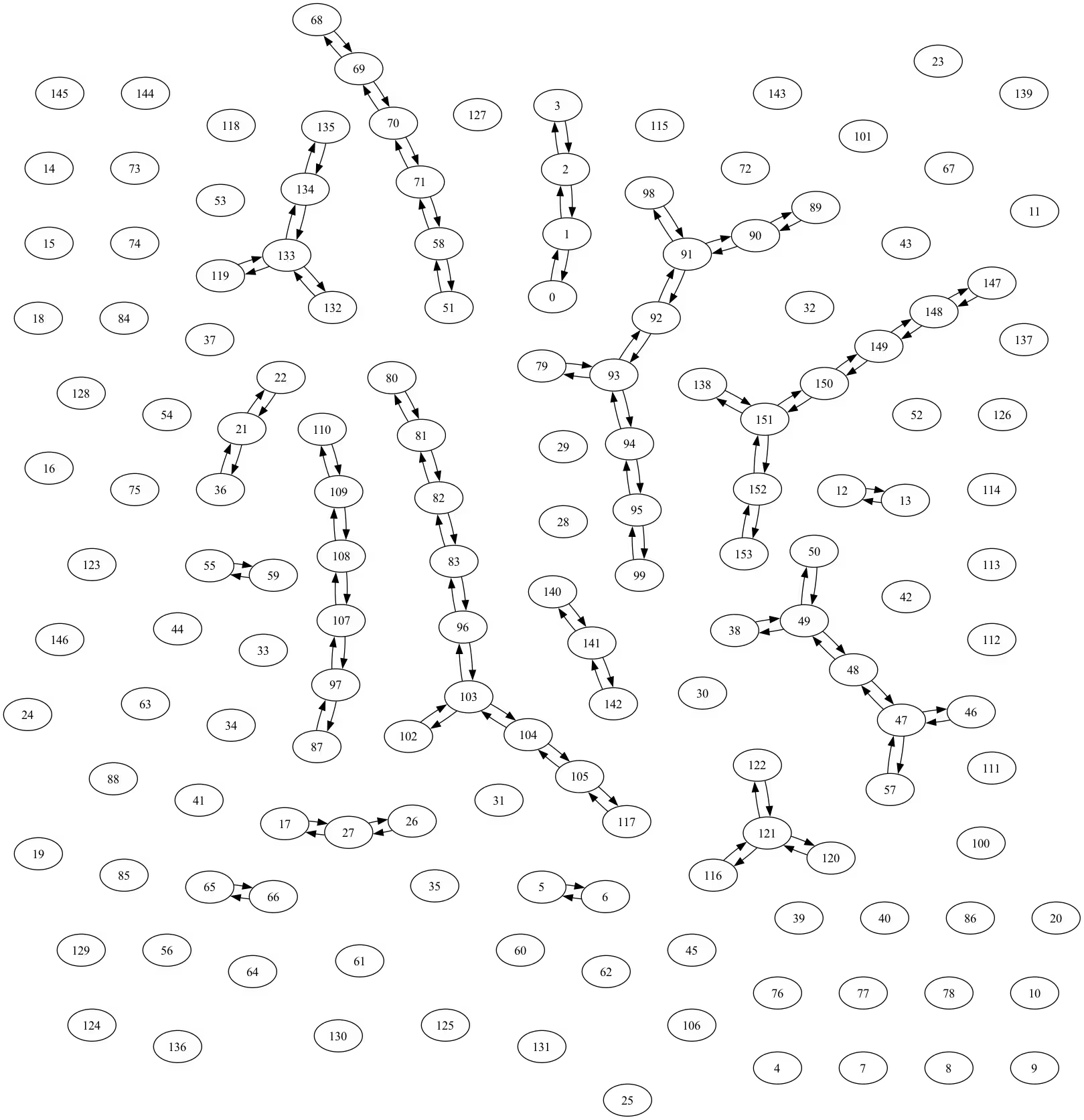
สำหรับตัวอย่างขนาดใหญ่ เราใช้โมเดล XXZ บนเส้นตรงขนาด 50 ไซต์:

$$\hat{\mathcal{H}}_{XXZ} = \sum_{i=1}^{L-1} J_{i,(i+1)}\left(X_i X_{(i+1)}+Y_i Y_{(i+1)}+ 2\cdot Z_i Z_{(i+1)} \right) \, ,$$

โดยที่ $J_{i,(i+1)}$ คือสัมประสิทธิ์สุ่มที่สอดคล้องกับขอบ $(i, i+1)$ นี่คือ Hamiltonian ที่ใช้ในการสาธิตที่นำเสนอในเอกสารอ้างอิง [3]

L = 50
# Generate some coupling map to use for this example
coupling_map = CouplingMap.from_line(L, bidirectional=False)
graphviz_draw(coupling_map.graph, method="circo")

import numpy as np
from qiskit.quantum_info import SparsePauliOp, Pauli

# Generate random coefficients for our XXZ Hamiltonian
np.random.seed(0)
even_edges = list(coupling_map.get_edges())[::2]
odd_edges = list(coupling_map.get_edges())[1::2]

Js = np.random.uniform(0.5, 1.5, size=L)
hamiltonian = SparsePauliOp(Pauli("I" * L))
for i, edge in enumerate(even_edges + odd_edges):
    hamiltonian += SparsePauliOp.from_sparse_list(
        [
            ("XX", (edge), 2 * Js[i]),
            ("YY", (edge), 2 * Js[i]),
            ("ZZ", (edge), 4 * Js[i]),
        ],
        num_qubits=L,
    )

print(hamiltonian)

SparsePauliOp(['IIIIIIIIIIIIIIIIIIIIIIIIIIIIIIIIIIIIIIIIIIIIIIIIII', 'IIIIIIIIIIIIIIIIIIIIIIIIIIIIIIIIIIIIIIIIIIIIIIIIXX', 'IIIIIIIIIIIIIIIIIIIIIIIIIIIIIIIIIIIIIIIIIIIIIIIIYY', 'IIIIIIIIIIIIIIIIIIIIIIIIIIIIIIIIIIIIIIIIIIIIIIIIZZ', 'IIIIIIIIIIIIIIIIIIIIIIIIIIIIIIIIIIIIIIIIIIIIIIXXII', 'IIIIIIIIIIIIIIIIIIIIIIIIIIIIIIIIIIIIIIIIIIIIIIYYII', 'IIIIIIIIIIIIIIIIIIIIIIIIIIIIIIIIIIIIIIIIIIIIIIZZII', 'IIIIIIIIIIIIIIIIIIIIIIIIIIIIIIIIIIIIIIIIIIIIXXIIII', 'IIIIIIIIIIIIIIIIIIIIIIIIIIIIIIIIIIIIIIIIIIIIYYIIII', 'IIIIIIIIIIIIIIIIIIIIIIIIIIIIIIIIIIIIIIIIIIIIZZIIII', 'IIIIIIIIIIIIIIIIIIIIIIIIIIIIIIIIIIIIIIIIIIXXIIIIII', 'IIIIIIIIIIIIIIIIIIIIIIIIIIIIIIIIIIIIIIIIIIYYIIIIII', 'IIIIIIIIIIIIIIIIIIIIIIIIIIIIIIIIIIIIIIIIIIZZIIIIII', 'IIIIIIIIIIIIIIIIIIIIIIIIIIIIIIIIIIIIIIIIXXIIIIIIII', 'IIIIIIIIIIIIIIIIIIIIIIIIIIIIIIIIIIIIIIIIYYIIIIIIII', 'IIIIIIIIIIIIIIIIIIIIIIIIIIIIIIIIIIIIIIIIZZIIIIIIII', 'IIIIIIIIIIIIIIIIIIIIIIIIIIIIIIIIIIIIIIXXIIIIIIIIII', 'IIIIIIIIIIIIIIIIIIIIIIIIIIIIIIIIIIIIIIYYIIIIIIIIII', 'IIIIIIIIIIIIIIIIIIIIIIIIIIIIIIIIIIIIIIZZIIIIIIIIII', 'IIIIIIIIIIIIIIIIIIIIIIIIIIIIIIIIIIIIXXIIIIIIIIIIII', 'IIIIIIIIIIIIIIIIIIIIIIIIIIIIIIIIIIIIYYIIIIIIIIIIII', 'IIIIIIIIIIIIIIIIIIIIIIIIIIIIIIIIIIIIZZIIIIIIIIIIII', 'IIIIIIIIIIIIIIIIIIIIIIIIIIIIIIIIIIXXIIIIIIIIIIIIII', 'IIIIIIIIIIIIIIIIIIIIIIIIIIIIIIIIIIYYIIIIIIIIIIIIII', 'IIIIIIIIIIIIIIIIIIIIIIIIIIIIIIIIIIZZIIIIIIIIIIIIII', 'IIIIIIIIIIIIIIIIIIIIIIIIIIIIIIIIXXIIIIIIIIIIIIIIII', 'IIIIIIIIIIIIIIIIIIIIIIIIIIIIIIIIYYIIIIIIIIIIIIIIII', 'IIIIIIIIIIIIIIIIIIIIIIIIIIIIIIIIZZIIIIIIIIIIIIIIII', 'IIIIIIIIIIIIIIIIIIIIIIIIIIIIIIXXIIIIIIIIIIIIIIIIII', 'IIIIIIIIIIIIIIIIIIIIIIIIIIIIIIYYIIIIIIIIIIIIIIIIII', 'IIIIIIIIIIIIIIIIIIIIIIIIIIIIIIZZIIIIIIIIIIIIIIIIII', 'IIIIIIIIIIIIIIIIIIIIIIIIIIIIXXIIIIIIIIIIIIIIIIIIII', 'IIIIIIIIIIIIIIIIIIIIIIIIIIIIYYIIIIIIIIIIIIIIIIIIII', 'IIIIIIIIIIIIIIIIIIIIIIIIIIIIZZIIIIIIIIIIIIIIIIIIII', 'IIIIIIIIIIIIIIIIIIIIIIIIIIXXIIIIIIIIIIIIIIIIIIIIII', 'IIIIIIIIIIIIIIIIIIIIIIIIIIYYIIIIIIIIIIIIIIIIIIIIII', 'IIIIIIIIIIIIIIIIIIIIIIIIIIZZIIIIIIIIIIIIIIIIIIIIII', 'IIIIIIIIIIIIIIIIIIIIIIIIXXIIIIIIIIIIIIIIIIIIIIIIII', 'IIIIIIIIIIIIIIIIIIIIIIIIYYIIIIIIIIIIIIIIIIIIIIIIII', 'IIIIIIIIIIIIIIIIIIIIIIIIZZIIIIIIIIIIIIIIIIIIIIIIII', 'IIIIIIIIIIIIIIIIIIIIIIXXIIIIIIIIIIIIIIIIIIIIIIIIII', 'IIIIIIIIIIIIIIIIIIIIIIYYIIIIIIIIIIIIIIIIIIIIIIIIII', 'IIIIIIIIIIIIIIIIIIIIIIZZIIIIIIIIIIIIIIIIIIIIIIIIII', 'IIIIIIIIIIIIIIIIIIIIXXIIIIIIIIIIIIIIIIIIIIIIIIIIII', 'IIIIIIIIIIIIIIIIIIIIYYIIIIIIIIIIIIIIIIIIIIIIIIIIII', 'IIIIIIIIIIIIIIIIIIIIZZIIIIIIIIIIIIIIIIIIIIIIIIIIII', 'IIIIIIIIIIIIIIIIIIXXIIIIIIIIIIIIIIIIIIIIIIIIIIIIII', 'IIIIIIIIIIIIIIIIIIYYIIIIIIIIIIIIIIIIIIIIIIIIIIIIII', 'IIIIIIIIIIIIIIIIIIZZIIIIIIIIIIIIIIIIIIIIIIIIIIIIII', 'IIIIIIIIIIIIIIIIXXIIIIIIIIIIIIIIIIIIIIIIIIIIIIIIII', 'IIIIIIIIIIIIIIIIYYIIIIIIIIIIIIIIIIIIIIIIIIIIIIIIII', 'IIIIIIIIIIIIIIIIZZIIIIIIIIIIIIIIIIIIIIIIIIIIIIIIII', 'IIIIIIIIIIIIIIXXIIIIIIIIIIIIIIIIIIIIIIIIIIIIIIIIII', 'IIIIIIIIIIIIIIYYIIIIIIIIIIIIIIIIIIIIIIIIIIIIIIIIII', 'IIIIIIIIIIIIIIZZIIIIIIIIIIIIIIIIIIIIIIIIIIIIIIIIII', 'IIIIIIIIIIIIXXIIIIIIIIIIIIIIIIIIIIIIIIIIIIIIIIIIII', 'IIIIIIIIIIIIYYIIIIIIIIIIIIIIIIIIIIIIIIIIIIIIIIIIII', 'IIIIIIIIIIIIZZIIIIIIIIIIIIIIIIIIIIIIIIIIIIIIIIIIII', 'IIIIIIIIIIXXIIIIIIIIIIIIIIIIIIIIIIIIIIIIIIIIIIIIII', 'IIIIIIIIIIYYIIIIIIIIIIIIIIIIIIIIIIIIIIIIIIIIIIIIII', 'IIIIIIIIIIZZIIIIIIIIIIIIIIIIIIIIIIIIIIIIIIIIIIIIII', 'IIIIIIIIXXIIIIIIIIIIIIIIIIIIIIIIIIIIIIIIIIIIIIIIII', 'IIIIIIIIYYIIIIIIIIIIIIIIIIIIIIIIIIIIIIIIIIIIIIIIII', 'IIIIIIIIZZIIIIIIIIIIIIIIIIIIIIIIIIIIIIIIIIIIIIIIII', 'IIIIIIXXIIIIIIIIIIIIIIIIIIIIIIIIIIIIIIIIIIIIIIIIII', 'IIIIIIYYIIIIIIIIIIIIIIIIIIIIIIIIIIIIIIIIIIIIIIIIII', 'IIIIIIZZIIIIIIIIIIIIIIIIIIIIIIIIIIIIIIIIIIIIIIIIII', 'IIIIXXIIIIIIIIIIIIIIIIIIIIIIIIIIIIIIIIIIIIIIIIIIII', 'IIIIYYIIIIIIIIIIIIIIIIIIIIIIIIIIIIIIIIIIIIIIIIIIII', 'IIIIZZIIIIIIIIIIIIIIIIIIIIIIIIIIIIIIIIIIIIIIIIIIII', 'IIXXIIIIIIIIIIIIIIIIIIIIIIIIIIIIIIIIIIIIIIIIIIIIII', 'IIYYIIIIIIIIIIIIIIIIIIIIIIIIIIIIIIIIIIIIIIIIIIIIII', 'IIZZIIIIIIIIIIIIIIIIIIIIIIIIIIIIIIIIIIIIIIIIIIIIII', 'XXIIIIIIIIIIIIIIIIIIIIIIIIIIIIIIIIIIIIIIIIIIIIIIII', 'YYIIIIIIIIIIIIIIIIIIIIIIIIIIIIIIIIIIIIIIIIIIIIIIII', 'ZZIIIIIIIIIIIIIIIIIIIIIIIIIIIIIIIIIIIIIIIIIIIIIIII', 'IIIIIIIIIIIIIIIIIIIIIIIIIIIIIIIIIIIIIIIIIIIIIIIXXI', 'IIIIIIIIIIIIIIIIIIIIIIIIIIIIIIIIIIIIIIIIIIIIIIIYYI', 'IIIIIIIIIIIIIIIIIIIIIIIIIIIIIIIIIIIIIIIIIIIIIIIZZI', 'IIIIIIIIIIIIIIIIIIIIIIIIIIIIIIIIIIIIIIIIIIIIIXXIII', 'IIIIIIIIIIIIIIIIIIIIIIIIIIIIIIIIIIIIIIIIIIIIIYYIII', 'IIIIIIIIIIIIIIIIIIIIIIIIIIIIIIIIIIIIIIIIIIIIIZZIII', 'IIIIIIIIIIIIIIIIIIIIIIIIIIIIIIIIIIIIIIIIIIIXXIIIII', 'IIIIIIIIIIIIIIIIIIIIIIIIIIIIIIIIIIIIIIIIIIIYYIIIII', 'IIIIIIIIIIIIIIIIIIIIIIIIIIIIIIIIIIIIIIIIIIIZZIIIII', 'IIIIIIIIIIIIIIIIIIIIIIIIIIIIIIIIIIIIIIIIIXXIIIIIII', 'IIIIIIIIIIIIIIIIIIIIIIIIIIIIIIIIIIIIIIIIIYYIIIIIII', 'IIIIIIIIIIIIIIIIIIIIIIIIIIIIIIIIIIIIIIIIIZZIIIIIII', 'IIIIIIIIIIIIIIIIIIIIIIIIIIIIIIIIIIIIIIIXXIIIIIIIII', 'IIIIIIIIIIIIIIIIIIIIIIIIIIIIIIIIIIIIIIIYYIIIIIIIII', 'IIIIIIIIIIIIIIIIIIIIIIIIIIIIIIIIIIIIIIIZZIIIIIIIII', 'IIIIIIIIIIIIIIIIIIIIIIIIIIIIIIIIIIIIIXXIIIIIIIIIII', 'IIIIIIIIIIIIIIIIIIIIIIIIIIIIIIIIIIIIIYYIIIIIIIIIII', 'IIIIIIIIIIIIIIIIIIIIIIIIIIIIIIIIIIIIIZZIIIIIIIIIII', 'IIIIIIIIIIIIIIIIIIIIIIIIIIIIIIIIIIIXXIIIIIIIIIIIII', 'IIIIIIIIIIIIIIIIIIIIIIIIIIIIIIIIIIIYYIIIIIIIIIIIII', 'IIIIIIIIIIIIIIIIIIIIIIIIIIIIIIIIIIIZZIIIIIIIIIIIII', 'IIIIIIIIIIIIIIIIIIIIIIIIIIIIIIIIIXXIIIIIIIIIIIIIII', 'IIIIIIIIIIIIIIIIIIIIIIIIIIIIIIIIIYYIIIIIIIIIIIIIII', 'IIIIIIIIIIIIIIIIIIIIIIIIIIIIIIIIIZZIIIIIIIIIIIIIII', 'IIIIIIIIIIIIIIIIIIIIIIIIIIIIIIIXXIIIIIIIIIIIIIIIII', 'IIIIIIIIIIIIIIIIIIIIIIIIIIIIIIIYYIIIIIIIIIIIIIIIII', 'IIIIIIIIIIIIIIIIIIIIIIIIIIIIIIIZZIIIIIIIIIIIIIIIII', 'IIIIIIIIIIIIIIIIIIIIIIIIIIIIIXXIIIIIIIIIIIIIIIIIII', 'IIIIIIIIIIIIIIIIIIIIIIIIIIIIIYYIIIIIIIIIIIIIIIIIII', 'IIIIIIIIIIIIIIIIIIIIIIIIIIIIIZZIIIIIIIIIIIIIIIIIII', 'IIIIIIIIIIIIIIIIIIIIIIIIIIIXXIIIIIIIIIIIIIIIIIIIII', 'IIIIIIIIIIIIIIIIIIIIIIIIIIIYYIIIIIIIIIIIIIIIIIIIII', 'IIIIIIIIIIIIIIIIIIIIIIIIIIIZZIIIIIIIIIIIIIIIIIIIII', 'IIIIIIIIIIIIIIIIIIIIIIIIIXXIIIIIIIIIIIIIIIIIIIIIII', 'IIIIIIIIIIIIIIIIIIIIIIIIIYYIIIIIIIIIIIIIIIIIIIIIII', 'IIIIIIIIIIIIIIIIIIIIIIIIIZZIIIIIIIIIIIIIIIIIIIIIII', 'IIIIIIIIIIIIIIIIIIIIIIIXXIIIIIIIIIIIIIIIIIIIIIIIII', 'IIIIIIIIIIIIIIIIIIIIIIIYYIIIIIIIIIIIIIIIIIIIIIIIII', 'IIIIIIIIIIIIIIIIIIIIIIIZZIIIIIIIIIIIIIIIIIIIIIIIII', 'IIIIIIIIIIIIIIIIIIIIIXXIIIIIIIIIIIIIIIIIIIIIIIIIII', 'IIIIIIIIIIIIIIIIIIIIIYYIIIIIIIIIIIIIIIIIIIIIIIIIII', 'IIIIIIIIIIIIIIIIIIIIIZZIIIIIIIIIIIIIIIIIIIIIIIIIII', 'IIIIIIIIIIIIIIIIIIIXXIIIIIIIIIIIIIIIIIIIIIIIIIIIII', 'IIIIIIIIIIIIIIIIIIIYYIIIIIIIIIIIIIIIIIIIIIIIIIIIII', 'IIIIIIIIIIIIIIIIIIIZZIIIIIIIIIIIIIIIIIIIIIIIIIIIII', 'IIIIIIIIIIIIIIIIIXXIIIIIIIIIIIIIIIIIIIIIIIIIIIIIII', 'IIIIIIIIIIIIIIIIIYYIIIIIIIIIIIIIIIIIIIIIIIIIIIIIII', 'IIIIIIIIIIIIIIIIIZZIIIIIIIIIIIIIIIIIIIIIIIIIIIIIII', 'IIIIIIIIIIIIIIIXXIIIIIIIIIIIIIIIIIIIIIIIIIIIIIIIII', 'IIIIIIIIIIIIIIIYYIIIIIIIIIIIIIIIIIIIIIIIIIIIIIIIII', 'IIIIIIIIIIIIIIIZZIIIIIIIIIIIIIIIIIIIIIIIIIIIIIIIII', 'IIIIIIIIIIIIIXXIIIIIIIIIIIIIIIIIIIIIIIIIIIIIIIIIII', 'IIIIIIIIIIIIIYYIIIIIIIIIIIIIIIIIIIIIIIIIIIIIIIIIII', 'IIIIIIIIIIIIIZZIIIIIIIIIIIIIIIIIIIIIIIIIIIIIIIIIII', 'IIIIIIIIIIIXXIIIIIIIIIIIIIIIIIIIIIIIIIIIIIIIIIIIII', 'IIIIIIIIIIIYYIIIIIIIIIIIIIIIIIIIIIIIIIIIIIIIIIIIII', 'IIIIIIIIIIIZZIIIIIIIIIIIIIIIIIIIIIIIIIIIIIIIIIIIII', 'IIIIIIIIIXXIIIIIIIIIIIIIIIIIIIIIIIIIIIIIIIIIIIIIII', 'IIIIIIIIIYYIIIIIIIIIIIIIIIIIIIIIIIIIIIIIIIIIIIIIII', 'IIIIIIIIIZZIIIIIIIIIIIIIIIIIIIIIIIIIIIIIIIIIIIIIII', 'IIIIIIIXXIIIIIIIIIIIIIIIIIIIIIIIIIIIIIIIIIIIIIIIII', 'IIIIIIIYYIIIIIIIIIIIIIIIIIIIIIIIIIIIIIIIIIIIIIIIII', 'IIIIIIIZZIIIIIIIIIIIIIIIIIIIIIIIIIIIIIIIIIIIIIIIII', 'IIIIIXXIIIIIIIIIIIIIIIIIIIIIIIIIIIIIIIIIIIIIIIIIII', 'IIIIIYYIIIIIIIIIIIIIIIIIIIIIIIIIIIIIIIIIIIIIIIIIII', 'IIIIIZZIIIIIIIIIIIIIIIIIIIIIIIIIIIIIIIIIIIIIIIIIII', 'IIIXXIIIIIIIIIIIIIIIIIIIIIIIIIIIIIIIIIIIIIIIIIIIII', 'IIIYYIIIIIIIIIIIIIIIIIIIIIIIIIIIIIIIIIIIIIIIIIIIII', 'IIIZZIIIIIIIIIIIIIIIIIIIIIIIIIIIIIIIIIIIIIIIIIIIII', 'IXXIIIIIIIIIIIIIIIIIIIIIIIIIIIIIIIIIIIIIIIIIIIIIII', 'IYYIIIIIIIIIIIIIIIIIIIIIIIIIIIIIIIIIIIIIIIIIIIIIII', 'IZZIIIIIIIIIIIIIIIIIIIIIIIIIIIIIIIIIIIIIIIIIIIIIII'],
              coeffs=[1.        +0.j, 2.09762701+0.j, 2.09762701+0.j, 4.19525402+0.j,
 2.43037873+0.j, 2.43037873+0.j, 4.86075747+0.j, 2.20552675+0.j,
 2.20552675+0.j, 4.4110535 +0.j, 2.08976637+0.j, 2.08976637+0.j,
 4.17953273+0.j, 1.8473096 +0.j, 1.8473096 +0.j, 3.6946192 +0.j,
 2.29178823+0.j, 2.29178823+0.j, 4.58357645+0.j, 1.87517442+0.j,
 1.87517442+0.j, 3.75034885+0.j, 2.783546  +0.j, 2.783546  +0.j,
 5.567092  +0.j, 2.92732552+0.j, 2.92732552+0.j, 5.85465104+0.j,
 1.76688304+0.j, 1.76688304+0.j, 3.53376608+0.j, 2.58345008+0.j,
 2.58345008+0.j, 5.16690015+0.j, 2.05778984+0.j, 2.05778984+0.j,
 4.11557968+0.j, 2.13608912+0.j, 2.13608912+0.j, 4.27217824+0.j,
 2.85119328+0.j, 2.85119328+0.j, 5.70238655+0.j, 1.14207212+0.j,
 1.14207212+0.j, 2.28414423+0.j, 1.1742586 +0.j, 1.1742586 +0.j,
 2.3485172 +0.j, 1.04043679+0.j, 1.04043679+0.j, 2.08087359+0.j,
 2.66523969+0.j, 2.66523969+0.j, 5.33047938+0.j, 2.5563135 +0.j,
 2.5563135 +0.j, 5.112627  +0.j, 2.7400243 +0.j, 2.7400243 +0.j,
 5.48004859+0.j, 2.95723668+0.j, 2.95723668+0.j, 5.91447337+0.j,
 2.59831713+0.j, 2.59831713+0.j, 5.19663426+0.j, 1.92295872+0.j,
 1.92295872+0.j, 3.84591745+0.j, 2.56105835+0.j, 2.56105835+0.j,
 5.12211671+0.j, 1.23654885+0.j, 1.23654885+0.j, 2.4730977 +0.j,
 2.27984204+0.j, 2.27984204+0.j, 4.55968409+0.j, 1.28670657+0.j,
 1.28670657+0.j, 2.57341315+0.j, 2.88933783+0.j, 2.88933783+0.j,
 5.77867567+0.j, 2.04369664+0.j, 2.04369664+0.j, 4.08739329+0.j,
 1.82932388+0.j, 1.82932388+0.j, 3.65864776+0.j, 1.52911122+0.j,
 1.52911122+0.j, 3.05822245+0.j, 2.54846738+0.j, 2.54846738+0.j,
 5.09693476+0.j, 1.91230066+0.j, 1.91230066+0.j, 3.82460133+0.j,
 2.1368679 +0.j, 2.1368679 +0.j, 4.2737358 +0.j, 1.0375796 +0.j,
 1.0375796 +0.j, 2.0751592 +0.j, 2.23527099+0.j, 2.23527099+0.j,
 4.47054199+0.j, 2.22419145+0.j, 2.22419145+0.j, 4.44838289+0.j,
 2.23386799+0.j, 2.23386799+0.j, 4.46773599+0.j, 2.88749616+0.j,
 2.88749616+0.j, 5.77499231+0.j, 2.3636406 +0.j, 2.3636406 +0.j,
 4.7272812 +0.j, 1.7190158 +0.j, 1.7190158 +0.j, 3.4380316 +0.j,
 1.87406391+0.j, 1.87406391+0.j, 3.74812782+0.j, 2.39526239+0.j,
 2.39526239+0.j, 4.79052478+0.j, 1.12045094+0.j, 1.12045094+0.j,
 2.24090189+0.j, 2.33353343+0.j, 2.33353343+0.j, 4.66706686+0.j,
 2.34127574+0.j, 2.34127574+0.j, 4.68255148+0.j, 1.42076512+0.j,
 1.42076512+0.j, 2.84153024+0.j, 1.2578526 +0.j, 1.2578526 +0.j,
 2.51570519+0.j, 1.6308567 +0.j, 1.6308567 +0.j, 3.2617134 +0.j])

สำหรับตัวสังเกต เราเลือก $Z_{24}Z_{25}$ ตามที่เห็นในแผงล่างของรูปที่ 5 ในเอกสารอ้างอิง [3]

observable = SparsePauliOp.from_sparse_list(
    [("ZZ", (L // 2 - 1, L // 2), 1.0)], num_qubits=L
)
print(observable)

SparsePauliOp(['IIIIIIIIIIIIIIIIIIIIIIIIZZIIIIIIIIIIIIIIIIIIIIIIII'],
              coeffs=[1.+0.j])

เลือกจำนวน Trotter steps

การทดลองที่แสดงในรูปที่ 4 ของเอกสารอ้างอิง [3] ใช้ $k_j = [2, 3, 4]$ Trotter steps แบบสมมาตรของอันดับ $2$ เราโฟกัสที่ผลลัพธ์สำหรับเวลา $t=3$ ซึ่ง MPF และ PF ที่มีจำนวน Trotter steps สูงกว่า (6 ในกรณีนี้) มี Trotter error เท่ากัน แต่ค่าคาดหวัง MPF คำนวณจาก Circuit ที่ตรงกับจำนวน Trotter steps ที่น้อยกว่าและจึงตื้นกว่า ในทางปฏิบัติ แม้ว่า MPF และ Circuit ของ Trotter steps ที่ลึกกว่าจะมี Trotter error เท่ากัน เราก็คาดว่าค่าคาดหวังเชิงทดลองที่คำนวณจาก Circuit ของ MPF จะใกล้เคียงกับทฤษฎีมากกว่า เนื่องจากการรัน Circuit ที่ตื้นกว่าจะถูกรบกวนจากสัญญาณรบกวนของฮาร์ดแวร์น้อยกว่าเมื่อเปรียบเทียบกับ Circuit ของ PF ที่มี Trotter steps สูงกว่า

total_time = 3
mpf_trotter_steps = [2, 3, 4]
order = 2
symmetric = True

ตั้งค่า LSE

ที่นี่เราดู MPF coefficients แบบ static สำหรับปัญหานี้

lse = setup_static_lse(mpf_trotter_steps, order=order, symmetric=symmetric)
mpf_coeffs = lse.solve()
print(
    f"The static coefficients associated with the ansatze are: {mpf_coeffs}"
)
print("L1 norm:", np.linalg.norm(mpf_coeffs, ord=1))

The static coefficients associated with the ansatze are: [ 0.26666667 -2.31428571  3.04761905]
L1 norm: 5.628571428571431

model_approx, coeffs_approx = setup_sum_of_squares_problem(
    lse, max_l1_norm=2.0
)
model_approx.solve()
print(coeffs_approx.value)
print(
    "L1 norm of the approximate coefficients:",
    np.linalg.norm(coeffs_approx.value, ord=1),
)

[-0.24255546 -0.25744454  1.5       ]
L1 norm of the approximate coefficients: 2.0

Dynamic coefficients

# Create approximate time-evolution circuits
single_2nd_order_circ = generate_time_evolution_circuit(
    hamiltonian, time=1.0, synthesis=SuzukiTrotter(reps=1, order=order)
)
single_2nd_order_circ = pm.run(single_2nd_order_circ)  # collect XX and YY

# Find layers in the circuit
layers = slice_by_depth(single_2nd_order_circ, max_slice_depth=1)

# Create tensor network models
models = [
    LayerModel.from_quantum_circuit(layer, conserve="Sz") for layer in layers
]

# Create the time-evolution object
approx_factory = partial(
    LayerwiseEvolver,
    layers=models,
    options={
        "preserve_norm": False,
        "trunc_params": {
            "chi_max": 64,
            "svd_min": 1e-8,
            "trunc_cut": None,
        },
        "max_delta_t": 4,
    },
)

# Create exact time-evolution circuits
single_4th_order_circ = generate_time_evolution_circuit(
    hamiltonian, time=1.0, synthesis=SuzukiTrotter(reps=1, order=4)
)
single_4th_order_circ = pm.run(single_4th_order_circ)
exact_model_layers = [
    LayerModel.from_quantum_circuit(layer, conserve="Sz")
    for layer in slice_by_depth(single_4th_order_circ, max_slice_depth=1)
]

# Create the time-evolution object
exact_factory = partial(
    LayerwiseEvolver,
    layers=exact_model_layers,
    dt=0.1,
    options={
        "preserve_norm": False,
        "trunc_params": {
            "chi_max": 64,
            "svd_min": 1e-8,
            "trunc_cut": None,
        },
        "max_delta_t": 3,
    },
)

def identity_factory():
    return MPOState.initialize_from_lattice(models[0].lat, conserve=True)

mps_initial_state = MPS_neel_state(models[0].lat)

lse = setup_dynamic_lse(
    mpf_trotter_steps,
    total_time,
    identity_factory,
    exact_factory,
    approx_factory,
    mps_initial_state,
)
problem, coeffs = setup_frobenius_problem(lse)
try:
    problem.solve()
    mpf_dynamic_coeffs = coeffs.value
except Exception as error:
    print(error, "Calculation Failed for time", total_time)
print("")

สร้าง Trotter Circuit แต่ละตัวในการแยกส่วน MPF ของเรา

from qiskit.synthesis import SuzukiTrotter
from qiskit_addon_utils.problem_generators import (
    generate_time_evolution_circuit,
)
from qiskit import QuantumCircuit

mpf_circuits = []
for k in mpf_trotter_steps:
    # Initial state preparation |1010..>
    circuit = QuantumCircuit(L)
    circuit.x([i for i in range(L) if i % 2])

    trotter_circ = generate_time_evolution_circuit(
        hamiltonian,
        synthesis=SuzukiTrotter(reps=k, order=order),
        time=total_time,
    )

    circuit.compose(trotter_circ, qubits=range(L), inplace=True)

    mpf_circuits.append(circuit)

สร้าง Trotter Circuit ที่มี Trotter error เทียบเท่ากับ MPF

k = 6

# Initial state preparation |1010..>
comp_circuit = QuantumCircuit(L)
comp_circuit.x([i for i in range(L) if i % 2])

trotter_circ = generate_time_evolution_circuit(
    hamiltonian,
    synthesis=SuzukiTrotter(reps=k, order=order),
    time=total_time,
)

comp_circuit.compose(trotter_circ, qubits=range(L), inplace=True)

mpf_circuits.append(comp_circuit)

ขั้นตอนที่ 2: ปรับแต่งปัญหาเพื่อรันบนฮาร์ดแวร์ควอนตัม

import copy
from qiskit.transpiler import Target, CouplingMap

target = backend.target
instruction_2q = "cz"

cmap = target.build_coupling_map(filter_idle_qubits=True)
cmap_list = list(cmap.get_edges())

max_meas_err = 0.055
min_t2 = 30
max_twoq_err = 0.01

# Remove qubits with bad measurement or t2
cust_cmap_list = copy.deepcopy(cmap_list)
for q in range(target.num_qubits):
    meas_err = target["measure"][(q,)].error
    if target.qubit_properties[q].t2 is not None:
        t2 = target.qubit_properties[q].t2 * 1e6
    else:
        t2 = 0
    if meas_err > max_meas_err or t2 < min_t2:
        # print(q)
        for q_pair in cmap_list:
            if q in q_pair:
                try:
                    cust_cmap_list.remove(q_pair)
                except ValueError:
                    continue

# Remove qubits with bad 2q gate or t2
for q in cmap_list:
    twoq_gate_err = target[instruction_2q][q].error
    if twoq_gate_err > max_twoq_err:
        # print(q)
        for q_pair in cmap_list:
            if q == q_pair:
                try:
                    cust_cmap_list.remove(q_pair)
                except ValueError:
                    continue

cust_cmap = CouplingMap(cust_cmap_list)

cust_target = Target.from_configuration(
    basis_gates=backend.configuration().basis_gates
    + ["measure"],  # or whatever new set of gates
    coupling_map=cust_cmap,
)

sorted_components = sorted(
    [list(comp.physical_qubits) for comp in cust_cmap.connected_components()],
    reverse=True,
)
print("size of largest component", len(sorted_components[0]))

size of largest component 73

from qiskit.transpiler.preset_passmanagers import generate_preset_pass_manager

transpiler = generate_preset_pass_manager(
    optimization_level=3, target=cust_target
)

transpiled_circuits = [transpiler.run(circ) for circ in mpf_circuits]

qubits_layouts = [
    [
        idx
        for idx, qb in circuit.layout.initial_layout.get_physical_bits().items()
        if qb._register.name != "ancilla"
    ]
    for circuit in transpiled_circuits
]

transpiled_circuits = []
for circuit, layout in zip(mpf_circuits, qubits_layouts):
    transpiler = generate_preset_pass_manager(
        optimization_level=3, backend=backend, initial_layout=layout
    )
    transpiled_circuit = transpiler.run(circuit)
    transpiled_circuits.append(transpiled_circuit)

# transform the observable defined on virtual qubits to
# an observable defined on all physical qubits
isa_observables = [
    observable.apply_layout(circ.layout) for circ in transpiled_circuits
]

ขั้นตอนที่ 3: รันด้วย Qiskit primitives

from qiskit_ibm_runtime import EstimatorV2 as Estimator

estimator = Estimator(mode=backend)
estimator.options.default_shots = 30000

# Set simple error suppression/mitigation options
estimator.options.dynamical_decoupling.enable = True
estimator.options.twirling.enable_gates = True
estimator.options.twirling.enable_measure = True
estimator.options.twirling.num_randomizations = "auto"
estimator.options.twirling.strategy = "active-accum"
estimator.options.resilience.measure_mitigation = True
estimator.options.experimental.execution_path = "gen3-turbo"

estimator.options.resilience.zne_mitigation = True
estimator.options.resilience.zne.noise_factors = (1, 1.2, 1.4)
estimator.options.resilience.zne.extrapolator = "linear"

estimator.options.environment.job_tags = ["mpf large"]

job_50 = estimator.run(
    [
        (circ, observable)
        for circ, observable in zip(transpiled_circuits, isa_observables)
    ]
)

ขั้นตอนที่ 4: ประมวลผลหลังการรันและแสดงผลลัพธ์ในรูปแบบคลาสสิกที่ต้องการ

result = job_50.result()
evs = [res.data.evs for res in result]
std = [res.data.stds for res in result]

print(evs)
print(std)

[array(-0.08034071), array(-0.00605026), array(-0.15345759), array(-0.18127293)]
[array(0.04482517), array(0.03438413), array(0.21540776), array(0.21520829)]

exact_mpf_std = np.sqrt(
    sum([(coeff**2) * (std**2) for coeff, std in zip(mpf_coeffs, std[:3])])
)
print(
    "Exact static MPF expectation value: ",
    evs[:3] @ mpf_coeffs,
    "+-",
    exact_mpf_std,
)
approx_mpf_std = np.sqrt(
    sum(
        [
            (coeff**2) * (std**2)
            for coeff, std in zip(coeffs_approx.value, std[:3])
        ]
    )
)
print(
    "Approximate static MPF expectation value: ",
    evs[:3] @ coeffs_approx.value,
    "+-",
    approx_mpf_std,
)
dynamic_mpf_std = np.sqrt(
    sum(
        [
            (coeff**2) * (std**2)
            for coeff, std in zip(mpf_dynamic_coeffs, std[:3])
        ]
    )
)
print(
    "Dynamic MPF expectation value: ",
    evs[:3] @ mpf_dynamic_coeffs,
    "+-",
    dynamic_mpf_std,
)

Exact static MPF expectation value:  -0.47510243192011536 +- 0.6613940032465087
Approximate static MPF expectation value:  -0.20914170384216998 +- 0.32341567460419135
Dynamic MPF expectation value:  -0.07994951978722761 +- 0.07423091963310202

sym = {2: "^", 3: "s", 4: "p"}
# Get expectation values at all times for each Trotter step
for k, step in enumerate(mpf_trotter_steps):
    plt.errorbar(
        k,
        evs[k],
        yerr=std[k],
        alpha=0.5,
        markersize=4,
        marker=sym[step],
        color="grey",
        label=f"{mpf_trotter_steps[k]} Trotter steps",
    )

plt.errorbar(
    3,
    evs[-1],
    yerr=std[-1],
    alpha=0.5,
    markersize=8,
    marker="x",
    color="blue",
    label="6 Trotter steps",
)

plt.errorbar(
    4,
    evs[:3] @ mpf_coeffs,
    yerr=exact_mpf_std,
    markersize=4,
    marker="o",
    color="purple",
    label="Static MPF",
)

plt.errorbar(
    5,
    evs[:3] @ coeffs_approx.value,
    yerr=approx_mpf_std,
    markersize=4,
    marker="o",
    color="orange",
    label="Approximate static MPF",
)

plt.errorbar(
    6,
    evs[:3] @ mpf_dynamic_coeffs,
    yerr=dynamic_mpf_std,
    markersize=4,
    marker="o",
    color="pink",
    label="Dynamic MPF",
)

exact_obs = -0.24384471447172074  # Calculated via Tensor Network calculation
plt.axhline(
    y=exact_obs, linestyle="--", color="red", label="Exact time-evolution"
)

plt.title(
    f"Expectation values for (ZZ,{(L//2-1, L//2)}) at time {total_time} for the different methods "
)
plt.xlabel("Method")
plt.ylabel("Expectation Value")
plt.legend(loc="upper center", bbox_to_anchor=(0.5, -0.2), ncol=2)
plt.grid(alpha=0.1)
plt.tight_layout()
plt.show()

เมื่อรัน Circuit บนฮาร์ดแวร์จริง เราอาจพบกับความท้าทายเพิ่มเติมในการได้ค่า expectation value ที่แม่นยำ เนื่องจากมีสัญญาณรบกวนจากฮาร์ดแวร์ ซึ่งสิ่งนี้ไม่ได้ถูกนำมาพิจารณาในรูปแบบ MPF และอาจส่งผลเสียต่อผลลัพธ์ของ MPF ตัวอย่างเช่น อาจเป็นสาเหตุที่ dynamic coefficients ไม่สามารถให้การประมาณค่า expectation value ที่ดีกว่า approximate static coefficient ในกราฟ กล่าวคือ approximate evolver ซึ่งจำลอง approximate circuit ไม่ได้สะท้อนผลลัพธ์ที่ได้จากการรัน approximate circuit ท่ามกลางสัญญาณรบกวนของฮาร์ดแวร์อย่างแม่นยำ ด้วยเหตุนี้ จึงแนะนำให้ใช้เทคนิคลดความผิดพลาดหลายอย่างร่วมกัน เพื่อให้ได้ผลลัพธ์ที่ใกล้เคียงกับค่าอุดมคติสำหรับแต่ละ product formula มากที่สุด วิธีนี้จะแสดงให้เห็นประโยชน์ที่สม่ำเสมอจากวิธี MPF

โดยรวมแล้ว approximate static coefficients ยังคงให้ผลลัพธ์ที่แม่นยำกว่า product formula ที่มีจำนวน Trotter steps มากกว่าซึ่งมีปริมาณ Trotter error เท่ากันในสภาวะไร้สัญญาณรบกวน

นอกจากนี้ยังสำคัญที่จะต้องสังเกตว่า ในตัวอย่างที่ทำซ้ำการทดลองใน Ref. [3] จุดเวลา $t=3$ เกินขีดจำกัดที่คาดว่า PF ที่มี $k=2$ จะทำงานได้ดี ซึ่งคือ $t/k>1$ ตามที่กล่าวถึงในคู่มือนี้.

อ้างอิง

[1] Vazquez, A. C., Egger, D. J., Ochsner, D., & Woerner, S. (2023). Well-conditioned multi-product formulas for hardware-friendly Hamiltonian simulation. Quantum, 7, 1067.

[2] Zhuk, S., Robertson, N. F., & Bravyi, S. (2024). Trotter error bounds and dynamic multi-product formulas for Hamiltonian simulation. Physical Review Research, 6(3), 033309.

[3] Robertson, N. F., et al. (2024). Tensor network enhanced dynamic multiproduct formulas. arXiv preprint arXiv:2407.17405.