การย้อนกลับตัวดำเนินการ (OBP) สำหรับการประมาณค่าความคาดหวัง

ประมาณเวลาการใช้งาน: 4 นาทีบนโปรเซสเซอร์ Heron r3 (หมายเหตุ: นี่เป็นเพียงการประมาณการ เวลาจริงอาจแตกต่างกันได้)

ผลการเรียนรู้

หลังจากผ่านบทเรียนนี้ ผู้ใช้ควรเข้าใจ:

• วิธีใช้ qiskit-addon-obp เพื่อลดความลึกของ Circuit ควอนตัมแลกกับจำนวนการรัน Circuit ที่เพิ่มขึ้น
• วิธีใช้ qiskit-addon-utils เพื่อสร้าง XYZ Hamiltonian และ Circuit การวิวัฒนาการตามเวลาของมัน

ข้อกำหนดเบื้องต้น

แนะนำให้ผู้ใช้คุ้นเคยกับหัวข้อต่อไปนี้ก่อนผ่านบทเรียนนี้:

• การใช้ Estimator primitive เพื่อคำนวณค่าความคาดหวังของ observable

พื้นหลัง

การย้อนกลับตัวดำเนินการ (Operator backpropagation) คือเทคนิคที่ดูดซับการดำเนินการจากส่วนท้ายของ Circuit ควอนตัมเข้าสู่ observable ที่วัดได้ ซึ่งโดยทั่วไปจะลดความลึกของ Circuit แลกกับจำนวน term ที่เพิ่มขึ้นใน observable เป้าหมายคือย้อนกลับ Circuit ให้ได้มากที่สุดเท่าที่จะทำได้โดยไม่ให้ observable ขยายใหญ่เกินไป การนำไปใช้งานบน Qiskit มีอยู่ใน OBP Qiskit addon อ่าน เอกสาร ที่สอดคล้องกันเพื่อข้อมูลเพิ่มเติม

พิจารณา Circuit ตัวอย่างที่ต้องวัด observable $O = \sum_P c_P P$ โดยที่ $P$ คือ Pauli และ $c_P$ คือสัมประสิทธิ์ กำหนดให้ Circuit แทนด้วย unitary เดี่ยว $U$ ซึ่งสามารถแบ่งแบบ logical ได้เป็น $U = U_C U_Q$ ดังแสดงในรูปด้านล่าง

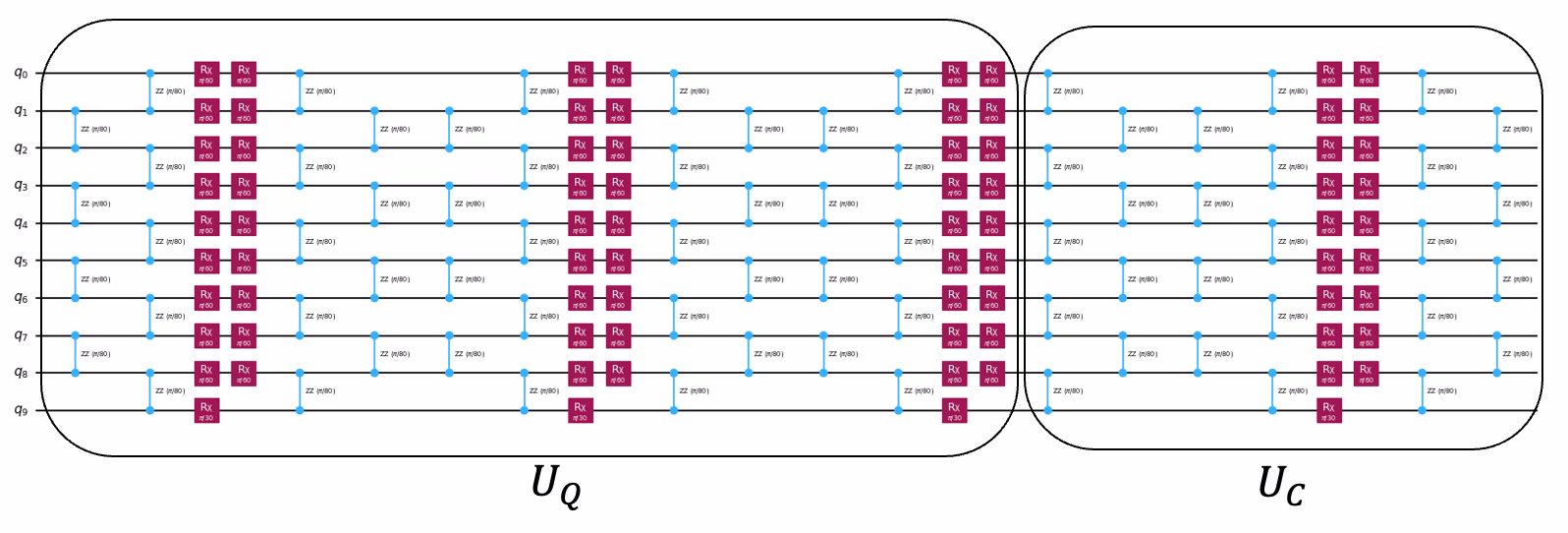
การย้อนกลับตัวดำเนินการดูดซับ unitary $U_C$ เข้าสู่ observable โดยวิวัฒนาการมันเป็น $O' = U_C^{\dagger}OU_C = \sum_P c_P U_C^{\dagger}PU_C$ พูดอีกนัยหนึ่งคือ ส่วนหนึ่งของการคำนวณดำเนินการแบบ classical ผ่านการวิวัฒนาการของ observable จาก $O$ ไปเป็น $O'$ ปัญหาเดิมสามารถกำหนดใหม่ได้เป็นการวัด observable $O'$ สำหรับ Circuit ใหม่ที่มีความลึกน้อยลง ซึ่งมี unitary เป็น $U_Q$

Unitary $U_C$ แทนด้วยจำนวน slice $U_C = U_S U_{S-1}...U_2U_1$ มีหลายวิธีในการกำหนด slice ตัวอย่างเช่น ใน Circuit ตัวอย่างข้างต้น แต่ละเลเยอร์ของ $R_{zz}$ และแต่ละเลเยอร์ของ Gate $R_x$ สามารถถือเป็น slice ได้ การย้อนกลับเกี่ยวข้องกับการคำนวณ $O' = \Pi_{s=1}^S \sum_P c_P U_s^{\dagger} P U_s$ แบบ classical โดย slice แต่ละอัน $U_s$ สามารถแทนได้เป็น $U_s = exp(\frac{-i\theta_s P_s}{2})$ โดยที่ $P_s$ คือ Pauli ขนาด $n$ Qubit และ $\theta_s$ คือสเกลาร์ สามารถตรวจสอบได้ง่ายว่า

$$U_s^{\dagger} P U_s = P \qquad \text{if} ~[P,P_s] = 0,$$ $$U_s^{\dagger} P U_s = \qquad cos(\theta_s)P + i sin(\theta_s)P_sP \qquad \text{if} ~\{P,P_s\} = 0$$

ในตัวอย่างข้างต้น ถ้า $\{P,P_s\} = 0$ เราต้องรัน Circuit ควอนตัมสอง Circuit แทนที่จะเป็นหนึ่ง Circuit เพื่อคำนวณค่าความคาดหวัง ดังนั้น การย้อนกลับอาจเพิ่มจำนวน term ใน observable ทำให้ต้องรัน Circuit มากขึ้น วิธีหนึ่งที่จะอนุญาตให้ย้อนกลับลึกกว่าเข้าไปใน Circuit โดยไม่ให้ตัวดำเนินการขยายใหญ่เกินไปคือการตัดทอน term ที่มีสัมประสิทธิ์เล็ก แทนที่จะเพิ่มลงใน operator ตัวอย่างเช่น ในตัวอย่างข้างต้น อาจเลือกตัด term ที่เกี่ยวกับ $P_sP$ ออก หากว่า $\theta_s$ เล็กพอ การตัดทอน term อาจส่งผลให้ต้องรัน Circuit ควอนตัมน้อยลง แต่จะเกิดข้อผิดพลาดบางส่วนในการคำนวณค่าความคาดหวังสุดท้ายซึ่งสัดส่วนกับขนาดของสัมประสิทธิ์ของ term ที่ถูกตัดออก

ความต้องการ

ก่อนเริ่มบทเรียนนี้ ให้แน่ใจว่าได้ติดตั้งสิ่งต่อไปนี้แล้ว:

• Qiskit SDK v2.0 หรือใหม่กว่า พร้อม visualization support
• Qiskit Runtime v0.22 หรือใหม่กว่า (pip install qiskit-ibm-runtime)
• OBP Qiskit addon 0.3 หรือใหม่กว่า (pip install qiskit-addon-obp)
• Qiskit addon utils 0.3 หรือใหม่กว่า (pip install qiskit-addon-utils)

การตั้งค่า

# Added by doQumentation — required packages for this notebook
!pip install -q matplotlib numpy qiskit qiskit-addon-obp qiskit-addon-utils qiskit-ibm-runtime rustworkx

import numpy as np
import matplotlib.pyplot as plt

from qiskit.primitives import StatevectorEstimator
from qiskit.transpiler.preset_passmanagers import generate_preset_pass_manager
from qiskit.quantum_info import SparsePauliOp
from qiskit.transpiler import CouplingMap
from qiskit.synthesis import LieTrotter

from qiskit_addon_utils.problem_generators import generate_xyz_hamiltonian
from qiskit_addon_utils.problem_generators import (
    generate_time_evolution_circuit,
)
from qiskit_addon_utils.slicing import slice_by_depth, combine_slices
from qiskit_addon_obp.utils.simplify import OperatorBudget
from qiskit_addon_obp import backpropagate
from qiskit_addon_obp.utils.truncating import setup_budget

from rustworkx.visualization import graphviz_draw

from qiskit_ibm_runtime import QiskitRuntimeService
from qiskit_ibm_runtime import EstimatorV2, EstimatorOptions

num_qubits = 10
layout = [(i - 1, i) for i in range(1, num_qubits)]

# Instantiate a CouplingMap object
coupling_map = CouplingMap(layout)
graphviz_draw(coupling_map.graph, method="circo")

ตัวอย่าง simulator ขนาดเล็ก

บทเรียนนี้นำ รูปแบบ Qiskit มาใช้จำลองพลศาสตร์ควอนตัมของโซ่สปิน Heisenberg โดยใช้ OBP Qiskit addon สังเกตว่าใน simulator ที่ไม่มี noise ค่าความคาดหวังที่ได้พร้อมและไม่พร้อม backpropagation จะเหมือนกัน

ขั้นตอนที่ 1: แมป input แบบ classical ไปสู่ปัญหาควอนตัม

แมปการวิวัฒนาการตามเวลาของโมเดลควอนตัม Heisenberg ไปสู่การทดลองควอนตัม

ก่อนอื่น เราจะใช้ฟังก์ชัน generate_xyz_hamiltonian จาก qiskit-addon-utils เพื่อสร้าง Hamiltonian แบบ Heisenberg บนกราฟการเชื่อมต่อที่กำหนด กราฟนี้สามารถเป็น rustworkx.PyGraph หรือ CouplingMap ในส่วนต่อไปนี้ เราจะใช้ CouplingMap แบบโซ่เชิงเส้นที่มี 10 Qubit

# Get a qubit operator describing the Heisenberg XYZ model
hamiltonian = generate_xyz_hamiltonian(
    coupling_map,
    coupling_constants=(np.pi / 8, np.pi / 4, np.pi / 2),
    ext_magnetic_field=(np.pi / 3, np.pi / 6, np.pi / 9),
)
print(hamiltonian)

ต่อไป เราจะสร้าง Pauli operator ที่จำลอง Hamiltonian XYZ แบบ Heisenberg:

$${\hat{\mathcal{H}}_{XYZ} = \sum_{(j,k)\in E} (J_{x} \sigma_j^{x} \sigma_{k}^{x} + J_{y} \sigma_j^{y} \sigma_{k}^{y} + J_{z} \sigma_j^{z} \sigma_{k}^{z}) + \sum_{j\in V} (h_{x} \sigma_j^{x} + h_{y} \sigma_j^{y} + h_{z} \sigma_j^{z}),}$$

โดยที่ $G(V,E)$ คือกราฟของ coupling map สำหรับบทเรียนนี้ เราใช้ $J_x, J_y, J_z$ เป็น $\frac{\pi}{8}, \frac{\pi}{4}, \frac{\pi}{2}$ ตามลำดับ และ $h_x, h_y, h_z$ เป็น $\frac{\pi}{3}, \frac{\pi}{6}, \frac{\pi}{9}$ ตามลำดับ

SparsePauliOp(['IIIIIIIXXI', 'IIIIIIIYYI', 'IIIIIIIZZI', 'IIIIIXXIII', 'IIIIIYYIII', 'IIIIIZZIII', 'IIIXXIIIII', 'IIIYYIIIII', 'IIIZZIIIII', 'IXXIIIIIII', 'IYYIIIIIII', 'IZZIIIIIII', 'IIIIIIIIXX', 'IIIIIIIIYY', 'IIIIIIIIZZ', 'IIIIIIXXII', 'IIIIIIYYII', 'IIIIIIZZII', 'IIIIXXIIII', 'IIIIYYIIII', 'IIIIZZIIII', 'IIXXIIIIII', 'IIYYIIIIII', 'IIZZIIIIII', 'XXIIIIIIII', 'YYIIIIIIII', 'ZZIIIIIIII', 'IIIIIIIIIX', 'IIIIIIIIIY', 'IIIIIIIIIZ', 'IIIIIIIIXI', 'IIIIIIIIYI', 'IIIIIIIIZI', 'IIIIIIIXII', 'IIIIIIIYII', 'IIIIIIIZII', 'IIIIIIXIII', 'IIIIIIYIII', 'IIIIIIZIII', 'IIIIIXIIII', 'IIIIIYIIII', 'IIIIIZIIII', 'IIIIXIIIII', 'IIIIYIIIII', 'IIIIZIIIII', 'IIIXIIIIII', 'IIIYIIIIII', 'IIIZIIIIII', 'IIXIIIIIII', 'IIYIIIIIII', 'IIZIIIIIII', 'IXIIIIIIII', 'IYIIIIIIII', 'IZIIIIIIII', 'XIIIIIIIII', 'YIIIIIIIII', 'ZIIIIIIIII'],
              coeffs=[0.39269908+0.j, 0.78539816+0.j, 1.57079633+0.j, 0.39269908+0.j,
 0.78539816+0.j, 1.57079633+0.j, 0.39269908+0.j, 0.78539816+0.j,
 1.57079633+0.j, 0.39269908+0.j, 0.78539816+0.j, 1.57079633+0.j,
 0.39269908+0.j, 0.78539816+0.j, 1.57079633+0.j, 0.39269908+0.j,
 0.78539816+0.j, 1.57079633+0.j, 0.39269908+0.j, 0.78539816+0.j,
 1.57079633+0.j, 0.39269908+0.j, 0.78539816+0.j, 1.57079633+0.j,
 0.39269908+0.j, 0.78539816+0.j, 1.57079633+0.j, 1.04719755+0.j,
 0.52359878+0.j, 0.34906585+0.j, 1.04719755+0.j, 0.52359878+0.j,
 0.34906585+0.j, 1.04719755+0.j, 0.52359878+0.j, 0.34906585+0.j,
 1.04719755+0.j, 0.52359878+0.j, 0.34906585+0.j, 1.04719755+0.j,
 0.52359878+0.j, 0.34906585+0.j, 1.04719755+0.j, 0.52359878+0.j,
 0.34906585+0.j, 1.04719755+0.j, 0.52359878+0.j, 0.34906585+0.j,
 1.04719755+0.j, 0.52359878+0.j, 0.34906585+0.j, 1.04719755+0.j,
 0.52359878+0.j, 0.34906585+0.j, 1.04719755+0.j, 0.52359878+0.j,
 0.34906585+0.j])

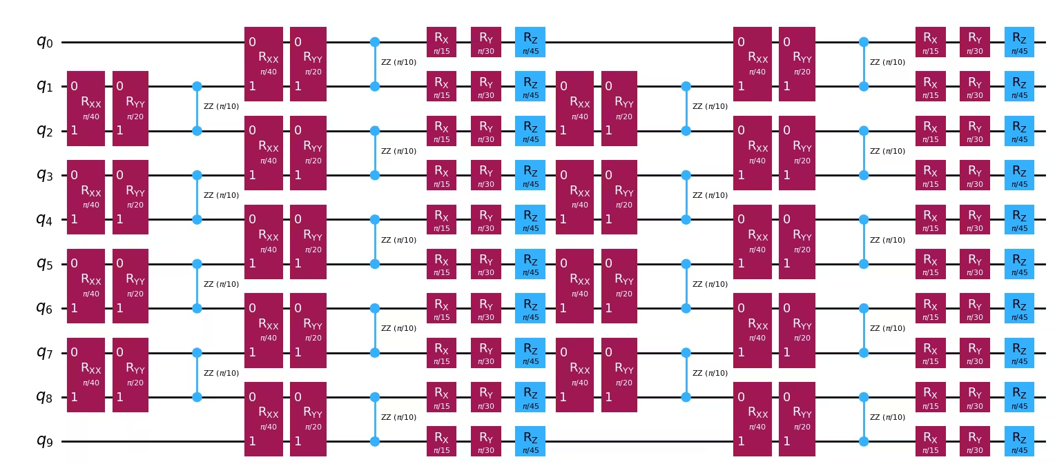
circuit = generate_time_evolution_circuit(
    hamiltonian,
    time=0.2,
    synthesis=LieTrotter(reps=2),
)
circuit.draw("mpl", style="iqp", fold=-1)

จาก qubit operator เราสามารถสร้าง Circuit ควอนตัมที่จำลองการวิวัฒนาการตามเวลาของมันได้ เราใช้ generate_time_evolution_circuit พร้อม Lie Trotter decomposition เพื่อสร้าง Circuit การวิวัฒนาการตามเวลา

slices = slice_by_depth(circuit, max_slice_depth=1)
print(f"Separated the circuit into {len(slices)} slices.")

ขั้นตอนที่ 2: ปรับปัญหาให้เหมาะสมสำหรับการรันบน hardware ควอนตัม

สร้าง slice ของ Circuit สำหรับการย้อนกลับ

ฟังก์ชัน backpropagate จะย้อนกลับ Circuit ทีละ slice ดังนั้นการเลือกวิธีตัด slice อาจมีผลต่อประสิทธิภาพของการย้อนกลับสำหรับปัญหาที่กำหนด ที่นี่เราจะจัดกลุ่ม Gate ตาม depth โดยใช้ฟังก์ชัน slice_by_depth

สำหรับการอภิปรายเพิ่มเติมเกี่ยวกับการตัด Circuit เป็น slice ดู how-to guide ของแพ็กเกจ qiskit-addon-utils

Separated the circuit into 18 slices.

op_budget = OperatorBudget(max_qwc_groups=8)

จำกัดขนาดที่ operator สามารถเติบโตได้ในระหว่างการย้อนกลับ

ในระหว่างการย้อนกลับ จำนวน term ใน operator โดยทั่วไปจะเข้าใกล้ $2^L$ อย่างรวดเร็ว โดยที่ $L$ คือจำนวน slice เมื่อ term สอง term ใน operator ไม่ commute กันแบบ qubit-wise เราต้องการ Circuit แยกกันเพื่อหาค่าความคาดหวังที่สอดคล้องกัน ตัวอย่างเช่น ถ้ามี observable สอง Qubit $O = 0.1 XX + 0.3 IZ - 0.5 IX$ เนื่องจาก $[XX,IX] = 0$ การวัดในฐานเดียวก็เพียงพอเพื่อคำนวณค่าความคาดหวังสำหรับ term สองนั้น อย่างไรก็ตาม $IZ$ anti-commute กับอีกสอง term ดังนั้นเราต้องการการวัดฐานแยกต่างหากเพื่อคำนวณค่าความคาดหวังของ $IZ$ พูดอีกนัยหนึ่งคือ เราต้องการสอง Circuit แทนที่จะเป็นหนึ่ง Circuit เพื่อคำนวณ $\langle O \rangle$ เมื่อจำนวน term ใน operator เพิ่มขึ้น จำนวนการรัน Circuit ที่ต้องการก็อาจเพิ่มขึ้นด้วย

ขนาดของ operator สามารถจำกัดได้โดยระบุ kwarg operator_budget ของฟังก์ชัน backpropagate ซึ่งรับ instance ของ OperatorBudget

เพื่อควบคุมปริมาณทรัพยากรเพิ่มเติม (จำนวนการรัน Circuit และเวลา QPU ที่ต้องการ) ที่จัดสรร เราจำกัดจำนวน qubit-wise commuting Pauli group สูงสุดที่ observable ที่ย้อนกลับแล้วจะมีได้ ที่นี่เราระบุว่าการย้อนกลับควรหยุดเมื่อจำนวน qubit-wise commuting Pauli group ใน operator เกินแปดกลุ่ม

observable = SparsePauliOp.from_sparse_list(
    [("Z", [i], 1 / num_qubits) for i in range(num_qubits)],
    num_qubits=num_qubits,
)
observable

ย้อนกลับ slice จาก Circuit

ก่อนอื่นเราระบุให้ observable เป็น $M_Z = \frac{1}{N} \sum_{i=1}^N \langle Z_i \rangle$ โดยที่ $N$ คือจำนวน Qubit เราจะย้อนกลับ slice จาก Circuit การวิวัฒนาการตามเวลาจนกว่า term ใน observable จะไม่สามารถรวมเป็นแปดกลุ่มหรือน้อยกว่าของ qubit-wise commuting Pauli group ได้อีกต่อไป

SparsePauliOp(['IIIIIIIIIZ', 'IIIIIIIIZI', 'IIIIIIIZII', 'IIIIIIZIII', 'IIIIIZIIII', 'IIIIZIIIII', 'IIIZIIIIII', 'IIZIIIIIII', 'IZIIIIIIII', 'ZIIIIIIIII'],
              coeffs=[0.1+0.j, 0.1+0.j, 0.1+0.j, 0.1+0.j, 0.1+0.j, 0.1+0.j, 0.1+0.j, 0.1+0.j,
 0.1+0.j, 0.1+0.j])

# Backpropagate slices onto the observable
bp_obs, remaining_slices, metadata = backpropagate(
    observable, slices, operator_budget=op_budget
)
# Recombine the slices remaining after backpropagation
bp_circuit = combine_slices(remaining_slices)

print(f"Backpropagated {metadata.num_backpropagated_slices} slices.")
print(
    f"New observable has {len(bp_obs.paulis)} terms, which can be combined into "
    f"{len(bp_obs.group_commuting(qubit_wise=True))} groups."
)
print(
    f"Note that backpropagating one more slice would result in "
    f"{metadata.backpropagation_history[-1].num_paulis[0]} terms "
    f"across {metadata.backpropagation_history[-1].num_qwc_groups} groups."
)
print("The remaining circuit after backpropagation looks as follows:")
bp_circuit.draw("mpl", fold=-1, scale=0.6)

ด้านล่างนี้จะเห็นว่าเราย้อนกลับ 6 slice และ term ถูกรวมเป็น 6 กลุ่มแทนที่จะเป็น 8 กลุ่ม ซึ่งหมายความว่าการย้อนกลับอีก 1 slice จะทำให้จำนวน Pauli group เกิน 8 เราสามารถยืนยันว่าเป็นเช่นนั้นโดยตรวจสอบ metadata ที่ส่งคืน นอกจากนี้ในส่วนนี้การแปลง Circuit เป็นแบบ exact คือไม่มี term ของ observable ใหม่ $O'$ ที่ถูกตัดทอนออก Circuit และ operator ที่ย้อนกลับแล้วให้ผลลัพธ์ที่เหมือนกันกับ Circuit และ operator ดั้งเดิม

Backpropagated 6 slices.
New observable has 60 terms, which can be combined into 6 groups.
Note that backpropagating one more slice would result in 114 terms across 12 groups.
The remaining circuit after backpropagation looks as follows:

service = QiskitRuntimeService()
backend = service.least_busy(
    operational=True, simulator=False, min_num_qubits=133
)
print(backend)

สำหรับตัวอย่างขนาดเล็กบน simulator เราจะไม่ใช้การตัดทอน เนื่องจากเมื่อไม่มี noise Circuit ที่มีและไม่มี backpropagation จะให้ผลลัพธ์เหมือนกัน และการตัดทอนจะทำให้ผลลัพธ์แย่ลงเนื่องจากการประมาณที่เพิ่มเข้ามา

Transpile Circuit ไปยัง basis gate set

ตอนนี้เราจะ Transpile ทั้ง Circuit ดั้งเดิมและ Circuit ที่ผ่าน backpropagation ไปยัง basis gate ของ Backend เราไม่จำเป็นต้อง Transpile บน Backend จริง เนื่องจากเราจะรันบน simulator สำหรับ instance ขนาดเล็ก

<IBMBackend('ibm_kingston')>

pm_basis = generate_preset_pass_manager(
    optimization_level=3, basis_gates=backend.configuration().basis_gates
)
isa_circuit = pm_basis.run(circuit)
isa_bp_circuit = pm_basis.run(bp_circuit)

pubs = [(isa_circuit, observable), (isa_bp_circuit, bp_obs)]

ขั้นตอนที่ 3: รันด้วย Qiskit primitives

ก่อนอื่น เราสร้าง Primitive Unified Blocs (PUB) สองอันที่สอดคล้องกับ Circuit ดั้งเดิม และ Circuit ที่ผ่าน backpropagation จากนั้นเราจะรัน PUB บน Estimator แบบ ideal เพื่อหาค่าความคาดหวัง

rng = np.random.default_rng()
estimator = StatevectorEstimator(seed=rng)
job = estimator.run(pubs)

primitive_result = job.result()
circuit_expval = primitive_result[0].data.evs.item()
bp_circuit_expval = primitive_result[1].data.evs.item()

ขั้นตอนที่ 4: ประมวลผลหลังการรันและแปลงผลลัพธ์กลับเป็นรูปแบบ classical ที่ต้องการ

ตอนนี้เราหาค่าความคาดหวังของ Circuit ดั้งเดิมและ Circuit ที่ผ่าน backpropagation

methods = [
    "No backpropagation",
    "Backpropagation",
]
values = [circuit_expval, bp_circuit_expval]

ax = plt.gca()
plt.bar(methods, values, color="#a56eff", width=0.4, edgecolor="#8a3ffc")
ax.set_ylim([0.6, 0.92])
ax.set_ylabel(r"$M_Z$", fontsize=12)

Text(0, 0.5, '$M_Z$')

num_qubits = 50
layout = [(i - 1, i) for i in range(1, num_qubits)]

# Instantiate a CouplingMap object
coupling_map = CouplingMap(layout)

hamiltonian = generate_xyz_hamiltonian(
    coupling_map,
    coupling_constants=(np.pi / 8, np.pi / 4, np.pi / 2),
    ext_magnetic_field=(np.pi / 3, np.pi / 6, np.pi / 9),
)

# Generate a time evolution circuit for the Hamiltonian
circuit = generate_time_evolution_circuit(
    hamiltonian,
    time=0.2,
    synthesis=LieTrotter(reps=4),
)

# Define the observable to measure
observable = SparsePauliOp.from_sparse_list(
    [("Z", [i], 1 / num_qubits) for i in range(num_qubits)],
    num_qubits,
)

slices = slice_by_depth(circuit, max_slice_depth=1)

# Define the maximum number of qwc groups allowed in the
# backpropagated observable,
# and the truncation error budget
op_budget = OperatorBudget(max_qwc_groups=15)
truncation_error_budget = setup_budget(
    max_error_total=0.03, max_error_per_slice=0.005
)

# First backpropagation without truncation
bp_obs, remaining_slices, metadata = backpropagate(
    observable, slices, operator_budget=op_budget
)
bp_circuit = combine_slices(remaining_slices)

# Now backpropagate with truncation, using the same operator budget and
# the defined truncation error budget
bp_obs_trunc, remaining_slices_trunc, metadata = backpropagate(
    observable,
    slices,
    operator_budget=op_budget,
    truncation_error_budget=truncation_error_budget,
)
bp_circuit_trunc = combine_slices(
    remaining_slices_trunc, include_barriers=False
)

# Now we transpile the original circuit and the two backpropagated circuits,
# and apply the layout to the corresponding observables
pm = generate_preset_pass_manager(optimization_level=3, backend=backend)

isa_circuit = pm.run(circuit)
isa_bp_circuit = pm.run(bp_circuit)
isa_bp_circuit_trunc = pm.run(bp_circuit_trunc)

isa_observable = observable.apply_layout(isa_circuit.layout)
isa_bp_observable = bp_obs.apply_layout(isa_bp_circuit.layout)
isa_bp_observable_trunc = bp_obs_trunc.apply_layout(
    isa_bp_circuit_trunc.layout
)

# Compare the 2-qubit depth of each transpiled circuit to see how much
# depth backpropagation saved
print(
    f"2-qubit depth without backpropagation: "
    f"{isa_circuit.depth(lambda x: x.operation.num_qubits == 2)}"
)
print(
    f"2-qubit depth with backpropagation: "
    f"{isa_bp_circuit.depth(lambda x: x.operation.num_qubits == 2)}"
)
print(
    f"2-qubit depth with backpropagation and truncation: "
    f"{isa_bp_circuit_trunc.depth(lambda x: x.operation.num_qubits == 2)}"
)

pubs = [
    (isa_circuit, isa_observable),
    (isa_bp_circuit, isa_bp_observable),
    (isa_bp_circuit_trunc, isa_bp_observable_trunc),
]

# Now we instantiate the Estimator primitive for the hardware with
# ZNE and measurement error
# mitigation and compute the three circuits and observables
options = EstimatorOptions()
options.default_precision = 0.01
options.resilience_level = 2
options.resilience.zne.noise_factors = [1, 1.2, 1.4]
options.resilience.zne.extrapolator = ["linear"]
estimator = EstimatorV2(mode=backend, options=options)

estimator.options.environment.job_tags = ["TUT_OBP"]
job = estimator.run(pubs)

# Retrieve the results and the standard deviations
result_no_bp = job.result()[0].data.evs.item()
result_bp = job.result()[1].data.evs.item()
result_bp_trunc = job.result()[2].data.evs.item()

std_no_bp = job.result()[0].data.stds.item()
std_bp = job.result()[1].data.stds.item()
std_bp_trunc = job.result()[2].data.stds.item()

ตามที่คาดไว้ ค่าความคาดหวังทั้งสองตรงกัน เนื่องจากเรารันบน statevector simulator ที่ไม่มี noise backpropagation เป็นการแปลงแบบ exact ของคู่ Circuit-observable ดังนั้น workflow ดั้งเดิมและที่ผ่าน backpropagation จะต้องให้ค่า $M_Z$ เหมือนกัน ประโยชน์ของ backpropagation จะปรากฏชัดเจนบน hardware จริงที่มี noise เท่านั้น ซึ่ง Circuit ที่ผ่าน backpropagation ที่สั้นกว่าจะสะสมข้อผิดพลาดน้อยกว่า ดังแสดงในตัวอย่าง hardware ขนาดใหญ่ด้านล่าง

ตัวอย่าง hardware ขนาดใหญ่

เมื่อพัฒนาการทดลอง การเริ่มด้วย Circuit ขนาดเล็กเพื่อให้การแสดงภาพและการจำลองง่ายขึ้นนั้นมีประโยชน์ ตอนนี้เราดู operator backpropagation สำหรับ Heisenberg Hamiltonian ขนาด 50 Qubit ที่มีค่า $J$ และ $h$ เหมือนกัน และ observable $M_Z$ เหมือนกัน แต่มีสี่ Trotter step ค่าความคาดหวัง ideal ในระดับนี้ไม่สามารถคำนวณด้วยวิธี brute force ดังนั้นเราใช้ tensor network และได้ค่าความคาดหวัง ideal ประมาณ $\simeq 0.89$

พร้อมกับ backpropagation ในตัวอย่างขนาดใหญ่นี้ เรายังแนะนำ backpropagation พร้อมการตัดทอน โดยอุดมคติเราต้องการย้อนกลับให้มากที่สุดเพื่อลด depth ของ Circuit ที่มีประสิทธิภาพ อย่างไรก็ตาม บ่อยครั้งจะทำให้มี term ที่ไม่ commute จำนวนมากใน observable ที่อัปเดตแล้ว ซึ่งเพิ่ม quantum overhead ดังนั้นเราจึงสามารถกำจัด term ของ observable ที่มีสัมประสิทธิ์เล็กได้โดยใช้วิธีการที่เรียกว่าการตัดทอน แม้ว่าการตัดทอนจะช่วยให้ propagation มากขึ้นโดยลดจำนวน term ใน observable ที่อัปเดต แต่ก็แนะนำการประมาณบางส่วนด้วย ดังนั้นจึงจำเป็นต้องจำกัดการตัดทอนให้อยู่ในขอบเขตบางอย่างเพื่อไม่ให้ข้อผิดพลาดจากการประมาณมีมากกว่าการลด noise ที่ได้จาก backpropagation ที่ลึกกว่า

เพื่อจำกัดปริมาณการตัดทอน เราจัดสรร error budget สำหรับแต่ละ slice รวมถึง error budget รวมตลอด Circuit ที่ผ่าน backpropagation ทั้งหมด โดยใช้ฟังก์ชัน setup_budget ซึ่งทำให้มั่นใจได้ว่าการตัดทอนถูกควบคุมทั้งในแต่ละ slice และสำหรับ Circuit ทั้งหมด ดูเพิ่มเติมที่ guide นี้สำหรับวิธีอื่นในการจัดสรร budget

2-qubit depth without backpropagation: 24
2-qubit depth with backpropagation: 20
2-qubit depth with backpropagation and truncation: 18

print(f"Expectation value without backpropagation: {result_no_bp}")
print(f"Backpropagated expectation value: {result_bp}")
print(f"Backpropagated expectation value with truncation: {result_bp_trunc}")

Expectation value without backpropagation: 0.9543907942381811
Backpropagated expectation value: 0.9445337385406468
Backpropagated expectation value with truncation: 0.934050286970965

# Plot the results
methods = [
    "No backpropagation",
    "Backpropagation",
    "Backpropagation w/ truncation",
]
values = [result_no_bp, result_bp, result_bp_trunc]
error_bars = [std_no_bp, std_bp, std_bp_trunc]

ax = plt.gca()
plt.bar(methods, values, color="#a56eff", width=0.4, edgecolor="#8a3ffc")
plt.errorbar(methods, values, yerr=error_bars, fmt="o", color="r", capsize=5)
plt.axhline(0.89)
ax.set_ylim([0.8, 0.98])
plt.text(0.25, 0.895, "Exact result")
ax.set_ylabel(r"$M_Z$", fontsize=12)

Text(0, 0.5, '$M_Z$')

ขั้นตอนถัดไป

หากคุณพบว่างานนี้น่าสนใจ คุณอาจสนใจเนื้อหาต่อไปนี้:

Recommendations

• Approximate quantum compilation for time evolution circuits
• Multi-product formulas to reduce Trotter error
• pauli-prop แพ็กเกจ Pauli propagation ที่เร่งด้วย Rust พร้อม tutorials ที่ครอบคลุม OBP การประมาณค่าความคาดหวังแบบ classical และการจำลองแบบมี noise