Circuit cutting สำหรับเงื่อนไขขอบเขตเป็นคาบ

ประมาณการใช้งาน: สองนาทีบนโปรเซสเซอร์ Eagle (หมายเหตุ: นี่เป็นเพียงการประมาณเท่านั้น เวลาจริงอาจแตกต่างกัน)

พื้นฐาน

ใน notebook นี้ เราจะพิจารณาการจำลอง periodic chain ของ Qubit ที่มี 2-qubit operation ระหว่าง Qubit ที่อยู่ติดกันทุกคู่ รวมถึง Qubit แรกและ Qubit สุดท้ายด้วย Periodic chain มักพบในปัญหาทางฟิสิกส์และเคมี เช่น Ising model และการจำลองโมเลกุล

อุปกรณ์ IBM Quantum® ในปัจจุบันเป็นแบบระนาบ สามารถฝัง periodic chain บางชนิดลงบนโทโพโลยีโดยตรงได้ในกรณีที่ Qubit แรกและ Qubit สุดท้ายเป็นเพื่อนบ้านกัน อย่างไรก็ตาม สำหรับปัญหาที่มีขนาดใหญ่พอ Qubit แรกและ Qubit สุดท้ายอาจอยู่ห่างกันมาก จึงต้องใช้ SWAP gate จำนวนมากสำหรับ 2-qubit operation ระหว่างสอง Qubit นี้ ปัญหา periodic boundary แบบนี้ได้รับการศึกษาใน บทความนี้

ใน notebook นี้ เราจะแสดงการใช้ circuit cutting เพื่อจัดการกับปัญหา periodic chain ในระดับ utility scale ที่ Qubit แรกและ Qubit สุดท้ายไม่ได้เป็นเพื่อนบ้านกัน การตัด long-range connectivity นี้ช่วยหลีกเลี่ยง SWAP gate ส่วนเกิน โดยแลกกับการรันหลาย instance ของ Circuit และการประมวลผลแบบ classical หลังจากนั้น โดยสรุป การตัดสามารถนำมาใช้เพื่อคำนวณ 2-qubit operation ระยะไกลในเชิงตรรกะได้ กล่าวอีกนัยหนึ่ง วิธีนี้นำไปสู่การเพิ่ม connectivity ของ coupling map อย่างมีประสิทธิภาพ ซึ่งช่วยลดจำนวน SWAP gate ลง

โปรดสังเกตว่ามีการตัดสองประเภท ได้แก่ การตัด wire ของ Circuit (เรียกว่า wire cutting) หรือการแทนที่ 2-qubit gate ด้วย single-qubit operation หลายตัว (เรียกว่า gate cutting) ใน notebook นี้จะเน้นที่ gate cutting สำหรับรายละเอียดเพิ่มเติมเกี่ยวกับ gate cutting ดูได้ที่ เอกสารอธิบาย ใน qiskit-addon-cutting และเอกสารอ้างอิงที่เกี่ยวข้อง สำหรับรายละเอียดเพิ่มเติมเกี่ยวกับ wire cutting ดูได้ที่บทเรียน Wire cutting สำหรับการประมาณค่า expectation values หรือบทเรียนใน qiskit-addon-cutting

ข้อกำหนด

ก่อนเริ่มบทเรียนนี้ ตรวจสอบให้แน่ใจว่าติดตั้งสิ่งต่อไปนี้แล้ว:

• Qiskit SDK v1.2 หรือสูงกว่า (pip install qiskit)
• Qiskit Runtime v0.3 หรือสูงกว่า (pip install qiskit-ibm-runtime)
• Circuit cutting Qiskit addon v.9.0 หรือสูงกว่า (pip install qiskit-addon-cutting)

ตั้งค่า

# Added by doQumentation — required packages for this notebook
!pip install -q matplotlib numpy qiskit qiskit-addon-cutting qiskit-ibm-runtime

import numpy as np
import matplotlib.pyplot as plt
import matplotlib as mpl

from qiskit.transpiler import PassManager
from qiskit.transpiler.passes import (
    BasisTranslator,
    Optimize1qGatesDecomposition,
)
from qiskit.circuit.equivalence_library import (
    SessionEquivalenceLibrary as sel,
)
from qiskit.converters import circuit_to_dag, dag_to_circuit
from qiskit.result import sampled_expectation_value
from qiskit.quantum_info import SparsePauliOp
from qiskit.transpiler.preset_passmanagers import generate_preset_pass_manager
from qiskit.circuit.library import TwoLocal

from qiskit_addon_cutting import (
    cut_gates,
    generate_cutting_experiments,
    reconstruct_expectation_values,
)

from qiskit_ibm_runtime import QiskitRuntimeService
from qiskit_ibm_runtime import SamplerV2, SamplerOptions, Batch

ขั้นตอนที่ 1: แมปอินพุต classical ไปยังปัญหา quantum

ที่นี่ เราจะสร้าง TwoLocal Circuit และกำหนด observable บางอย่าง

• อินพุต: พารามิเตอร์สำหรับสร้าง Circuit
• เอาต์พุต: Abstract circuit และ observable

เราพิจารณา entangler map แบบ hardware-efficient สำหรับ TwoLocal Circuit ที่มี periodic connectivity ระหว่าง Qubit สุดท้ายและ Qubit แรกของ entangler map การ interaction ระยะไกลนี้อาจนำไปสู่ SWAP gate ส่วนเกินระหว่างการ transpile ซึ่งจะเพิ่ม depth ของ Circuit

เลือก Backend และ initial layout

service = QiskitRuntimeService()
backend = service.least_busy(
    operational=True, simulator=False, min_num_qubits=127
)

สำหรับ notebook นี้ เราจะพิจารณา periodic 1D chain ขนาด 109 Qubit ซึ่งเป็น 1D chain ที่ยาวที่สุดในโทโพโลยีของอุปกรณ์ IBM Quantum ขนาด 127 Qubit ไม่สามารถจัด periodic chain ขนาด 109 Qubit บนอุปกรณ์ขนาด 127 Qubit ได้โดยที่ Qubit แรกและ Qubit สุดท้ายเป็นเพื่อนบ้านกันโดยไม่ต้องใช้ SWAP gate ส่วนเกิน

init_layout = [
    13,
    12,
    11,
    10,
    9,
    8,
    7,
    6,
    5,
    4,
    3,
    2,
    1,
    0,
    14,
    18,
    19,
    20,
    21,
    22,
    23,
    24,
    25,
    26,
    27,
    28,
    29,
    30,
    31,
    32,
    36,
    51,
    50,
    49,
    48,
    47,
    46,
    45,
    44,
    43,
    42,
    41,
    40,
    39,
    38,
    37,
    52,
    56,
    57,
    58,
    59,
    60,
    61,
    62,
    63,
    64,
    65,
    66,
    67,
    68,
    69,
    70,
    74,
    89,
    88,
    87,
    86,
    85,
    84,
    83,
    82,
    81,
    80,
    79,
    78,
    77,
    76,
    75,
    90,
    94,
    95,
    96,
    97,
    98,
    99,
    100,
    101,
    102,
    103,
    104,
    105,
    106,
    107,
    108,
    112,
    126,
    125,
    124,
    123,
    122,
    121,
    120,
    119,
    118,
    117,
    116,
    115,
    114,
    113,
]

# the number of qubits in the circuit is governed by the length of the initial layout
num_qubits = len(init_layout)
num_qubits

109

สร้าง entangler map สำหรับ TwoLocal Circuit

coupling_map = [(i, i + 1) for i in range(0, len(init_layout) - 1)]
coupling_map.append(
    (len(init_layout) - 1, 0)
)  # adding in the periodic connectivity

TwoLocal Circuit อนุญาตให้ทำซ้ำ rotation_blocks และ entangler map ได้หลายครั้ง สำหรับกรณีนี้ จำนวนครั้งที่ทำซ้ำจะกำหนดจำนวน periodic gate ที่ต้องตัด เนื่องจาก sampling overhead เพิ่มขึ้นแบบ exponential ตามจำนวนครั้งที่ตัด (ดูรายละเอียดเพิ่มเติมในบทเรียน Wire cutting สำหรับการประมาณค่า expectation values) เราจึงกำหนดจำนวนครั้งที่ทำซ้ำเป็น 2 ใน notebook นี้

num_reps = 2
entangler_map = []

for even_edge in coupling_map[0 : len(coupling_map) : 2]:
    entangler_map.append(even_edge)

for odd_edge in coupling_map[1 : len(coupling_map) : 2]:
    entangler_map.append(odd_edge)

ansatz = TwoLocal(
    num_qubits=num_qubits,
    rotation_blocks="rx",
    entanglement_blocks="cx",
    entanglement=entangler_map,
    reps=num_reps,
).decompose()
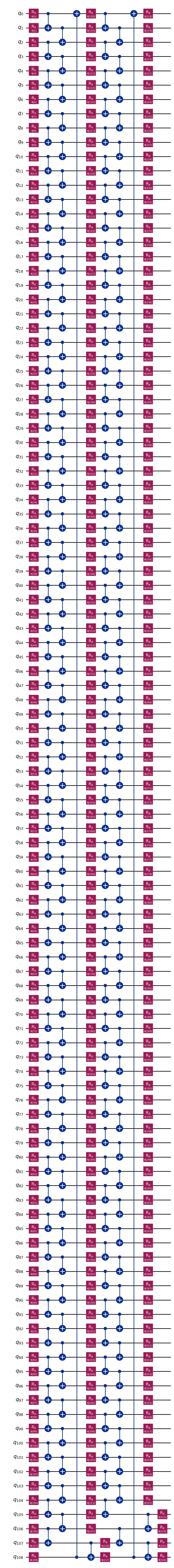
ansatz.draw("mpl", fold=-1)

เพื่อตรวจสอบคุณภาพของผลลัพธ์ที่ได้จาก circuit cutting เราจำเป็นต้องรู้ผลลัพธ์ที่เหมาะสมที่สุด Circuit ที่เลือกในปัจจุบันนั้นเกินกว่าการจำลอง classical แบบ brute force ดังนั้น เราจึงกำหนดค่าพารามิเตอร์ให้กับ Circuit อย่างระมัดระวังเพื่อทำให้เป็น Clifford

เราจะกำหนดค่าพารามิเตอร์เป็น $0$ สำหรับสองเลเยอร์แรกของ Rx gate และค่า $\pi$ สำหรับเลเยอร์สุดท้าย ซึ่งทำให้ผลลัพธ์ที่เหมาะสมของ Circuit นี้คือ $|1\rangle^{\otimes n}$ โดย $n$ คือจำนวน Qubit ดังนั้น expectation values ของ $\langle Z_i \rangle$ และ $\langle Z_i Z_{i+1} \rangle$ ซึ่ง $i$ คือดัชนีของ Qubit จะมีค่าเป็น $-1$ และ $+1$ ตามลำดับ

params_last_layer = [np.pi] * ansatz.num_qubits
params = [0] * (ansatz.num_parameters - ansatz.num_qubits)
params.extend(params_last_layer)

ansatz.assign_parameters(params, inplace=True)

เลือก observable

เพื่อวัดประโยชน์ของ gate cutting เราวัด expectation values ของ observable $\frac{1}{n}\sum_{i=1}^n \langle Z_i \rangle$ และ $\frac{1}{n-1}\sum_{i=1}^{n-1} \langle Z_i Z_{i+1} \rangle$ ตามที่กล่าวถึงก่อนหน้านี้ expectation values ที่เหมาะสมคือ $-1$ และ $+1$ ตามลำดับ

observables = []

for i in range(num_qubits):
    obs = "I" * (i) + "Z" + "I" * (num_qubits - i - 1)
    observables.append(obs)

for i in range(num_qubits):
    if i == num_qubits - 1:
        obs = "Z" + "I" * (num_qubits - 2) + "Z"
    else:
        obs = "I" * i + "ZZ" + "I" * (num_qubits - i - 2)
    observables.append(obs)

observables = SparsePauliOp(observables)
paulis = observables.paulis
coeffs = observables.coeffs

ขั้นตอนที่ 2: ปรับปัญหาให้เหมาะสมสำหรับการรันบน quantum hardware

• อินพุต: Abstract circuit และ observable
• เอาต์พุต: Target circuit และ observable ที่ผลิตโดยการตัด gate ระยะไกล

Transpile Circuit

โปรดสังเกตว่า Circuit สามารถถูก transpile ในขั้นตอนนี้ หรือหลังจากการตัดก็ได้ ถ้าเรา transpile หลังจากการตัด จะต้อง transpile แต่ละ subexperiment ที่เกิดจาก sampling overhead ดังนั้นจึงควรทำการ transpile ในขั้นตอนนี้มากกว่าเพื่อลด overhead ของการ transpilation

อย่างไรก็ตาม ถ้าทำการ transpilation ในขั้นตอนนี้ด้วย native hardware connectivity Transpiler จะเพิ่ม SWAP gate หลายตัวเพื่อจัด periodic 2-qubit operation ซึ่งจะทำให้ประโยชน์ของ circuit cutting ไม่ชัดเจน เพื่อหลีกเลี่ยงปัญหานี้ เราสามารถใช้ประโยชน์จากการที่เรารู้ gate ที่ต้องตัดอย่างแน่ชัด โดยเฉพาะอย่างยิ่ง เราสามารถสร้าง virtual coupling map โดยเพิ่ม virtual connection ระหว่าง Qubit ที่อยู่ห่างกันเพื่อรองรับ periodic 2-qubit gate เหล่านี้ ซึ่งจะทำให้ Circuit สามารถถูก transpile ในขั้นตอนนี้โดยไม่ต้องใช้ SWAP gate ส่วนเกิน

coupling_map = backend.configuration().coupling_map

# create a virtual coupling map with long range connectivity
virtual_coupling_map = coupling_map.copy()
virtual_coupling_map.append([init_layout[-1], init_layout[0]])
virtual_coupling_map.append([init_layout[0], init_layout[-1]])

pm_virtual = generate_preset_pass_manager(
    optimization_level=1,
    coupling_map=virtual_coupling_map,
    initial_layout=init_layout,
    basis_gates=backend.configuration().basis_gates,
)

virtual_mapped_circuit = pm_virtual.run(ansatz)
virtual_mapped_circuit.draw("mpl", fold=-1, idle_wires=False)

ตัด periodic connectivity ระยะไกล

ตอนนี้เราจะตัด gate ใน Circuit ที่ถูก transpile แล้ว โปรดสังเกตว่า 2-qubit gate ที่ต้องตัดคือ gate ที่เชื่อม Qubit สุดท้ายและ Qubit แรกของ layout

# Find the indices of the distant gates
cut_indices = [
    i
    for i, instruction in enumerate(virtual_mapped_circuit.data)
    if {virtual_mapped_circuit.find_bit(q)[0] for q in instruction.qubits}
    == {init_layout[-1], init_layout[0]}
]

เราจะนำ layout ของ Circuit ที่ถูก transpile แล้วไปใช้กับ observable

trans_observables = observables.apply_layout(virtual_mapped_circuit.layout)

สุดท้าย subexperiment จะถูกสร้างขึ้นโดยการ sample จาก measurement และ preparation basis ที่แตกต่างกัน

qpd_circuit, bases = cut_gates(virtual_mapped_circuit, cut_indices)
subexperiments, coefficients = generate_cutting_experiments(
    circuits=qpd_circuit,
    observables=trans_observables.paulis,
    num_samples=np.inf,
)

โปรดสังเกตว่าการตัด long-range interaction นำไปสู่การรัน sample ของ Circuit หลายตัวที่ต่างกันในด้าน measurement และ preparation basis ข้อมูลเพิ่มเติมเกี่ยวกับเรื่องนี้สามารถหาได้ใน Constructing a virtual two-qubit gate by sampling single-qubit operations และ Cutting circuits with multiple two-qubit unitaries

จำนวน periodic gate ที่ต้องตัดจะเท่ากับจำนวนครั้งที่ทำซ้ำของเลเยอร์ TwoLocal ที่กำหนดเป็น num_reps ข้างต้น sampling overhead ของ gate cutting คือ 6 ดังนั้น จำนวน subexperiment ทั้งหมดจะเป็น $6^{num\_reps}$

print(f"Number of subexperiments is {len(subexperiments)} = 6**{num_reps}")

Number of subexperiments is 36 = 6**2

Transpile subexperiment

ณ จุดนี้ subexperiment ประกอบด้วย Circuit ที่มี 1-qubit gate บางตัวที่ไม่อยู่ใน basis gate set ซึ่งเป็นเพราะ Qubit ที่ถูกตัดถูกวัดใน basis ที่แตกต่างกัน และ rotation gate ที่ใช้สำหรับสิ่งนี้ไม่จำเป็นต้องอยู่ใน basis gate set ตัวอย่างเช่น การวัดใน X basis หมายถึงการใช้ Hadamard gate ก่อนการวัดปกติใน Z basis แต่ Hadamard ไม่ได้เป็นส่วนหนึ่งของ basis gate set

แทนที่จะใช้กระบวนการ transpilation ทั้งหมดกับแต่ละ Circuit ใน subexperiment เราสามารถใช้ transpilation pass เฉพาะแทนได้ ดูรายละเอียดเพิ่มเติมของ transpilation pass ทั้งหมดที่มีได้ที่ เอกสารนี้

เราจะใช้ pass BasisTranslator จากนั้น Optimize1qGatesDecomposition เพื่อให้แน่ใจว่า gate ทั้งหมดใน Circuit เหล่านี้อยู่ใน basis gate set การใช้สอง pass นี้เร็วกว่ากระบวนการ transpilation ทั้งหมด เนื่องจากขั้นตอนอื่นๆ เช่น routing และการเลือก initial layout จะไม่ถูกดำเนินการอีกครั้ง

pass_ = PassManager(
    [Optimize1qGatesDecomposition(basis=backend.configuration().basis_gates)]
)

subexperiments = pass_.run(
    [
        dag_to_circuit(
            BasisTranslator(sel, target_basis=backend.basis_gates).run(
                circuit_to_dag(circ)
            )
        )
        for circ in subexperiments
    ]
)

ขั้นตอนที่ 3: รันด้วย Qiskit primitives

• Input: Target circuits
• Output: การกระจาย quasi-probability

เราใช้ primitive SamplerV2 สำหรับการรัน cut circuits เราปิดการใช้งาน dynamical decoupling และ twirling เพื่อให้ผลลัพธ์ที่ดีขึ้นเกิดจากการใช้ gate cutting อย่างมีประสิทธิภาพสำหรับ circuit ประเภทนี้เพียงอย่างเดียว

options = SamplerOptions()
options.default_shots = 10000
options.dynamical_decoupling.enable = False
options.twirling.enable_gates = False
options.twirling.enable_measure = False

ตอนนี้เราจะส่ง job โดยใช้ batch mode

with Batch(backend=backend) as batch:
    sampler = SamplerV2(options=options)
    cut_job = sampler.run(subexperiments)

print(f"Job ID {cut_job.job_id()}")

Job ID cwxf7wq60bqg008pvt8g

result = cut_job.result()

ขั้นตอนที่ 4: Post-process และแสดงผลลัพธ์ในรูปแบบ classical ที่ต้องการ

• Input: การกระจาย quasi-probability
• Output: ค่า expectation ที่ถูก reconstruct แล้ว

reconstructed_expvals = reconstruct_expectation_values(
    result,
    coefficients,
    paulis,
)

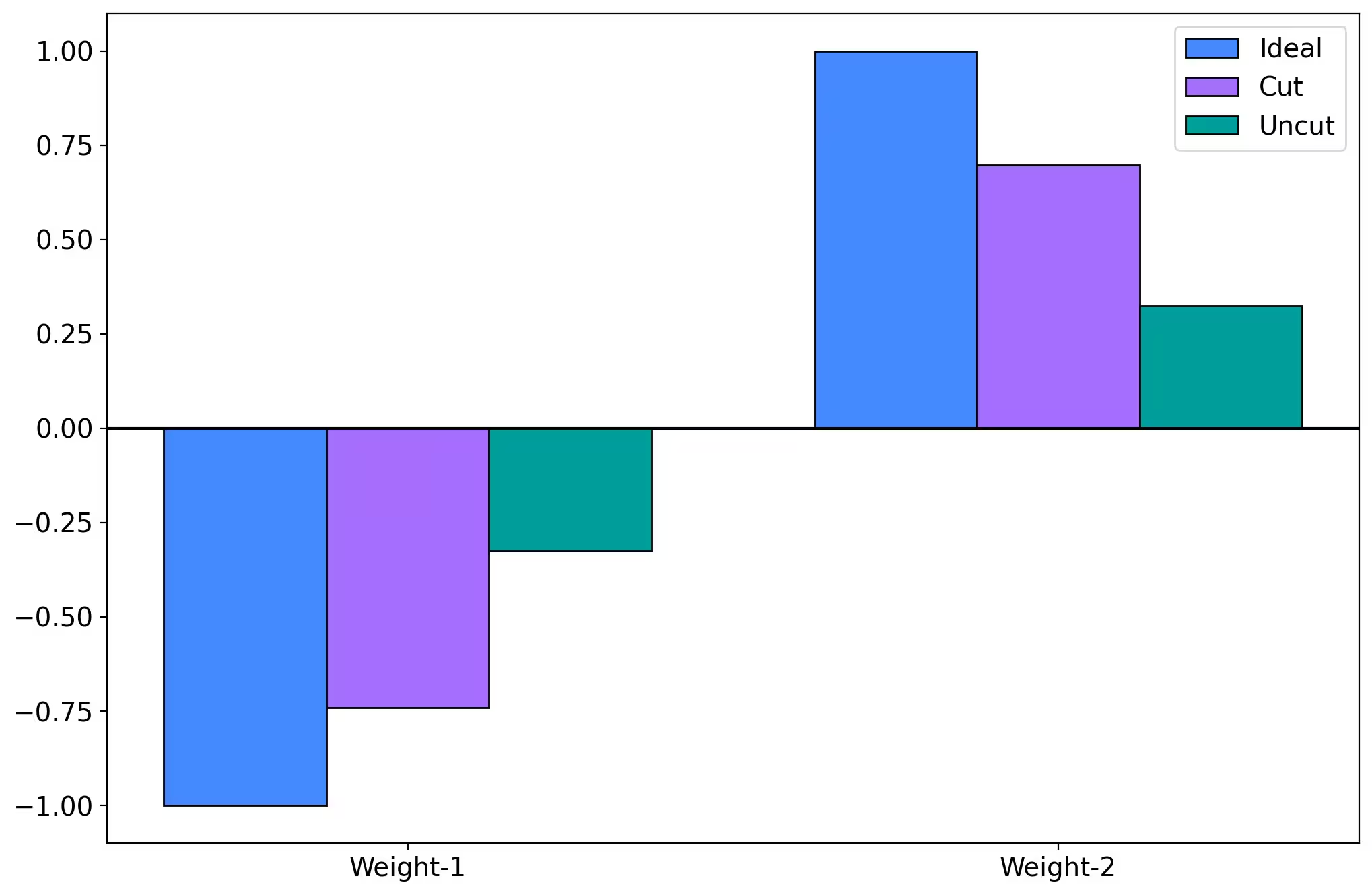
ตอนนี้เราจะคำนวณค่าเฉลี่ยของ Z-type observables น้ำหนัก 1 และน้ำหนัก 2

cut_weight_1 = np.mean(reconstructed_expvals[:num_qubits])
cut_weight_2 = np.mean(reconstructed_expvals[num_qubits:])

print(f"Average of weight-1 expectation values is {cut_weight_1}")
print(f"Average of weight-2 expectation values is {cut_weight_2}")

Average of weight-1 expectation values is -0.741733944954063
Average of weight-2 expectation values is 0.6968862385320495

Cross Verify: รับค่า expectation แบบไม่ตัด

การ cross-verify ข้อได้เปรียบของเทคนิค circuit cutting เทียบกับแบบไม่ตัดนั้นมีประโยชน์มาก ที่นี่เราจะคำนวณค่า expectation โดยไม่ตัด circuit โปรดทราบว่า circuit แบบไม่ตัดจะประสบปัญหาจาก SWAP gate จำนวนมากที่จำเป็นสำหรับการดำเนินการ 2-qubit ระหว่าง qubit แรกและ qubit สุดท้าย เราจะใช้ฟังก์ชัน sampled_expectation_value เพื่อรับค่า expectation ของ circuit แบบไม่ตัดหลังจากได้รับการกระจายความน่าจะเป็นผ่าน SamplerV2 ซึ่งช่วยให้ใช้ primitive อย่างสม่ำเสมอในทุกกรณี อย่างไรก็ตาม โปรดทราบว่าเราสามารถใช้ EstimatorV2 เพื่อคำนวณค่า expectation โดยตรงได้เช่นกัน

if ansatz.num_clbits == 0:
    ansatz.measure_all()

pm_uncut = generate_preset_pass_manager(
    optimization_level=1, backend=backend, initial_layout=init_layout
)

transpiled_circuit = pm_uncut.run(ansatz)

sampler = SamplerV2(mode=backend, options=options)
uncut_job = sampler.run([transpiled_circuit])

uncut_job_id = uncut_job.job_id()
print(f"The job id for the uncut clifford circuit is {uncut_job_id}")

The job id for the uncut clifford circuit is cwxfads2ac5g008jhe7g

uncut_result = uncut_job.result()[0]
uncut_counts = uncut_result.data.meas.get_counts()

ตอนนี้เราจะคำนวณค่าเฉลี่ย expectation ของ Z-type observables น้ำหนัก 1 และน้ำหนัก 2 ทั้งหมดโดยไม่ตัด

uncut_expvals = [
    sampled_expectation_value(uncut_counts, obs) for obs in paulis
]

uncut_weight_1 = np.mean(uncut_expvals[:num_qubits])
uncut_weight_2 = np.mean(uncut_expvals[num_qubits:])

print(f"Average of weight-1 expectation values is {uncut_weight_1}")
print(f"Average of weight-2 expectation values is {uncut_weight_2}")

Average of weight-1 expectation values is -0.32494128440366965
Average of weight-2 expectation values is 0.32340917431192656

Visualize

ตอนนี้เราจะแสดงภาพการปรับปรุงที่ได้สำหรับ observables น้ำหนัก 1 และน้ำหนัก 2 เมื่อใช้ gate cutting สำหรับ periodic chain circuit

mpl.rcParams.update(mpl.rcParamsDefault)

fig = plt.subplots(figsize=(12, 8), dpi=200)
width = 0.25
labels = ["Weight-1", "Weight-2"]
x = np.arange(len(labels))

ideal = [-1, 1]
cut = [cut_weight_1, cut_weight_2]
uncut = [uncut_weight_1, uncut_weight_2]

br1 = np.arange(len(ideal))
br2 = [x + width for x in br1]
br3 = [x + width for x in br2]

plt.bar(
    br1, ideal, width=width, edgecolor="k", label="Ideal", color="#4589ff"
)
plt.bar(br2, cut, width=width, edgecolor="k", label="Cut", color="#a56eff")
plt.bar(
    br3, uncut, width=width, edgecolor="k", label="Uncut", color="#009d9a"
)

plt.axhline(y=0, color="k", linestyle="-")

plt.xticks([r + width for r in range(len(ideal))], labels, fontsize=14)
plt.yticks(fontsize=14)

plt.legend(fontsize=14)
plt.show()

สรุป

โดยสรุป เราคำนวณค่าเฉลี่ย expectation ของ Z-type observables น้ำหนัก 1 และน้ำหนัก 2 สำหรับ periodic 1D chain ของ 109 qubits เพื่อให้บรรลุเป้าหมายนี้ เรา

• สร้าง virtual coupling map โดยเพิ่ม connectivity ระยะไกลระหว่าง qubit แรกและ qubit สุดท้ายของ 1D chain และ transpile circuit
  • การ transpile ในขั้นตอนนี้ช่วยให้เราหลีกเลี่ยงค่าใช้จ่ายในการ transpile แต่ละ subexperiment แยกกันหลังจากตัด
  • การใช้ virtual coupling map ช่วยให้เราหลีกเลี่ยง SWAP gate พิเศษสำหรับการดำเนินการ 2-qubit ระหว่าง qubit แรกและ qubit สุดท้าย
• ลบ connectivity ระยะไกลออกจาก circuit ที่ transpile แล้วด้วย gate cutting
• แปลง cut circuits เป็น basis gate set โดยใช้ transpilation passes ที่เหมาะสม
• รัน cut circuits บนอุปกรณ์ IBM Quantum โดยใช้ primitive SamplerV2
• ได้รับค่า expectation โดย reconstruct ผลลัพธ์ของ cut circuits

ข้อสรุป

เราสังเกตจากผลลัพธ์ว่าค่าเฉลี่ยของ observables ประเภท $\langle Z \rangle$ น้ำหนัก 1 และ $\langle ZZ \rangle$ น้ำหนัก 2 ดีขึ้นอย่างมีนัยสำคัญจากการตัด periodic gates โปรดทราบว่าการศึกษานี้ไม่รวมเทคนิคการระงับหรือลดความผิดพลาด การปรับปรุงที่สังเกตได้เกิดจากการใช้ gate cutting อย่างถูกต้องสำหรับปัญหานี้เพียงอย่างเดียว ผลลัพธ์สามารถปรับปรุงได้มากขึ้นโดยใช้เทคนิคการลดและระงับความผิดพลาด

การศึกษานี้แสดงตัวอย่างการใช้ gate cutting อย่างมีประสิทธิภาพเพื่อปรับปรุงประสิทธิภาพของการคำนวณ

แบบสำรวจ Tutorial

Link to survey

Note: This survey is provided by IBM Quantum and relates to the original English content. To give feedback on doQumentation's website, translations, or code execution, please open a GitHub issue.

กรุณาทำแบบสำรวจสั้นนี้เพื่อให้ feedback เกี่ยวกับ tutorial นี้ ข้อมูลของคุณจะช่วยให้เราปรับปรุงเนื้อหาและประสบการณ์การใช้งาน