การคอมไพล์วงจรควอนตัมแบบประมาณสำหรับการวิวัฒน์ตามเวลา

ประมาณการการใช้งาน: 15 วินาทีบนโปรเซสเซอร์ Heron (หมายเหตุ: นี่เป็นเพียงการประมาณการ ระยะเวลาจริงอาจแตกต่างกัน)

ผลการเรียนรู้

หลังจากทำบทช่วยสอนนี้เสร็จสิ้น คุณจะเข้าใจข้อมูลต่อไปนี้:

วิธีใช้ AQC-Tensor Qiskit addon เพื่อบีบอัด Trotter circuit ที่ลึกให้เป็น ansatz circuit ที่ตื้นกว่า
วิธีสร้าง parametrized ansatz จาก Trotter circuit และปรับแต่งพารามิเตอร์โดยใช้วิธี tensor network (MPS)
วิธีประเมิน fidelity ของวงจรที่บีบอัดแล้วเทียบกับ target evolution และรันบนฮาร์ดแวร์ควอนตัม

สิ่งที่ควรรู้ก่อน

แนะนำให้ศึกษาหัวข้อเหล่านี้ก่อน:

ภูมิหลัง

บทช่วยสอนนี้สาธิตวิธีการใช้งาน Approximate Quantum Compilation โดยใช้ tensor network (AQC-Tensor) กับ Qiskit เพื่อเพิ่มประสิทธิภาพของวงจรควอนตัม AQC-Tensor บีบอัด Trotter circuit ที่ลึกให้เป็นวงจรที่ตื้นกว่าและเหมาะกับฮาร์ดแวร์มากขึ้น โดยรักษาความแม่นยำของการจำลองไว้

AQC-Tensor ทำงานอย่างไร

สมมติว่าต้องการจำลอง Hamiltonian $H$ ตลอดเวลารวม $t$ โดยใช้ $k$ Trotter steps วงจร Trotter แบบเต็มคือ:

U_{\text{full}} = \left[U_{\text{Trotter}}(t/k)\right]^k

วิธีง่ายๆ ใช้ Trotter step น้อยเพื่อรักษาความลึกของวงจรให้จัดการได้ แต่จะเกิด Trotter error มาก AQC-Tensor แก้ปัญหานี้โดยแยกความแม่นยำออกจากความลึก:

Target circuit (ความแม่นยำสูง ลึก): สร้าง Trotter circuit ที่มีหลาย step ประมาณ $10k$ สำหรับเวลาวิวัฒนาการเดิม circuit นี้มี Trotter error น้อยกว่ามาก แต่ลึกเกินไปสำหรับฮาร์ดแวร์ เนื่องจากจำลองแบบคลาสสิกในรูป matrix product state (MPS) ความลึกจึงไม่ใช่ปัญหา
Ansatz circuit (ความลึกต่ำ มีพารามิเตอร์): กำหนด parametrized circuit $V(\theta)$ ที่มีโครงสร้างเดียวกับ Trotter circuit แบบ single-step กำหนดค่าเริ่มต้นให้ $V(\theta_{\text{init}}) = U_{\text{Trotter}}(t/k)$ จากนั้นปรับ $\theta$ ซ้ำๆ เพื่อให้ $V(\theta)$ ให้ผลลัพธ์ของ target state ที่มีความแม่นยำสูงได้ใกล้เคียงที่สุด

ผลลัพธ์คือวงจรที่รักษาความลึกของ Trotter step เดียว แต่ได้ความแม่นยำเทียบเท่ากับหลาย step ทำให้เหมาะกับฮาร์ดแวร์ควอนตัมในยุคใกล้

เมื่อไหรที่ควรใช้ AQC-Tensor

AQC-Tensor มีประสิทธิภาพสูงสุดเมื่อ:

ความลึกของวงจรเกิน coherence time ของฮาร์ดแวร์ หาก Trotter simulation ต้องการ Trotter step มากกว่าที่ device รองรับ AQC-Tensor สามารถบีบอัด evolution ให้เป็นวงจรที่ตื้นกว่าได้
Entanglement ยังจัดการได้แบบคลาสสิก entanglement รวมในสถานะที่วิวัฒน์ตามเวลาขึ้นกับเวลา $t$ เป็นหลัก ไม่ใช่จำนวน Trotter step $k$ ซึ่งหมายความว่า target circuit ที่มี $10k$ step มักไม่ยากกว่าในการแสดงเป็น MPS มากกว่า circuit ที่มี $k$ step ตราบใดที่ $t$ สั้นพอที่ bond dimension ยังจัดการได้
มี ansatz ที่เป็นธรรมชาติ เนื่องจาก ansatz สะท้อนโครงสร้างของ Trotter circuit จึงมีจุดเริ่มต้นที่มีแรงจูงใจทางฟิสิกส์พร้อมพารามิเตอร์เริ่มต้นที่กำหนดชัดเจน ช่วยหลีกเลี่ยงปัญหาการ convergence ที่มักเกิดกับ variational ansatze แบบทั่วไป

วิธีนี้แตกต่างจากการบีบอัดวงจรทั่วไป แทนที่จะพยายามประมาณ unitary ที่กำหนดเองด้วย gate น้อยลง AQC-Tensor คงโครงสร้าง gate เดิมและปรับพารามิเตอร์เพื่อลด Trotter error ดูรายละเอียดเพิ่มเติมได้ใน AQC-Tensor documentation

บทช่วยสอนนี้นำทางคุณผ่าน AQC-Tensor workflow แบบ full state-preparation: กำหนด Hamiltonian สร้าง Trotter circuit บีบอัดด้วยการปรับแต่ง tensor-network และรันผลลัพธ์บนฮาร์ดแวร์ IBM Quantum®

ข้อกำหนดเบื้องต้น

ก่อนเริ่มบทช่วยสอนนี้ ตรวจสอบให้แน่ใจว่าคุณได้ติดตั้งสิ่งต่อไปนี้:

Qiskit SDK v2.0 หรือใหม่กว่า พร้อมรองรับ visualization
Qiskit Runtime v0.22 หรือใหม่กว่า (pip install qiskit-ibm-runtime)
AQC-Tensor Qiskit addon (pip install 'qiskit-addon-aqc-tensor[aer,quimb-jax]')

การตั้งค่า

# Added by doQumentation — required packages for this notebook
!pip install -q matplotlib numpy qiskit qiskit-addon-aqc-tensor qiskit-addon-utils qiskit-ibm-runtime quimb rustworkx scipy

import numpy as np
import quimb.tensor
import datetime
import matplotlib.pyplot as plt

from scipy.linalg import expm
from scipy.optimize import OptimizeResult, minimize

from qiskit.quantum_info import SparsePauliOp, Pauli
from qiskit.transpiler import CouplingMap
from qiskit.transpiler.preset_passmanagers import generate_preset_pass_manager
from qiskit import QuantumCircuit
from qiskit.synthesis import SuzukiTrotter

from qiskit_addon_utils.problem_generators import (
    generate_time_evolution_circuit,
)
from qiskit_addon_aqc_tensor.ansatz_generation import (
    generate_ansatz_from_circuit,
)
from qiskit_addon_aqc_tensor.objective import MaximizeStateFidelity
from qiskit_addon_aqc_tensor.simulation.quimb import QuimbSimulator
from qiskit_addon_aqc_tensor.simulation import tensornetwork_from_circuit
from qiskit_addon_aqc_tensor.simulation import compute_overlap

from qiskit_ibm_runtime import QiskitRuntimeService
from qiskit_ibm_runtime import EstimatorV2 as Estimator
from qiskit_ibm_runtime.fake_provider import FakeKyiv

from rustworkx.visualization import graphviz_draw

ตัวอย่างขนาดเล็กด้วย simulator

ส่วนนี้ใช้ระบบ 10 ไซต์เพื่ออธิบาย AQC-Tensor workflow ทีละขั้นตอน เราจำลองพลวัตของ XXZ spin chain ขนาด 10 ไซต์ ซึ่งเป็นโมเดลที่ได้รับการศึกษาอย่างแพร่หลายสำหรับการตรวจสอบปฏิสัมพันธ์ spin และคุณสมบัติทางแม่เหล็ก

Hamiltonian คือ:

\hat{\mathcal{H}}_{XXZ} = \sum_{i=1}^{L-1} J_{i,(i+1)}\left(X_i X_{(i+1)}+Y_i Y_{(i+1)}+ 2\cdot Z_i Z_{(i+1)} \right) \, ,

โดยที่ $J_{i,(i+1)}$ คือสัมประสิทธิ์แบบสุ่มสำหรับเส้น $(i, i+1)$ และ $L=10$

ขั้นตอนที่ 1: แมป input แบบคลาสสิกไปยังปัญหาควอนตัม

ในขั้นตอนนี้ เราจะ:

กำหนด Hamiltonian, observable และสถานะเริ่มต้น
คำนวณค่า expectation value ที่แม่นยำแบบคลาสสิกสำหรับการเปรียบเทียบในภายหลัง
สร้าง Trotter circuit ที่มีความแม่นยำสูง (AQC target) และบีบอัดให้เป็น ansatz ที่มีความลึกต่ำโดยใช้ AQC-Tensor

ตั้งค่า Hamiltonian, observable และสถานะเริ่มต้น

# L is the number of sites in the 1D spin chain
L = 10

# Generate the coupling map
edge_list = [(i - 1, i) for i in range(1, L)]
even_edges = edge_list[::2]
odd_edges = edge_list[1::2]
coupling_map = CouplingMap(edge_list)

# Generate random coefficients for our XXZ Hamiltonian
np.random.seed(0)
Js = np.random.rand(L - 1) + 0.5 * np.ones(L - 1)
hamiltonian = SparsePauliOp(Pauli("I" * L))
for i, edge in enumerate(even_edges + odd_edges):
    hamiltonian += SparsePauliOp.from_sparse_list(
        [
            ("XX", (edge), Js[i] / 2),
            ("YY", (edge), Js[i] / 2),
            ("ZZ", (edge), Js[i]),
        ],
        num_qubits=L,
    )

# Generate a ZZ observable between the two middle qubits
observable = SparsePauliOp.from_sparse_list(
    [("ZZ", (L // 2 - 1, L // 2), 1.0)], num_qubits=L
)

# Generate an initial Néel state |1010101010⟩
initial_state_circuit = QuantumCircuit(L)
for i in range(L):
    if i % 2:
        initial_state_circuit.x(i)

print("Hamiltonian:", hamiltonian)
print("Observable:", observable)
graphviz_draw(coupling_map.graph, method="circo")

Hamiltonian: SparsePauliOp(['IIIIIIIIII', 'IIIIIIIIXX', 'IIIIIIIIYY', 'IIIIIIIIZZ', 'IIIIIIXXII', 'IIIIIIYYII', 'IIIIIIZZII', 'IIIIXXIIII', 'IIIIYYIIII', 'IIIIZZIIII', 'IIXXIIIIII', 'IIYYIIIIII', 'IIZZIIIIII', 'XXIIIIIIII', 'YYIIIIIIII', 'ZZIIIIIIII', 'IIIIIIIXXI', 'IIIIIIIYYI', 'IIIIIIIZZI', 'IIIIIXXIII', 'IIIIIYYIII', 'IIIIIZZIII', 'IIIXXIIIII', 'IIIYYIIIII', 'IIIZZIIIII', 'IXXIIIIIII', 'IYYIIIIIII', 'IZZIIIIIII'],
              coeffs=[1.        +0.j, 0.52440675+0.j, 0.52440675+0.j, 1.0488135 +0.j,
 0.60759468+0.j, 0.60759468+0.j, 1.21518937+0.j, 0.55138169+0.j,
 0.55138169+0.j, 1.10276338+0.j, 0.52244159+0.j, 0.52244159+0.j,
 1.04488318+0.j, 0.4618274 +0.j, 0.4618274 +0.j, 0.9236548 +0.j,
 0.57294706+0.j, 0.57294706+0.j, 1.14589411+0.j, 0.46879361+0.j,
 0.46879361+0.j, 0.93758721+0.j, 0.6958865 +0.j, 0.6958865 +0.j,
 1.391773  +0.j, 0.73183138+0.j, 0.73183138+0.j, 1.46366276+0.j])
Observable: SparsePauliOp(['IIIIZZIIII'],
              coeffs=[1.+0.j])

Output of the previous code cell

คำนวณค่า expectation value ที่แม่นยำ

สำหรับระบบขนาดนี้ เราสามารถคำนวณค่า expectation value ที่วิวัฒน์ตามเวลาแบบแม่นยำได้โดยตรงโดยใช้การ exponentiation matrix ซึ่งเป็น ground truth สำหรับการประเมินความแม่นยำของ AQC circuit

aqc_evolution_time = 0.2

# Each baseline Trotter step covers dt = aqc_evolution_time / 3
# The subsequent (uncompressed) step covers 1 additional dt
subsequent_evolution_time = aqc_evolution_time / 3
total_evolution_time = aqc_evolution_time + subsequent_evolution_time

# Compute exact expectation value via matrix exponentiation
H_matrix = hamiltonian.to_matrix()
U_exact = expm(-1j * H_matrix * total_evolution_time)

# Build the initial state vector (Néel state)
initial_state_vec = np.zeros(2**L)
state_idx = sum(2**i for i in range(L) if i % 2)
initial_state_vec[state_idx] = 1.0

# Evolve and compute expectation value
evolved_state = U_exact @ initial_state_vec
obs_matrix = observable.to_matrix()
exact_expval = (evolved_state.conj() @ obs_matrix @ evolved_state).real

print(f"AQC evolution time: {aqc_evolution_time}")
print(f"Subsequent evolution time: {subsequent_evolution_time:.6f}")
print(f"Total evolution time: {total_evolution_time:.6f}")
print(f"Exact expectation value: {exact_expval:.6f}")

AQC evolution time: 0.2
Subsequent evolution time: 0.066667
Total evolution time: 0.266667
Exact expectation value: -0.700899

สร้าง AQC target circuit

ตอนนี้เราสร้าง Trotter circuit ที่จะเป็น AQC target circuit นี้ใช้ Trotter step จำนวนมาก (32) เพื่อความแม่นยำสูง เนื่องจากจะถูกจำลองแบบคลาสสิกในรูป MPS เท่านั้น ไม่ใช่รันบนฮาร์ดแวร์ ความลึกมากจึงไม่ใช่ปัญหา

aqc_target_num_trotter_steps = 32

aqc_target_circuit = initial_state_circuit.copy()
aqc_target_circuit.compose(
    generate_time_evolution_circuit(
        hamiltonian,
        synthesis=SuzukiTrotter(reps=aqc_target_num_trotter_steps),
        time=aqc_evolution_time,
    ),
    inplace=True,
)

สร้าง ansatz, พารามิเตอร์เริ่มต้น, subsequent circuit และ baseline circuit

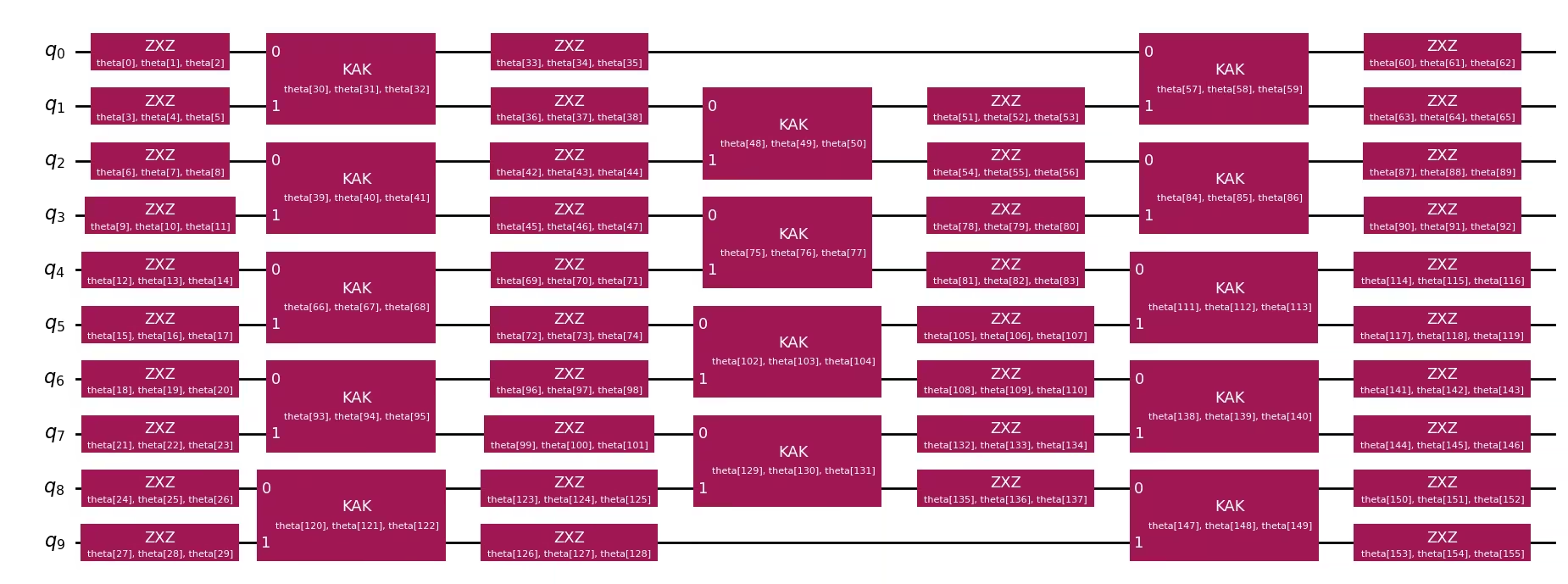
ต่อไป เราสร้างวงจร "good" ที่มีเวลาวิวัฒนาการเดียวกับ AQC target แต่มี Trotter step น้อยกว่ามาก (แค่หนึ่ง step) เราส่งวงจรนี้ไปยัง generate_ansatz_from_circuit ซึ่งส่งคืน:

วงจร ansatz ที่มีพารามิเตอร์ทั่วไปพร้อมการเชื่อมต่อ two-qubit เดียวกัน
พารามิเตอร์เริ่มต้น ที่ให้ผลลัพธ์เป็นวงจร input เมื่อใส่เข้าไปใน ansatz

นอกจากนี้เรายังสร้าง:

subsequent circuit ที่มี Trotter step เดียวที่จะต่อท้าย (ไม่บีบอัด) หลังส่วนที่ปรับด้วย AQC ตามแนวทางใน AQC-Tensor initial state tutorial
baseline Trotter circuit ที่ใช้ Trotter step สี่ step ตลอดเวลาวิวัฒนาการทั้งหมด (aqc_evolution_time + subsequent_evolution_time) ใช้เป็นการเปรียบเทียบ: แสดงสิ่งที่จะรันบนฮาร์ดแวร์โดยไม่ใช้ AQC AQC ansatz (3 step บีบอัด + 1 step ไม่บีบอัด) ให้ความแม่นยำที่ดีกว่าที่ความลึกต่ำกว่า

aqc_ansatz_num_trotter_steps = 1

aqc_good_circuit = initial_state_circuit.copy()
aqc_good_circuit.compose(
    generate_time_evolution_circuit(
        hamiltonian,
        synthesis=SuzukiTrotter(reps=aqc_ansatz_num_trotter_steps),
        time=aqc_evolution_time,
    ),
    inplace=True,
)

aqc_ansatz, aqc_initial_parameters = generate_ansatz_from_circuit(
    aqc_good_circuit
)

# Subsequent circuit: 1 non-compressed Trotter step appended after AQC
subsequent_num_trotter_steps = 1
subsequent_circuit = generate_time_evolution_circuit(
    hamiltonian,
    synthesis=SuzukiTrotter(reps=subsequent_num_trotter_steps),
    time=subsequent_evolution_time,
)

# Baseline Trotter circuit: 4 Trotter steps over total evolution time, no AQC
baseline_num_trotter_steps = 4
baseline_circuit = initial_state_circuit.copy()
baseline_circuit.compose(
    generate_time_evolution_circuit(
        hamiltonian,
        synthesis=SuzukiTrotter(reps=baseline_num_trotter_steps),
        time=total_evolution_time,
    ),
    inplace=True,
)

print(
    f"Target circuit:      depth {aqc_target_circuit.depth(lambda x: x.operation.num_qubits == 2)}"
)
print(
    f"Baseline circuit:    depth {baseline_circuit.depth(lambda x: x.operation.num_qubits == 2)} ({baseline_num_trotter_steps} Trotter steps, time={total_evolution_time:.4f})"
)
print(
    f"Subsequent circuit:  depth {subsequent_circuit.depth(lambda x: x.operation.num_qubits == 2)} ({subsequent_num_trotter_steps} Trotter step, time={subsequent_evolution_time:.4f})"
)
print(
    f"Ansatz circuit:      depth {aqc_ansatz.depth(lambda x: x.operation.num_qubits == 2)}, with {len(aqc_initial_parameters)} parameters"
)
aqc_ansatz.draw("mpl", fold=-1)

Target circuit:      depth 384
Baseline circuit:    depth 48 (4 Trotter steps, time=0.2667)
Subsequent circuit:  depth 12 (1 Trotter step, time=0.0667)
Ansatz circuit:      depth 3, with 156 parameters

Output of the previous code cell

ตั้งค่าการจำลอง tensor network และสร้าง target MPS

เราใช้ quimb matrix-product state (MPS) circuit simulator โดยมี JAX ให้ gradient อัตโนมัติสำหรับการปรับแต่งแบบ gradient-based จากนั้นเราสร้างการแสดง MPS ของ target state และประเมิน starting fidelity ระหว่าง initial ansatz กับ target เนื่องจากปัญหานี้เป็นตัวอย่างขนาดค่อนข้างเล็ก starting fidelity จึงค่อนข้างสูง

simulator_settings = QuimbSimulator(
    quimb.tensor.CircuitMPS, autodiff_backend="jax"
)

aqc_target_mps = tensornetwork_from_circuit(
    aqc_target_circuit, simulator_settings
)
print("Target MPS maximum bond dimension:", aqc_target_mps.psi.max_bond())

good_mps = tensornetwork_from_circuit(aqc_good_circuit, simulator_settings)
starting_fidelity = abs(compute_overlap(good_mps, aqc_target_mps)) ** 2
print(f"Starting fidelity: {starting_fidelity:.6f}")

Target MPS maximum bond dimension: 5
Starting fidelity: 0.998246

ปรับแต่งพารามิเตอร์ ansatz

เราใช้ L-BFGS-B optimizer เพื่อย่อ cost function MaximizeStateFidelity optimizer ปรับพารามิเตอร์ ansatz ซ้ำๆ เพื่อเพิ่ม fidelity ระหว่าง ansatz circuit กับ target MPS

aqc_stopping_fidelity = 1
aqc_max_iterations = 500

stopping_point = 1.0 - aqc_stopping_fidelity
objective = MaximizeStateFidelity(
    aqc_target_mps, aqc_ansatz, simulator_settings
)

def callback(intermediate_result: OptimizeResult):
    fidelity = 1 - intermediate_result.fun
    print(
        f"{datetime.datetime.now()} Intermediate result: Fidelity {fidelity:.8f}"
    )
    if intermediate_result.fun < stopping_point:
        raise StopIteration

result = minimize(
    objective,
    aqc_initial_parameters,
    method="L-BFGS-B",
    jac=True,
    options={"maxiter": aqc_max_iterations},
    callback=callback,
)
if result.status not in (0, 1, 99):
    raise RuntimeError(
        f"Optimization failed: {result.message} (status={result.status})"
    )

print(f"Done after {result.nit} iterations.")
aqc_final_parameters = result.x

2026-05-18 13:14:49.731596 Intermediate result: Fidelity 0.99952882
2026-05-18 13:14:49.734425 Intermediate result: Fidelity 0.99958531
2026-05-18 13:14:49.737101 Intermediate result: Fidelity 0.99960093
2026-05-18 13:14:49.739813 Intermediate result: Fidelity 0.99961046
2026-05-18 13:14:49.742969 Intermediate result: Fidelity 0.99962560
2026-05-18 13:14:49.745916 Intermediate result: Fidelity 0.99964395
2026-05-18 13:14:49.748615 Intermediate result: Fidelity 0.99968150
2026-05-18 13:14:49.753684 Intermediate result: Fidelity 0.99970569
2026-05-18 13:14:49.756208 Intermediate result: Fidelity 0.99973788
2026-05-18 13:14:49.759067 Intermediate result: Fidelity 0.99975385
2026-05-18 13:14:49.762321 Intermediate result: Fidelity 0.99976458
2026-05-18 13:14:49.765526 Intermediate result: Fidelity 0.99977661
2026-05-18 13:14:49.768496 Intermediate result: Fidelity 0.99978663
2026-05-18 13:14:49.771278 Intermediate result: Fidelity 0.99980236
2026-05-18 13:14:49.773735 Intermediate result: Fidelity 0.99981607
2026-05-18 13:14:49.776339 Intermediate result: Fidelity 0.99982811
2026-05-18 13:14:49.779177 Intermediate result: Fidelity 0.99985827
2026-05-18 13:14:49.782243 Intermediate result: Fidelity 0.99988354
2026-05-18 13:14:49.784904 Intermediate result: Fidelity 0.99991608
2026-05-18 13:14:49.787737 Intermediate result: Fidelity 0.99993336
2026-05-18 13:14:49.790414 Intermediate result: Fidelity 0.99993956
2026-05-18 13:14:49.793029 Intermediate result: Fidelity 0.99994421
2026-05-18 13:14:49.795585 Intermediate result: Fidelity 0.99994743
2026-05-18 13:14:49.835045 Intermediate result: Fidelity 0.99994791
2026-05-18 13:14:49.839786 Intermediate result: Fidelity 0.99994803
2026-05-18 13:14:49.842403 Intermediate result: Fidelity 0.99994898
2026-05-18 13:14:49.873779 Intermediate result: Fidelity 0.99994898
Done after 27 iterations.

ประกอบ AQC circuit สุดท้าย

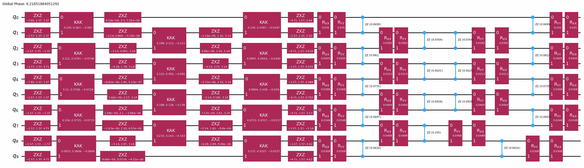
เมื่อได้พารามิเตอร์ที่ปรับแต่งแล้ว เราผูกพารามิเตอร์เหล่านั้นกับ ansatz และต่อท้ายด้วย subsequent (ไม่บีบอัด) Trotter step วงจรที่ได้มีความลึกเท่ากับ Trotter step เดียวที่บีบอัดแล้วบวก step ที่ไม่บีบอัด แต่ส่วนที่บีบอัดประมาณความแม่นยำของ Trotter step 32 step

aqc_final_circuit = aqc_ansatz.assign_parameters(aqc_final_parameters)
aqc_final_circuit.compose(subsequent_circuit, inplace=True)
aqc_final_circuit.draw("mpl", fold=-1)

Output of the previous code cell

ขั้นตอนที่ 2: ปรับแต่งปัญหาสำหรับการรันบน quantum hardware

สำหรับตัวอย่างขนาดเล็กนี้ เราใช้ fake backend (FakeKyiv) เพื่อจำลองการรันบนฮาร์ดแวร์แบบ local เรา transpile ทั้ง AQC-optimized circuit (aqc_final_circuit) และ baseline Trotter circuit (baseline_circuit ที่มี Trotter step สี่ step ตลอดเวลาวิวัฒนาการทั้งหมด ไม่มี AQC) ไปยัง instruction set architecture (ISA) ของ backend ด้วย optimization_level=3 เพื่อลด circuit depth ต่อไป

backend = FakeKyiv()

pass_manager = generate_preset_pass_manager(
    backend=backend, optimization_level=3
)

# Transpile the AQC-optimized circuit (compressed + subsequent step)
isa_circuit = pass_manager.run(aqc_final_circuit)
isa_observable = observable.apply_layout(isa_circuit.layout)
print(
    "AQC circuit depth:",
    isa_circuit.depth(lambda x: x.operation.num_qubits == 2),
)

# Transpile the baseline Trotter circuit (no AQC optimization)
isa_baseline_circuit = pass_manager.run(baseline_circuit)
isa_baseline_observable = observable.apply_layout(isa_baseline_circuit.layout)
print(
    "Baseline Trotter circuit depth:",
    isa_baseline_circuit.depth(lambda x: x.operation.num_qubits == 2),
)

AQC circuit depth: 15
Baseline Trotter circuit depth: 27

ขั้นตอนที่ 3: รันด้วย Qiskit primitives

เราใช้ primitive EstimatorV2 กับ fake backend เพื่อรันทั้ง AQC-optimized circuit และ baseline Trotter circuit วัด ZZ observable สำหรับแต่ละ circuit

estimator = Estimator(backend)

# Run both circuits
aqc_result = estimator.run([(isa_circuit, isa_observable)]).result()
baseline_result = estimator.run(
    [(isa_baseline_circuit, isa_baseline_observable)]
).result()

ขั้นตอนที่ 4: ประมวลผลและแสดงผลลัพธ์ในรูปแบบที่ต้องการ

เราดึงค่า expectation value จากทั้งสอง run และเปรียบเทียบกับผลแม่นยำ baseline Trotter circuit แสดงสิ่งที่เราจะได้โดยไม่มี AQC ที่ความลึกของวงจรเดียวกัน ในขณะที่ AQC circuit แสดงการปรับปรุงจากการปรับแต่งด้วย tensor-network

aqc_expval = aqc_result[0].data.evs.tolist()
baseline_expval = baseline_result[0].data.evs.tolist()

print(f"Exact:              {exact_expval:.4f}")
print(
    f"Baseline Trotter:   {baseline_expval:.4f}, |\u0394| = {np.abs(exact_expval - baseline_expval):.4f}  (depth {isa_baseline_circuit.depth(lambda x: x.operation.num_qubits == 2)}, {baseline_num_trotter_steps} steps)"
)
print(
    f"AQC (3+1):          {aqc_expval:.4f}, |\u0394| = {np.abs(exact_expval - aqc_expval):.4f}  (depth {isa_circuit.depth(lambda x: x.operation.num_qubits == 2)}, compressed+subsequent)"
)

Exact:              -0.7009
Baseline Trotter:   -0.5400, |Δ| = 0.1609  (depth 27, 4 steps)
AQC (3+1):          -0.5728, |Δ| = 0.1281  (depth 15, compressed+subsequent)

plt.style.use("seaborn-v0_8")

labels = [
    f"Baseline Trotter\n({baseline_num_trotter_steps} steps, depth {isa_baseline_circuit.depth(lambda x: x.operation.num_qubits == 2)})",
    f"AQC (3+1)\n(depth {isa_circuit.depth(lambda x: x.operation.num_qubits == 2)})",
]
values = [baseline_expval, aqc_expval]
colors = ["tab:orange", "tab:blue"]

plt.figure(figsize=(8, 5))
bars = plt.bar(labels, values, color=colors, width=0.5)
plt.axhline(
    y=exact_expval,
    color="tab:green",
    linestyle="--",
    linewidth=2,
    label=f"Exact ({exact_expval:.4f})",
)
plt.ylabel("Expected Value")
plt.title(
    "AQC-Tensor (3 compressed + 1 uncompressed) vs Baseline Trotter (10-site XXZ)"
)
plt.legend()
for bar in bars:
    y_val = bar.get_height()
    plt.text(
        bar.get_x() + bar.get_width() / 2.0,
        y_val,
        f"{y_val:.4f}",
        ha="center",
        va="bottom" if y_val >= 0 else "top",
    )
plt.axhline(y=0, color="black", linewidth=0.3)
plt.tight_layout()
plt.show()

Output of the previous code cell

ตัวอย่างขนาดใหญ่บนฮาร์ดแวร์จริง

ตอนนี้เราขยายไปยังโมเดล XXZ แบบ 50 ไซต์เพื่อสาธิต AQC-Tensor บนปัญหาที่มีขนาดสมจริงกว่า workflow เหมือนกับตัวอย่างขนาดเล็ก: เราบีบอัด Trotter step สาม step ผ่าน AQC และต่อท้ายด้วยหนึ่ง step ที่ไม่บีบอัด

สำหรับระบบขนาดนี้ การ exponentiation matrix ไม่สามารถทำได้ ( $2^{50}$ มิติ) ดังนั้นเราคำนวณค่า reference expectation value โดยตรงจาก MPS ที่มีความแม่นยำสูงซึ่งวิวัฒน์ตลอดเวลาทั้งหมด

ขั้นตอนที่ 1–4 รวมกัน

# -------------------------Step 1-------------------------

# Define the 50-site spin chain
L = 50
edge_list = [(i - 1, i) for i in range(1, L)]
even_edges = edge_list[::2]
odd_edges = edge_list[1::2]
coupling_map = CouplingMap(edge_list)

# Random XXZ Hamiltonian
np.random.seed(0)
Js = np.random.rand(L - 1) + 0.5 * np.ones(L - 1)
hamiltonian = SparsePauliOp(Pauli("I" * L))
for i, edge in enumerate(even_edges + odd_edges):
    hamiltonian += SparsePauliOp.from_sparse_list(
        [
            ("XX", (edge), Js[i] / 2),
            ("YY", (edge), Js[i] / 2),
            ("ZZ", (edge), Js[i]),
        ],
        num_qubits=L,
    )

observable = SparsePauliOp.from_sparse_list(
    [("ZZ", (L // 2 - 1, L // 2), 1.0)], num_qubits=L
)

# Initial Néel state
initial_state_circuit = QuantumCircuit(L)
for i in range(L):
    if i % 2:
        initial_state_circuit.x(i)

# Time parameters
aqc_evolution_time = 0.2
subsequent_evolution_time = aqc_evolution_time / 3
total_evolution_time = aqc_evolution_time + subsequent_evolution_time

# AQC target circuit (high-accuracy, 32 Trotter steps for AQC portion)
aqc_target_num_trotter_steps = 32

aqc_target_circuit = initial_state_circuit.copy()
aqc_target_circuit.compose(
    generate_time_evolution_circuit(
        hamiltonian,
        synthesis=SuzukiTrotter(reps=aqc_target_num_trotter_steps),
        time=aqc_evolution_time,
    ),
    inplace=True,
)

# Generate ansatz from 1-step Trotter circuit
aqc_good_circuit = initial_state_circuit.copy()
aqc_good_circuit.compose(
    generate_time_evolution_circuit(
        hamiltonian,
        synthesis=SuzukiTrotter(reps=1),
        time=aqc_evolution_time,
    ),
    inplace=True,
)

aqc_ansatz, aqc_initial_parameters = generate_ansatz_from_circuit(
    aqc_good_circuit
)

# Subsequent circuit: 1 non-compressed Trotter step
subsequent_circuit = generate_time_evolution_circuit(
    hamiltonian,
    synthesis=SuzukiTrotter(reps=1),
    time=subsequent_evolution_time,
)

# Baseline Trotter circuit: 4 Trotter steps over total evolution time, no AQC
baseline_num_trotter_steps = 4
baseline_circuit = initial_state_circuit.copy()
baseline_circuit.compose(
    generate_time_evolution_circuit(
        hamiltonian,
        synthesis=SuzukiTrotter(reps=baseline_num_trotter_steps),
        time=total_evolution_time,
    ),
    inplace=True,
)
print(
    f"Target circuit:  depth {aqc_target_circuit.depth(lambda x: x.operation.num_qubits == 2)}"
)
print(
    f"Ansatz circuit:  depth {aqc_ansatz.depth(lambda x: x.operation.num_qubits == 2)}, with {len(aqc_initial_parameters)} parameters"
)
print(
    f"Subsequent circuit: depth {subsequent_circuit.depth(lambda x: x.operation.num_qubits == 2)}"
)
print(
    f"Baseline circuit:   depth {baseline_circuit.depth(lambda x: x.operation.num_qubits == 2)} ({baseline_num_trotter_steps} steps, time={total_evolution_time:.4f})"
)

# Build target MPS and compute reference expectation value
simulator_settings = QuimbSimulator(
    quimb.tensor.CircuitMPS, autodiff_backend="jax"
)
aqc_target_mps = tensornetwork_from_circuit(
    aqc_target_circuit, simulator_settings
)
print("Target MPS maximum bond dimension:", aqc_target_mps.psi.max_bond())

# For the reference expectation value, we need the full evolution (AQC + subsequent)
# Build a high-accuracy full circuit for MPS reference
full_target_circuit = initial_state_circuit.copy()
full_target_circuit.compose(
    generate_time_evolution_circuit(
        hamiltonian,
        synthesis=SuzukiTrotter(reps=aqc_target_num_trotter_steps),
        time=total_evolution_time,
    ),
    inplace=True,
)
full_target_mps = tensornetwork_from_circuit(
    full_target_circuit, simulator_settings
)
exact_expval = full_target_mps.local_expectation(
    quimb.pauli("Z") & quimb.pauli("Z"), (L // 2 - 1, L // 2)
).real.item()
print(f"Reference expectation value (from MPS): {exact_expval:.6f}")

# Optimize ansatz parameters
objective = MaximizeStateFidelity(
    aqc_target_mps, aqc_ansatz, simulator_settings
)

def callback(intermediate_result: OptimizeResult):
    fidelity = 1 - intermediate_result.fun
    print(
        f"{datetime.datetime.now()} Intermediate result: Fidelity {fidelity:.8f}"
    )

result = minimize(
    objective,
    aqc_initial_parameters,
    method="L-BFGS-B",
    jac=True,
    options={"maxiter": 500},
    callback=callback,
)
if result.status not in (0, 1, 99):
    raise RuntimeError(
        f"Optimization failed: {result.message} (status={result.status})"
    )
print(f"Done after {result.nit} iterations.")

# Assemble the final AQC circuit: optimized ansatz + subsequent Trotter step
aqc_final_circuit = aqc_ansatz.assign_parameters(result.x)
aqc_final_circuit.compose(subsequent_circuit, inplace=True)

# -------------------------Step 2-------------------------

service = QiskitRuntimeService()
backend = service.least_busy(min_num_qubits=127)
print(backend)

pass_manager = generate_preset_pass_manager(
    backend=backend, optimization_level=3
)
isa_circuit = pass_manager.run(aqc_final_circuit)
isa_observable = observable.apply_layout(isa_circuit.layout)
print(
    "AQC circuit depth:",
    isa_circuit.depth(lambda x: x.operation.num_qubits == 2),
)

# Also transpile the baseline Trotter circuit (4 Trotter steps, no AQC)
isa_baseline_circuit = pass_manager.run(baseline_circuit)
isa_baseline_observable = observable.apply_layout(isa_baseline_circuit.layout)
print(
    "Baseline Trotter circuit depth:",
    isa_baseline_circuit.depth(lambda x: x.operation.num_qubits == 2),
)

# -------------------------Step 3-------------------------

# Submit both circuits in a single job
estimator = Estimator(backend)
estimator.options.environment.job_tags = ["TUT_AQCTE"]

job = estimator.run(
    [
        (isa_circuit, isa_observable),
        (isa_baseline_circuit, isa_baseline_observable),
    ]
)
print("Job ID:", job.job_id())

Target circuit:  depth 385
Ansatz circuit:  depth 7, with 816 parameters
Subsequent circuit: depth 12
Baseline circuit:   depth 49 (4 steps, time=0.2667)
Target MPS maximum bond dimension: 5
Reference expectation value (from MPS): -0.738669
2026-05-18 13:02:11.219150 Intermediate result: Fidelity 0.99795732
2026-05-18 13:02:11.232256 Intermediate result: Fidelity 0.99822481
2026-05-18 13:02:11.245160 Intermediate result: Fidelity 0.99829520
2026-05-18 13:02:11.257765 Intermediate result: Fidelity 0.99832379
2026-05-18 13:02:11.270280 Intermediate result: Fidelity 0.99836416
2026-05-18 13:02:11.284116 Intermediate result: Fidelity 0.99840073
2026-05-18 13:02:11.296856 Intermediate result: Fidelity 0.99846863
2026-05-18 13:02:11.309602 Intermediate result: Fidelity 0.99865244
2026-05-18 13:02:11.322012 Intermediate result: Fidelity 0.99872665
2026-05-18 13:02:11.334195 Intermediate result: Fidelity 0.99892335
2026-05-18 13:02:11.346570 Intermediate result: Fidelity 0.99901045
2026-05-18 13:02:11.359202 Intermediate result: Fidelity 0.99907181
2026-05-18 13:02:11.371511 Intermediate result: Fidelity 0.99911125
2026-05-18 13:02:11.383870 Intermediate result: Fidelity 0.99918585
2026-05-18 13:02:11.396184 Intermediate result: Fidelity 0.99921504
2026-05-18 13:02:11.408543 Intermediate result: Fidelity 0.99924936
2026-05-18 13:02:11.422557 Intermediate result: Fidelity 0.99929226
2026-05-18 13:02:11.436275 Intermediate result: Fidelity 0.99933099
2026-05-18 13:02:11.449511 Intermediate result: Fidelity 0.99935792
2026-05-18 13:02:11.462093 Intermediate result: Fidelity 0.99937925
2026-05-18 13:02:11.475783 Intermediate result: Fidelity 0.99940690
2026-05-18 13:02:11.490254 Intermediate result: Fidelity 0.99944409
2026-05-18 13:02:11.503292 Intermediate result: Fidelity 0.99946840
2026-05-18 13:02:11.516064 Intermediate result: Fidelity 0.99949378
2026-05-18 13:02:11.532861 Intermediate result: Fidelity 0.99951380
2026-05-18 13:02:11.546182 Intermediate result: Fidelity 0.99955313
2026-05-18 13:02:11.559168 Intermediate result: Fidelity 0.99955707
2026-05-18 13:02:11.571753 Intermediate result: Fidelity 0.99959306
2026-05-18 13:02:11.584257 Intermediate result: Fidelity 0.99960486
2026-05-18 13:02:11.597610 Intermediate result: Fidelity 0.99961714
2026-05-18 13:02:11.610106 Intermediate result: Fidelity 0.99962953
2026-05-18 13:02:11.622515 Intermediate result: Fidelity 0.99963525
2026-05-18 13:02:11.635543 Intermediate result: Fidelity 0.99964658
2026-05-18 13:02:11.649044 Intermediate result: Fidelity 0.99965027
2026-05-18 13:02:11.664148 Intermediate result: Fidelity 0.99965802
2026-05-18 13:02:11.678033 Intermediate result: Fidelity 0.99966731
2026-05-18 13:02:11.692714 Intermediate result: Fidelity 0.99967780
2026-05-18 13:02:11.706753 Intermediate result: Fidelity 0.99968567
2026-05-18 13:02:11.720780 Intermediate result: Fidelity 0.99969139
2026-05-18 13:02:11.733471 Intermediate result: Fidelity 0.99969628
2026-05-18 13:02:11.745998 Intermediate result: Fidelity 0.99970331
2026-05-18 13:02:11.758424 Intermediate result: Fidelity 0.99970796
2026-05-18 13:02:11.771986 Intermediate result: Fidelity 0.99971165
2026-05-18 13:02:11.785841 Intermediate result: Fidelity 0.99971892
2026-05-18 13:02:11.799105 Intermediate result: Fidelity 0.99972226
2026-05-18 13:02:11.811623 Intermediate result: Fidelity 0.99972441
2026-05-18 13:02:11.824114 Intermediate result: Fidelity 0.99972679
2026-05-18 13:02:11.837179 Intermediate result: Fidelity 0.99972965
2026-05-18 13:02:12.345479 Intermediate result: Fidelity 0.99972965
Done after 49 iterations.
<IBMBackend('ibm_pittsburgh')>
AQC circuit depth: 71
Baseline Trotter circuit depth: 111
Job ID: d85kc6o0bvlc73d5nhn0

# -------------------------Step 4-------------------------

hw_results = job.result()
aqc_expval = hw_results[0].data.evs.tolist()
baseline_expval = hw_results[1].data.evs.tolist()

print(f"Exact (MPS):        {exact_expval:.4f}")
print(
    f"Baseline Trotter:   {baseline_expval:.4f}, |\u0394| = {np.abs(exact_expval - baseline_expval):.4f}"
)
print(
    f"AQC (3+1):          {aqc_expval:.4f}, |\u0394| = {np.abs(exact_expval - aqc_expval):.4f}"
)

labels = [
    f"Baseline Trotter\n({baseline_num_trotter_steps} steps, depth {isa_baseline_circuit.depth(lambda x: x.operation.num_qubits == 2)})",
    f"AQC (3+1)\n(depth {isa_circuit.depth(lambda x: x.operation.num_qubits == 2)})",
]
values = [baseline_expval, aqc_expval]
colors = ["tab:orange", "tab:blue"]

plt.figure(figsize=(8, 5))
bars = plt.bar(labels, values, color=colors, width=0.5)
plt.axhline(
    y=exact_expval,
    color="tab:green",
    linestyle="--",
    linewidth=2,
    label=f"Exact ({exact_expval:.4f})",
)
plt.ylabel("Expected Value")
plt.title(
    "AQC-Tensor (3 compressed + 1 uncompressed) vs Baseline Trotter (50-site XXZ)"
)
plt.legend()
for bar in bars:
    y_val = bar.get_height()
    plt.text(
        bar.get_x() + bar.get_width() / 2.0,
        y_val,
        f"{y_val:.4f}",
        ha="center",
        va="bottom" if y_val >= 0 else "top",
    )
plt.axhline(y=0, color="black", linewidth=0.3)
plt.tight_layout()
plt.show()

Exact (MPS):        -0.7387
Baseline Trotter:   -0.5955, |Δ| = 0.1432
AQC (3+1):          -0.6734, |Δ| = 0.0653

Output of the previous code cell

ขั้นตอนถัดไป

คำแนะนำ

ถ้าคุณสนใจในงานนี้ อาจสนใจเนื้อหาต่อไปนี้ด้วย:

AQC-Tensor addon documentation — รวมเทคนิค unitary AQC ที่เกี่ยวข้อง ซึ่งปรับแต่ง parametrized circuit เพื่อประมาณ target unitary operator แทนที่จะเป็น prepared state
เทคนิคการลดและกำจัด error
รวมเทคนิคการลด error

แหล่งที่มา: IBM Quantum docs — อัปเดตเมื่อ 10 มิ.ย. 2569

เวอร์ชันภาษาอังกฤษ บน doQumentation — อัปเดตเมื่อ 10 มิ.ย. 2569

การแปลนี้อิงตามเวอร์ชันภาษาอังกฤษวันที่ 9 เม.ย. 2569

ผลการเรียนรู้​

สิ่งที่ควรรู้ก่อน​

ภูมิหลัง​

AQC-Tensor ทำงานอย่างไร​

เมื่อไหรที่ควรใช้ AQC-Tensor​

ข้อกำหนดเบื้องต้น​

การตั้งค่า​

ตัวอย่างขนาดเล็กด้วย simulator​

ขั้นตอนที่ 1: แมป input แบบคลาสสิกไปยังปัญหาควอนตัม​

ตั้งค่า Hamiltonian, observable และสถานะเริ่มต้น​

คำนวณค่า expectation value ที่แม่นยำ​

สร้าง AQC target circuit​

สร้าง ansatz, พารามิเตอร์เริ่มต้น, subsequent circuit และ baseline circuit​

ตั้งค่าการจำลอง tensor network และสร้าง target MPS​

ปรับแต่งพารามิเตอร์ ansatz​

ประกอบ AQC circuit สุดท้าย​

ขั้นตอนที่ 2: ปรับแต่งปัญหาสำหรับการรันบน quantum hardware​

ขั้นตอนที่ 3: รันด้วย Qiskit primitives​

ขั้นตอนที่ 4: ประมวลผลและแสดงผลลัพธ์ในรูปแบบที่ต้องการ​

ตัวอย่างขนาดใหญ่บนฮาร์ดแวร์จริง​

ขั้นตอนที่ 1–4 รวมกัน​

ขั้นตอนถัดไป​

ผลการเรียนรู้

สิ่งที่ควรรู้ก่อน

ภูมิหลัง

AQC-Tensor ทำงานอย่างไร

เมื่อไหรที่ควรใช้ AQC-Tensor

ข้อกำหนดเบื้องต้น

การตั้งค่า

ตัวอย่างขนาดเล็กด้วย simulator

ขั้นตอนที่ 1: แมป input แบบคลาสสิกไปยังปัญหาควอนตัม

ตั้งค่า Hamiltonian, observable และสถานะเริ่มต้น

คำนวณค่า expectation value ที่แม่นยำ

สร้าง AQC target circuit

สร้าง ansatz, พารามิเตอร์เริ่มต้น, subsequent circuit และ baseline circuit

ตั้งค่าการจำลอง tensor network และสร้าง target MPS

ปรับแต่งพารามิเตอร์ ansatz

ประกอบ AQC circuit สุดท้าย

ขั้นตอนที่ 2: ปรับแต่งปัญหาสำหรับการรันบน quantum hardware

ขั้นตอนที่ 3: รันด้วย Qiskit primitives

ขั้นตอนที่ 4: ประมวลผลและแสดงผลลัพธ์ในรูปแบบที่ต้องการ

ตัวอย่างขนาดใหญ่บนฮาร์ดแวร์จริง

ขั้นตอนที่ 1–4 รวมกัน

ขั้นตอนถัดไป