การ Benchmark แบบ Real-time เพื่อเลือก Qubit

ประมาณการใช้งาน: 4 นาทีบน Eagle r2 processor (หมายเหตุ: นี่เป็นเพียงการประมาณเท่านั้น เวลาจริงอาจแตกต่างกัน)

# Added by doQumentation — required packages for this notebook
!pip install -q matplotlib numpy qiskit qiskit-experiments qiskit-ibm-runtime rustworkx

# This cell is hidden from users – it disables some lint rules
# ruff: noqa: E722

พื้นหลัง

บทแนะนำนี้แสดงวิธีรันการทดลอง characterization แบบ real-time และอัปเดต backend properties เพื่อปรับปรุงการเลือก Qubit เมื่อแมป Circuit ไปยัง physical qubit บน QPU คุณจะได้เรียนรู้การทดลอง characterization พื้นฐานที่ใช้กำหนด properties ของ QPU วิธีทำสิ่งเหล่านี้ใน Qiskit และวิธีอัปเดต properties ที่บันทึกไว้ใน backend object ที่แทน QPU ตามผลการทดลอง

QPU-reported properties จะอัปเดตวันละครั้ง แต่ระบบอาจเปลี่ยนแปลงเร็วกว่าช่วงเวลาระหว่างการอัปเดต สิ่งนี้อาจส่งผลต่อความน่าเชื่อถือของ qubit selection routines ในขั้นตอน Layout ของ pass manager เนื่องจากใช้ reported properties ที่ไม่สะท้อนสถานะปัจจุบันของ QPU ด้วยเหตุนี้ อาจคุ้มค่าที่จะใช้เวลา QPU บางส่วนไปกับการทดลอง characterization ซึ่งสามารถนำมาใช้อัปเดต QPU properties ที่ใช้โดย Layout routine ได้

สิ่งที่ต้องมี

ก่อนเริ่มบทแนะนำนี้ ตรวจสอบให้แน่ใจว่าติดตั้งสิ่งต่อไปนี้แล้ว:

• Qiskit SDK v2.0 หรือใหม่กว่า พร้อมรองรับ visualization
• Qiskit Runtime v0.40 หรือใหม่กว่า ( pip install qiskit-ibm-runtime )
• Qiskit Experiments v0.12 หรือใหม่กว่า ( pip install qiskit-experiments )
• Rustworkx graph library (pip install rustworkx)

ตั้งค่า

from qiskit_ibm_runtime import SamplerV2
from qiskit.transpiler import generate_preset_pass_manager
from qiskit.quantum_info import hellinger_fidelity
from qiskit.transpiler import InstructionProperties

from qiskit_experiments.library import (
    T1,
    T2Hahn,
    LocalReadoutError,
    StandardRB,
)
from qiskit_experiments.framework import BatchExperiment, ParallelExperiment

from qiskit_ibm_runtime import QiskitRuntimeService
from qiskit_ibm_runtime import Session

from datetime import datetime
from collections import defaultdict
import numpy as np
import rustworkx
import matplotlib.pyplot as plt
import copy

ขั้นตอนที่ 1: แมป input แบบ classical ไปยังปัญหา quantum

เพื่อ benchmark ความแตกต่างด้านประสิทธิภาพ เราพิจารณา Circuit ที่เตรียม Bell state ข้าม linear chain ที่มีความยาวต่างกัน โดยวัด fidelity ของ Bell state ที่ปลายทั้งสองของ chain

from qiskit import QuantumCircuit

ideal_dist = {"00": 0.5, "11": 0.5}

num_qubits_list = [10, 20, 30, 40, 50, 60, 70, 80, 90, 100, 110, 120, 127]
circuits = []
for num_qubits in num_qubits_list:
    circuit = QuantumCircuit(num_qubits, 2)
    circuit.h(0)
    for i in range(num_qubits - 1):
        circuit.cx(i, i + 1)
    circuit.barrier()
    circuit.measure(0, 0)
    circuit.measure(num_qubits - 1, 1)
    circuits.append(circuit)

circuits[-1].draw(output="mpl", style="clifford", fold=-1)

ตั้งค่า Backend และ coupling map

ก่อนอื่น เลือก Backend

# To run on hardware, select the backend with the fewest number of jobs in the queue
service = QiskitRuntimeService()
backend = service.least_busy(
    operational=True, simulator=False, min_num_qubits=127
)

qubits = list(range(backend.num_qubits))

จากนั้นดึง coupling map ของมัน

coupling_graph = backend.coupling_map.graph.to_undirected(multigraph=False)

# Get unidirectional coupling map
one_dir_coupling_map = coupling_graph.edge_list()

เพื่อ benchmark two-qubit Gate ให้ได้มากที่สุดพร้อมกัน เราแยก coupling map ออกเป็น layered_coupling_map object นี้ประกอบด้วยรายการของ layer โดยแต่ละ layer คือรายการ edge ที่สามารถรัน two-qubit Gate พร้อมกันได้ วิธีนี้เรียกอีกอย่างว่า edge coloring ของ coupling map

# Get layered coupling map
edge_coloring = rustworkx.graph_bipartite_edge_color(coupling_graph)
layered_coupling_map = defaultdict(list)
for edge_idx, color in edge_coloring.items():
    layered_coupling_map[color].append(
        coupling_graph.get_edge_endpoints_by_index(edge_idx)
    )
layered_coupling_map = [
    sorted(layered_coupling_map[i])
    for i in sorted(layered_coupling_map.keys())
]

การทดลอง Characterization

มีการใช้ชุดการทดลองเพื่อ characterize คุณสมบัติหลักของ Qubit ใน QPU ซึ่งได้แก่ $T_1$, $T_2$, readout error และ single-qubit กับ two-qubit gate error เราจะสรุปสั้น ๆ ว่าคุณสมบัติเหล่านี้คืออะไร และอ้างอิงการทดลองใน package qiskit-experiments ที่ใช้ characterize สิ่งเหล่านี้

T1

$T_1$ คือเวลาลักษณะที่ใช้สำหรับ Qubit ที่ถูกกระตุ้นให้ตกกลับสู่ ground state เนื่องจากกระบวนการ decoherence แบบ amplitude-damping ใน การทดลอง $T_1$ เราวัด Qubit ที่ถูกกระตุ้นหลังจากหน่วงเวลา ยิ่งหน่วงเวลานานขึ้น Qubit ก็ยิ่งมีโอกาสตกลงสู่ ground state มากขึ้น เป้าหมายของการทดลองคือ characterize อัตราการ decay ของ Qubit ไปยัง ground state

T2

$T_2$ แสดงถึงช่วงเวลาที่ Bloch vector projection ของ Qubit เดี่ยวบนระนาบ XY ลดลงเหลือประมาณ 37% ($\frac{1}{e}$) ของ amplitude เริ่มต้น เนื่องจากกระบวนการ decoherence แบบ dephasing ใน การทดลอง $T_2$ Hahn Echo เราสามารถประมาณอัตราการ decay นี้ได้

การ characterize ความผิดพลาด State preparation and measurement (SPAM)

ใน การทดลอง characterize ความผิดพลาด SPAM Qubit จะถูกเตรียมในสถานะหนึ่ง ($\vert 0 \rangle$ หรือ $\vert 1 \rangle$) และวัด ความน่าจะเป็นของการวัดสถานะที่ต่างจากสถานะที่เตรียมไว้จะให้ความน่าจะเป็นของความผิดพลาด

Randomized benchmarking สำหรับ single-qubit และ two-qubit

Randomized benchmarking (RB) เป็น protocol ยอดนิยมสำหรับ characterize อัตราความผิดพลาดของ quantum processor การทดลอง RB ประกอบด้วยการสร้าง random Clifford Circuit บน Qubit ที่กำหนด โดย unitary ที่ Circuit คำนวณได้คือ identity หลังจากรัน Circuit นับจำนวน shot ที่เกิดความผิดพลาด (นั่นคือ output ที่แตกต่างจาก ground state) และจากข้อมูลนี้สามารถอนุมานประมาณการความผิดพลาดสำหรับอุปกรณ์ quantum ได้โดยการคำนวณ Error Per Clifford

# Create T1 experiments on all qubit in parallel
t1_exp = ParallelExperiment(
    [
        T1(
            physical_qubits=[qubit],
            delays=[1e-6, 20e-6, 40e-6, 80e-6, 200e-6, 400e-6],
        )
        for qubit in qubits
    ],
    backend,
    analysis=None,
)

# Create T2-Hahn experiments on all qubit in parallel
t2_exp = ParallelExperiment(
    [
        T2Hahn(
            physical_qubits=[qubit],
            delays=[1e-6, 20e-6, 40e-6, 80e-6, 200e-6, 400e-6],
        )
        for qubit in qubits
    ],
    backend,
    analysis=None,
)

# Create readout experiments on all qubit in parallel
readout_exp = LocalReadoutError(qubits)

# Create single-qubit RB experiments on all qubit in parallel
singleq_rb_exp = ParallelExperiment(
    [
        StandardRB(
            physical_qubits=[qubit], lengths=[10, 100, 500], num_samples=10
        )
        for qubit in qubits
    ],
    backend,
    analysis=None,
)

# Create two-qubit RB experiments on the three layers of disjoint edges of the heavy-hex
twoq_rb_exp_batched = BatchExperiment(
    [
        ParallelExperiment(
            [
                StandardRB(
                    physical_qubits=pair,
                    lengths=[10, 50, 100],
                    num_samples=10,
                )
                for pair in layer
            ],
            backend,
            analysis=None,
        )
        for layer in layered_coupling_map
    ],
    backend,
    flatten_results=True,
    analysis=None,
)

QPU properties ตามช่วงเวลา

เมื่อดู reported QPU properties ตามช่วงเวลา (เราจะพิจารณาช่วงหนึ่งสัปดาห์ด้านล่าง) จะเห็นว่าสิ่งเหล่านี้สามารถผันผวนได้ในระดับวันเดียว ความผันผวนเล็กน้อยอาจเกิดขึ้นได้แม้ภายในวันเดียวกัน ในสถานการณ์นี้ reported properties (อัปเดตวันละครั้ง) จะไม่สะท้อนสถานะปัจจุบันของ QPU ได้อย่างแม่นยำ ยิ่งกว่านั้น หาก job ถูก transpile ในเครื่อง (โดยใช้ reported properties ปัจจุบัน) แล้ว submit แต่รันในภายหลัง (ไม่ว่าจะเป็นนาทีหรือวัน) ก็อาจเสี่ยงที่จะใช้ properties ที่ล้าสมัยในการเลือก Qubit ระหว่างขั้นตอน transpilation สิ่งนี้แสดงให้เห็นถึงความสำคัญของการมีข้อมูลที่อัปเดตเกี่ยวกับ QPU ณ เวลาที่รัน ก่อนอื่น มาดึง properties ในช่วงเวลาหนึ่งกัน

instruction_2q_name = "cz"  # set the name of the default 2q of the device
errors_list = []
for day_idx in range(10, 17):
    calibrations_time = datetime(
        year=2025, month=8, day=day_idx, hour=0, minute=0, second=0
    )
    targer_hist = backend.target_history(datetime=calibrations_time)

    t1_dict, t2_dict = {}, {}
    for qubit in range(targer_hist.num_qubits):
        t1_dict[qubit] = targer_hist.qubit_properties[qubit].t1
        t2_dict[qubit] = targer_hist.qubit_properties[qubit].t2

    errors_dict = {
        "1q": targer_hist["sx"],
        "2q": targer_hist[f"{instruction_2q_name}"],
        "spam": targer_hist["measure"],
        "t1": t1_dict,
        "t2": t2_dict,
    }

    errors_list.append(errors_dict)

จากนั้น มา plot ค่าต่าง ๆ กัน

fig, axs = plt.subplots(5, 1, figsize=(10, 20), sharex=False)

# Plot for T1 values
for qubit in range(targer_hist.num_qubits):
    t1s = []
    for errors_dict in errors_list:
        t1_dict = errors_dict["t1"]
        try:
            t1s.append(t1_dict[qubit] / 1e-6)
        except:
            print(f"missing t1 data for qubit {qubit}")

    axs[0].plot(t1s)

axs[0].set_title("T1")
axs[0].set_ylabel(r"Time ($\mu s$)")
axs[0].set_xlabel("Days")

# Plot for T2 values
for qubit in range(targer_hist.num_qubits):
    t2s = []
    for errors_dict in errors_list:
        t2_dict = errors_dict["t2"]
        try:
            t2s.append(t2_dict[qubit] / 1e-6)
        except:
            print(f"missing t2 data for qubit {qubit}")

    axs[1].plot(t2s)

axs[1].set_title("T2")
axs[1].set_ylabel(r"Time ($\mu s$)")
axs[1].set_xlabel("Days")

# Plot SPAM values
for qubit in range(targer_hist.num_qubits):
    spams = []
    for errors_dict in errors_list:
        spam_dict = errors_dict["spam"]
        spams.append(spam_dict[tuple([qubit])].error)

    axs[2].plot(spams)

axs[2].set_title("SPAM Errors")
axs[2].set_ylabel("Error Rate")
axs[2].set_xlabel("Days")

# Plot 1Q Gate Errors
for qubit in range(targer_hist.num_qubits):
    oneq_gates = []
    for errors_dict in errors_list:
        oneq_gate_dict = errors_dict["1q"]
        oneq_gates.append(oneq_gate_dict[tuple([qubit])].error)

    axs[3].plot(oneq_gates)

axs[3].set_title("1Q Gate Errors")
axs[3].set_ylabel("Error Rate")
axs[3].set_xlabel("Days")

# Plot 2Q Gate Errors
for pair in one_dir_coupling_map:
    twoq_gates = []
    for errors_dict in errors_list:
        twoq_gate_dict = errors_dict["2q"]
        twoq_gates.append(twoq_gate_dict[pair].error)

    axs[4].plot(twoq_gates)

axs[4].set_title("2Q Gate Errors")
axs[4].set_ylabel("Error Rate")
axs[4].set_xlabel("Days")

plt.subplots_adjust(hspace=0.5)
plt.show()

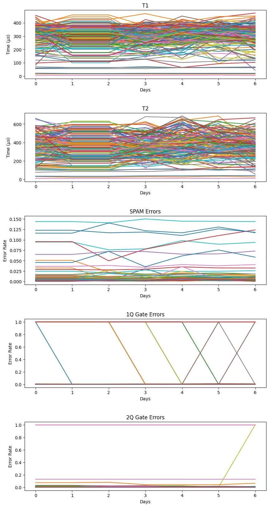
จะเห็นได้ว่าในช่วงหลายวัน คุณสมบัติบางอย่างของ Qubit อาจเปลี่ยนแปลงได้อย่างมีนัยสำคัญ สิ่งนี้แสดงให้เห็นถึงความสำคัญของการมีข้อมูลที่สดใหม่เกี่ยวกับสถานะ QPU เพื่อให้สามารถเลือก Qubit ที่ทำงานได้ดีที่สุดสำหรับการทดลอง

Step 2: ปรับปัญหาให้เหมาะสมสำหรับการรันบนฮาร์ดแวร์ควอนตัม

ในบทเรียนนี้ไม่มีการปรับแต่ง Circuit หรือ Operator ใดๆ

Step 3: รันโดยใช้ Qiskit primitives

รัน Circuit ควอนตัมด้วยการเลือก Qubit แบบค่าเริ่มต้น

เพื่อใช้เป็นผลอ้างอิงด้านประสิทธิภาพ เราจะรัน Circuit ควอนตัมบน QPU โดยใช้ Qubit แบบค่าเริ่มต้น ซึ่งเป็น Qubit ที่ถูกเลือกตามคุณสมบัติของ Backend ที่ร้องขอ เราจะใช้ optimization_level = 3 ซึ่งเป็นการตั้งค่าที่รวมการปรับแต่งการ Transpile ขั้นสูงที่สุด และใช้คุณสมบัติเป้าหมาย (เช่น ค่าความผิดพลาดของการดำเนินการ) เพื่อเลือก Qubit ที่มีประสิทธิภาพดีที่สุดสำหรับการรัน

pm = generate_preset_pass_manager(target=backend.target, optimization_level=3)
isa_circuits = pm.run(circuits)
initial_qubits = [
    [
        idx
        for idx, qb in circuit.layout.initial_layout.get_physical_bits().items()
        if qb._register.name != "ancilla"
    ]
    for circuit in isa_circuits
]

รัน Circuit ควอนตัมด้วยการเลือก Qubit แบบเรียลไทม์

ในส่วนนี้ เราจะศึกษาความสำคัญของการมีข้อมูลที่อัปเดตเกี่ยวกับคุณสมบัติของ Qubit บน QPU เพื่อให้ได้ผลลัพธ์ที่ดีที่สุด ขั้นแรก เราจะทำการทดลองลักษณะเฉพาะของ QPU อย่างครบถ้วน ($T_1$, $T_2$, SPAM, single-qubit RB และ two-qubit RB) เพื่อนำมาอัปเดตคุณสมบัติของ Backend ซึ่งช่วยให้ pass manager สามารถเลือก Qubit สำหรับการรันโดยอิงจากข้อมูลล่าสุดเกี่ยวกับ QPU และอาจช่วยเพิ่มประสิทธิภาพการรัน ขั้นที่สอง เราจะรัน Circuit Bell pair และเปรียบเทียบ fidelity ที่ได้จากการเลือก Qubit ด้วยคุณสมบัติ QPU ที่อัปเดตแล้ว กับ fidelity ที่ได้ก่อนหน้าเมื่อใช้คุณสมบัติที่รายงานตามค่าเริ่มต้นในการเลือก Qubit

ข้อควรระวัง

โปรดทราบว่าการทดลองลักษณะเฉพาะบางอย่างอาจล้มเหลวเมื่อกระบวนการ fitting ไม่สามารถ fit curve กับข้อมูลที่วัดได้ หากเห็น warning จากการทดลองเหล่านี้ ให้ตรวจสอบว่าการลักษณะเฉพาะใดล้มเหลวบน Qubit ใด และลองปรับพารามิเตอร์ของการทดลอง (เช่น เวลาสำหรับ $T_1$, $T_2$ หรือจำนวนความยาวของการทดลอง RB)

# Prepare characterization experiments
batches = [t1_exp, t2_exp, readout_exp, singleq_rb_exp, twoq_rb_exp_batched]
batches_exp = BatchExperiment(batches, backend)  # , analysis=None)
run_options = {"shots": 1e3, "dynamic": False}

with Session(backend=backend) as session:
    sampler = SamplerV2(mode=session)

    # Run characterization experiments
    batches_exp_data = batches_exp.run(
        sampler=sampler, **run_options
    ).block_for_results()

    EPG_sx_result_list = batches_exp_data.analysis_results("EPG_sx")
    EPG_sx_result_q_indices = [
        result.device_components.index for result in EPG_sx_result_list
    ]
    EPG_x_result_list = batches_exp_data.analysis_results("EPG_x")
    EPG_x_result_q_indices = [
        result.device_components.index for result in EPG_x_result_list
    ]
    T1_result_list = batches_exp_data.analysis_results("T1")
    T1_result_q_indices = [
        result.device_components.index for result in T1_result_list
    ]

    T2_result_list = batches_exp_data.analysis_results("T2")
    T2_result_q_indices = [
        result.device_components.index for result in T2_result_list
    ]

    Readout_result_list = batches_exp_data.analysis_results(
        "Local Readout Mitigator"
    )

    EPG_2q_result_list = batches_exp_data.analysis_results(
        f"EPG_{instruction_2q_name}"
    )

    # Update target properties
    target = copy.deepcopy(backend.target)
    for i in range(target.num_qubits - 1):
        qarg = (i,)

        if qarg in EPG_sx_result_q_indices:
            target.update_instruction_properties(
                instruction="sx",
                qargs=qarg,
                properties=InstructionProperties(
                    error=EPG_sx_result_list[i].value.nominal_value
                ),
            )
        if qarg in EPG_x_result_q_indices:
            target.update_instruction_properties(
                instruction="x",
                qargs=qarg,
                properties=InstructionProperties(
                    error=EPG_x_result_list[i].value.nominal_value
                ),
            )

        err_mat = Readout_result_list.value.assignment_matrix(i)
        readout_assignment_error = (
            err_mat[0, 1] + err_mat[1, 0]
        ) / 2  # average readout error
        target.update_instruction_properties(
            instruction="measure",
            qargs=qarg,
            properties=InstructionProperties(error=readout_assignment_error),
        )

        if qarg in T1_result_q_indices:
            target.qubit_properties[i].t1 = T1_result_list[
                i
            ].value.nominal_value
        if qarg in T2_result_q_indices:
            target.qubit_properties[i].t2 = T2_result_list[
                i
            ].value.nominal_value

    for pair_idx, pair in enumerate(one_dir_coupling_map):
        qarg = tuple(pair)
        try:
            target.update_instruction_properties(
                instruction=instruction_2q_name,
                qargs=qarg,
                properties=InstructionProperties(
                    error=EPG_2q_result_list[pair_idx].value.nominal_value
                ),
            )
        except:
            target.update_instruction_properties(
                instruction=instruction_2q_name,
                qargs=qarg[::-1],
                properties=InstructionProperties(
                    error=EPG_2q_result_list[pair_idx].value.nominal_value
                ),
            )

    # transpile circuits to updated target
    pm = generate_preset_pass_manager(target=target, optimization_level=3)
    isa_circuit_updated = pm.run(circuits)
    updated_qubits = [
        [
            idx
            for idx, qb in circuit.layout.initial_layout.get_physical_bits().items()
            if qb._register.name != "ancilla"
        ]
        for circuit in isa_circuit_updated
    ]

    n_trials = 3  # run multiple trials to see variations

    # interleave circuits
    interleaved_circuits = []
    for original_circuit, updated_circuit in zip(
        isa_circuits, isa_circuit_updated
    ):
        interleaved_circuits.append(original_circuit)
        interleaved_circuits.append(updated_circuit)

    # Run circuits
    # Set simple error suppression/mitigation options
    sampler.options.dynamical_decoupling.enable = True
    sampler.options.dynamical_decoupling.sequence_type = "XY4"

    job_interleaved = sampler.run(interleaved_circuits * n_trials)

Step 4: ประมวลผลและส่งคืนผลลัพธ์ในรูปแบบ classical ที่ต้องการ

สุดท้าย มาเปรียบเทียบ fidelity ของ Bell state ที่ได้จากการตั้งค่าสองแบบที่แตกต่างกัน:

• original คือใช้ Qubit แบบค่าเริ่มต้นที่ Transpiler เลือกตามคุณสมบัติที่รายงานของ Backend
• updated คือใช้ Qubit ที่เลือกตามคุณสมบัติที่อัปเดตของ Backend หลังจากที่การทดลองลักษณะเฉพาะรันเสร็จแล้ว

results = job_interleaved.result()
all_fidelity_list, all_fidelity_updated_list = [], []
for exp_idx in range(n_trials):
    fidelity_list, fidelity_updated_list = [], []

    for idx, num_qubits in enumerate(num_qubits_list):
        pub_result_original = results[
            2 * exp_idx * len(num_qubits_list) + 2 * idx
        ]
        pub_result_updated = results[
            2 * exp_idx * len(num_qubits_list) + 2 * idx + 1
        ]

        fid = hellinger_fidelity(
            ideal_dist, pub_result_original.data.c.get_counts()
        )
        fidelity_list.append(fid)

        fid_up = hellinger_fidelity(
            ideal_dist, pub_result_updated.data.c.get_counts()
        )
        fidelity_updated_list.append(fid_up)
    all_fidelity_list.append(fidelity_list)
    all_fidelity_updated_list.append(fidelity_updated_list)

plt.figure(figsize=(8, 6))
plt.errorbar(
    num_qubits_list,
    np.mean(all_fidelity_list, axis=0),
    yerr=np.std(all_fidelity_list, axis=0),
    fmt="o-.",
    label="original",
    color="b",
)
# plt.plot(num_qubits_list, fidelity_list, '-.')
plt.errorbar(
    num_qubits_list,
    np.mean(all_fidelity_updated_list, axis=0),
    yerr=np.std(all_fidelity_updated_list, axis=0),
    fmt="o-.",
    label="updated",
    color="r",
)
# plt.plot(num_qubits_list, fidelity_updated_list, '-.')
plt.xlabel("Chain length")
plt.xticks(num_qubits_list)
plt.ylabel("Fidelity")
plt.title("Bell pair fidelity at the edge of N-qubits chain")
plt.legend()
plt.grid(
    alpha=0.2,
    linestyle="-.",
)
plt.show()

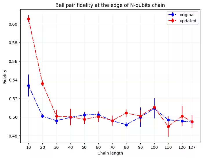
ไม่ใช่ทุกครั้งที่การรันจะแสดงให้เห็นถึงการปรับปรุงประสิทธิภาพจากการลักษณะเฉพาะแบบเรียลไทม์ และเมื่อความยาวของ chain เพิ่มขึ้น ทำให้มีอิสระในการเลือก Qubit ทางกายภาพน้อยลง ความสำคัญของข้อมูลอุปกรณ์ที่อัปเดตก็จะลดลงด้วย อย่างไรก็ตาม เป็นแนวปฏิบัติที่ดีในการเก็บข้อมูลล่าสุดเกี่ยวกับคุณสมบัติของอุปกรณ์เพื่อทำความเข้าใจประสิทธิภาพของมัน บางครั้ง two-level systems ชั่วคราวอาจส่งผลต่อประสิทธิภาพของ Qubit บางตัว ข้อมูลเรียลไทม์สามารถแจ้งให้เราทราบเมื่อเหตุการณ์ดังกล่าวเกิดขึ้น และช่วยให้เราหลีกเลี่ยงความล้มเหลวในการทดลองในกรณีเช่นนั้น

ลองทำดู

ลองนำวิธีการนี้ไปใช้กับการรันของคุณและดูว่าได้ประโยชน์มากแค่ไหน! คุณยังสามารถลองดูว่าได้รับการปรับปรุงมากแค่ไหนจาก Backend ที่แตกต่างกัน

แบบสำรวจบทเรียน

Link to survey

Note: This survey is provided by IBM Quantum and relates to the original English content. To give feedback on doQumentation's website, translations, or code execution, please open a GitHub issue.

กรุณาทำแบบสำรวจสั้นๆ นี้เพื่อให้ feedback เกี่ยวกับบทเรียนนี้ ข้อมูลเชิงลึกของคุณจะช่วยให้เราพัฒนาเนื้อหาและประสบการณ์การใช้งานได้ดียิ่งขึ้น