ปรับปรุงค่าคาดหวังด้วย propagated noise absorption (PNA)
ประมาณการใช้งาน: 10 นาทีบนโปรเซสเซอร์ Heron (หมายเหตุ: นี่เป็นเพียงการประมาณการเท่านั้น เวลาใช้งานจริงของคุณอาจแตกต่างออกไป)
ผลลัพธ์การเรียนรู้
-
propagated noise absorption (PNA) คืออะไร และมันลด noise ของ two-qubit gate ได้อย่างไรโดยการดูดซับ inverse noise channel ที่เรียนรู้มาเข้าไปใน observable ที่วัดได้
-
วิธีใช้
samplomaticเพื่อ box และใส่คำอธิบายประกอบให้กับ circuit layer สำหรับการ twirling, การเปลี่ยน basis และการฉีด noise -
วิธีเรียนรู้ layer noise ด้วย
[NoiseLearnerV3](/guides/directed-execution-model#noiselearnerv3) และแพร่กระจายเข้าไปใน observable ที่ลด noise ด้วยqiskit-addon-pna -
วิธีสุ่มตัวอย่าง randomized circuit ด้วยคลาส
QuantumProgramและExecutorในqiskit-ibm-runtimeและการรวม PNA เข้ากับ TREX และ post-selection
ข้อกำหนดเบื้องต้น
-
ขั้นตอนการทำงานของ Qiskit patterns
-
การใช้ primitive Estimator เพื่อคำนวณค่าคาดหวังของ observable
-
เทคนิคการลดข้อผิดพลาด เช่น Pauli twirling และ TREX ซึ่งครอบคลุมใน รวมตัวเลือกการลดข้อผิดพลาดกับ primitive Estimator
ความเป็นมา
ใน tutorial นี้ เราจะสาธิตวิธีใช้เครื่องมือลดข้อผิดพลาดขั้นสูงใน Qiskit เพื่อปรับปรุงการประมาณค่าคาดหวังในการทดลองควอนตัมที่มี noise
propagated noise absorption (PNA) คืออะไร?
Propagated noise absorption เป็นเทคนิคสำหรับลดข้อผิดพลาดของ gate โดยการแพร่กระจาย observable ผ่าน inverse noise channel ที่ส่งผลต่อ two-qubit gate ซึ่งส่งผลให้ได้ observable ที่ลด noise
เราสามารถใช้ quantum error mitigation เพื่อดึงค่าคาดหวังที่มีประโยชน์จาก quantum hardware ที่มี noise โดยไม่ต้องอาศัย full fault tolerance PNA มุ่งเน้นเฉพาะการดูดซับผลกระทบของ noise เข้าไปใน observable เอง แทนที่จะแก้ไขการดำเนินการของ circuit
gate ที่มี noise แต่ละตัวใน quantum circuit สามารถจำลองเป็น gate อุดมคติตามด้วย noise channel PNA เรียนรู้หรือระบุลักษณะของ noise channel เหล่านี้และกำหนด inverse ของมัน แทนที่จะแทรกการดำเนินการ inverse เข้าไปในการรันบนฮาร์ดแวร์ (ซึ่งโดยทั่วไปแล้วเป็นไปไม่ได้) PNA จะแพร่กระจาย inverse noise channel ไปข้างหน้าผ่าน circuit และนำไปใช้กับ observable กระบวนการนี้จะแปลง observable ให้เป็นตัวดำเนินการใหม่ ซึ่งการวัด บน circuit ที่มี noise จะให้ค่าคาดหวังเดียวกับการวัด บน circuit อุดมคติที่ไม่มี noise
สามารถสรุปได้ดังนี้:
- จำลอง gate ที่มี noise แต่ละตัว เป็นการดำเนินการอุดมคติตามด้วย noise channel
- เรียนรู้หรือประมาณ แต่ละตัวโดยใช้เครื่องมือระบุลักษณะ noise
- กำหนดและแพร่กระจาย inverse noise map ไปข้างหน้าผ่าน circuit โดยใช้เทคนิค Pauli transfer
- ดูดซับ inverse เหล่านี้เข้าไปใน observable ซึ่งส่งผลให้ได้ตัวดำเนินการที่ลด noise แล้ว
เมื่อ noise ถูกอธิบายเป็น Pauli channel (หรือโดยทั่วไปคือ sparse Pauli-Lindblad channel) การแพร่กระจายนี้สามารถทำได้อย่างมีประสิทธิภาพโดยใช้ Pauli propagation Pauli propagation เป็นกรอบการทำงานสำหรับประมาณว่า inverse noise channel เปลี่ยนแปลงอย่างไรเมื่อผ่าน layer ของการดำเนินการแบบ Clifford และ non-Clifford ในขณะที่ควบคุมความซับซ้อนในการคำนวณ
โดยการเปลี่ยนการลดข้อผิดพลาดไปไว้ที่ observable PNA หลีกเลี่ยง sampling overhead ขนาดใหญ่ที่จะเกิดขึ้นจากการแทรกการดำเนินการแก้ไขทางกายภาพเข้าไปใน circuit แทนที่จะเป็นเช่นนั้น circuit ที่มี noise ดั้งเดิมจะถูกรัน ในขณะที่ observable ถูกแปลงเป็นตัวดำเนินการใหม่ ซึ่งค่าคาดหวังของมันจะหักล้างผลกระทบของ noise
ขั้นตอนการทำงานของ PNA
กระบวนการนี้สามารถเข้าใจได้ผ่านขั้นตอนเชิงแนวคิดต่อไปนี้ แผนภาพแรกแสดงการทดลองที่มี noise แบบมาตรฐาน

หากเราเรียนรู้ noise model เราสามารถใช้ inverse ของมันและหักล้าง noise ได้

แทนที่จะดำเนินการ inverse noise channel โดยการสุ่มตัวอย่างบน QPU เหมือนใน probabilistic error cancellation (PEC) เรานำไปใช้แบบคลาสสิกกับ observable ที่วัดได้โดยใช้ Pauli propagation observable ที่ได้จะช่วยลด gate noise ที่เรียนรู้มาได้อย่างมีประสิทธิภาพเมื่อวัด

การลดข้อผิดพลาดแบบโมดูลาร์ด้วย Samplomatic และ Executor
แนวทาง PNA ต่อยอดจากสถาปัตยกรรมการลดข้อผิดพลาดแบบโมดูลาร์ใน Qiskit สถาปัตยกรรมนี้ใช้ไลบรารี samplomatic ร่วมกับคลาส QuantumProgram และ Executor (เพิ่มเข้ามาใน Qiskit Runtime ใน qiskit-ibm-runtime v0.47.0) เพื่อทำให้เทคนิคต่างๆ เช่น propagated noise absorption และ Pauli twirling สามารถประกอบและนำกลับมาใช้ใหม่ได้ในการทดลองต่างๆ
แทนที่จะฝัง logic การลดข้อผิดพลาดไว้ในนิยาม circuit เอง การลดข้อผิดพลาดจะถูกแสดงออกแบบ declarative ผ่านคำอธิบายประกอบของ samplomatic และจัดการแบบโปรแกรมได้ผ่าน Executor ซึ่งควบคุมวิธีการสร้าง รัน และประมวลผลภายหลังของ randomized circuit
ใน tutorial นี้ เราจะนำ Qiskit pattern มาใช้เพื่อสาธิตวิธีที่ PNA สามารถแพร่กระจาย inverse Pauli noise channel และปรับเปลี่ยน observable ตามนั้น เพื่อปรับปรุงการประมาณค่าคาดหวังบน QPU ที่มี noise
ภาพรวมขั้นตอนการทำงาน
-
ขั้นตอนที่ 1: แปลงเป็นปัญหาควอนตัม
- สร้างโมเดล kicked-Ising แบบ Trotterized ที่ mirror และ observable เป้าหมาย
-
ขั้นตอนที่ 2: ระบุลักษณะและแพร่กระจาย noise
-
ใช้
samplomaticเพื่อระบุและใส่คำอธิบายประกอบ two-qubit layer และการวัดที่ไม่ซ้ำกันใน circuit -
เรียนรู้ noise ที่ส่งผลต่อแต่ละ layer ที่ไม่ซ้ำกันโดยใช้
NoiseLearnerV3 -
จับคู่คำอธิบายประกอบ
InjectNoiseแต่ละอันกับ noise model ที่เรียนรู้ที่สอดคล้องกัน -
ใช้
qiskit-addon-pnaเพื่อแพร่กระจาย inverse noise channel ไปข้างหน้าผ่าน circuit และดูดซับเข้าไปใน observable เป้าหมาย
-
-
ขั้นตอนที่ 3: รันการทดลองควอนตัม
- กำหนด
QuantumProgramเพื่อระบุการสุ่มตัวอย่างแบบสุ่มผ่านsamplexและรันการทดลองบน backend โดยใช้Executor
- กำหนด
-
ขั้นตอนที่ 4: สร้างใหม่และวิเคราะห์ผลลัพธ์
- เปรียบเทียบกลยุทธ์การลดข้อผิดพลาด (PNA, PNA+TREX, PNA+PS, PNA+PS+TREX) และแสดงภาพการปรับปรุงเทียบกับผลลัพธ์ที่ไม่ได้ลดข้อผิดพลาด
ข้อกำหนด
ก่อนเริ่ม tutorial นี้ ตรวจสอบให้แน่ใจว่าคุณได้ติดตั้งสิ่งต่อไปนี้แล้ว:
-
Qiskit SDK v2.2 หรือใหม่กว่า พร้อมรองรับ visualization
-
Qiskit Runtime v0.47 หรือใหม่กว่า (
pip install qiskit-ibm-runtime) -
Samplomatic v0.13 หรือใหม่กว่า (
pip install samplomatic) -
ส่วนเสริม Qiskit PNA (
pip install qiskit-addon-pna) -
ยูทิลิตีของส่วนเสริม Qiskit (
pip install qiskit-addon-utils)
ตั้งค่า
# Added by doQumentation — installs the packages this notebook needs if they are missing
import importlib.util

_needed = {"matplotlib": "matplotlib", "numpy": "numpy", "qiskit": "qiskit", "qiskit_addon_pna": "qiskit-addon-pna", "qiskit_addon_utils": "qiskit-addon-utils", "qiskit_ibm_runtime": "qiskit-ibm-runtime", "samplomatic": "samplomatic"}
_missing = [pip for module, pip in _needed.items()
            if importlib.util.find_spec(module) is None]
# One at a time, so a package that fails to install does not block the others
for _pip in _missing:
    %pip install -q {_pip}
if not _missing:
    print("\u2713 All required packages are installed")
from qiskit import QuantumCircuit
from qiskit.quantum_info import Pauli, SparsePauliOp
from qiskit.transpiler import generate_preset_pass_manager, PassManager
from qiskit_ibm_runtime import (
    QiskitRuntimeService,
    QuantumProgram,
    Executor,
    NoiseLearnerV3,
)
from qiskit_addon_utils.exp_vals.measurement_bases import (
    get_measurement_bases,
)
from qiskit_addon_utils.exp_vals.expectation_values import (
    executor_expectation_values,
)
from qiskit_addon_utils.noise_management import trex_factors
from qiskit_addon_utils.noise_management.post_selection import PostSelector
from qiskit_addon_utils.noise_management.post_selection.transpiler.passes import (
    AddPostSelectionMeasures,
    AddSpectatorMeasures,
)
from qiskit_addon_pna import generate_noise_mitigating_observable
import samplomatic
from samplomatic.transpiler import generate_boxing_pass_manager
from samplomatic.annotations import InjectNoise
from samplomatic.utils import get_annotation, find_unique_box_instructions
import numpy as np
import matplotlib.pyplot as plt

# Selects a connected chain of low-error qubits on the target backend.
# The mirrored kicked-Ising circuit is a 1D chain, so we only need a line
# of connected physical qubits; the helper walks the backend's coupling map
# and grows a chain along the lowest-error two-qubit edges, so it works for
# any backend rather than relying on a hardcoded layout.
def find_qubit_chain(backend, length):
    """Find a connected chain of ``length`` physical qubits on ``backend``.

    The chain is grown greedily along the lowest-error two-qubit edges, so it
    favors better-performing qubits. Because the mirrored kicked-Ising circuit
    is a 1D chain, a connected line is all we need.
    """
    target = backend.target

    # Identify the native two-qubit gate and build a per-edge error lookup.
    two_qubit_gate = next(
        name
        for name in target.operation_names
        if target[name]
        and all(q is not None and len(q) == 2 for q in target[name])
    )
    edge_error = {
        frozenset(qargs): (
            1.0 if props is None or props.error is None else props.error
        )
        for qargs, props in target[two_qubit_gate].items()
    }

    graph = backend.coupling_map.graph.to_undirected(multigraph=False)
    neighbors = {n: list(graph.neighbors(n)) for n in graph.node_indices()}

    def first_chain_from(start):
        path, visited = [start], {start}

        def grow():
            if len(path) == length:
                return True
            node = path[-1]
            order = sorted(
                neighbors[node],
                key=lambda m: edge_error.get(frozenset((node, m)), 1.0),
            )
            for nxt in order:
                if nxt not in visited:
                    visited.add(nxt)
                    path.append(nxt)
                    if grow():
                        return True
                    path.pop()
                    visited.remove(nxt)
            return False

        return path if grow() else None

    def chain_cost(path):
        return sum(
            edge_error.get(frozenset((path[i], path[i + 1])), 1.0)
            for i in range(len(path) - 1)
        )

    # Try low-degree qubits first (the natural ends of long chains) and keep
    # the lowest-error chain found.
    best_path, best_cost = None, float("inf")
    for start in sorted(neighbors, key=lambda n: len(neighbors[n])):
        chain = first_chain_from(start)
        if chain is not None and (cost := chain_cost(chain)) < best_cost:
            best_path, best_cost = chain, cost

    if best_path is None:
        raise ValueError(
            f"Could not find a connected chain of {length} qubits "
            f"on '{backend.name}'."
        )
    return best_path
ตัวอย่างการจำลองขนาดเล็ก
PNA ลดข้อผิดพลาดจาก noise ของ two-qubit gate ทาง กายภาพ ของ quantum processor ที่เจาะจง ขั้นตอนการทำงานนี้ขึ้นอยู่กับบริการฮาร์ดแวร์สองอย่างที่ไม่มีสิ่งเทียบเท่าที่มีความหมายบนตัวจำลองในอุดมคติ:
-
NoiseLearnerV3ระบุลักษณะ sparse Pauli-Lindblad noise channel ที่แนบมากับแต่ละ two-qubit layer ที่ไม่ซ้ำกันของ circuit ที่ transpile แล้วในเชิงทดลอง บนตัวจำลองที่ไม่มี noise ก็ไม่มี noise ให้เรียนรู้ และ inverse channel ที่แพร่กระจายจะเป็น identity -
primitive
Executorสุ่มตัวอย่าง circuit ที่ twirl และสุ่มแล้วซึ่งสร้างโดยsamplomaticบน backend
โดยหลักการแล้ว คุณสามารถใช้ noise model สังเคราะห์แทนได้ ตัวอย่างเช่น คุณสามารถแนบคำสั่ง PauliLindbladError ด้วย Qiskit Aer และส่ง circuit ที่มี noise ที่ได้โดยตรงไปยัง generate_noise_mitigating_observable อย่างไรก็ตาม สิ่งนี้ตรวจสอบเฉพาะการทำบัญชีทางคลาสสิกเทียบกับ noise ที่คุณฉีดเข้าไปเอง และบดบังจุดประสงค์ของเทคนิคนี้ ด้วยเหตุนี้ เราจึงข้ามตัวอย่างการจำลองและสาธิตขั้นตอนการทำงานของ PNA เต็มรูปแบบโดยตรงบนฮาร์ดแวร์ โดยแบ่งแต่ละขั้นตอนของ Qiskit pattern ไว้ด้านล่าง
ตัวอย่างฮาร์ดแวร์ขนาดใหญ่
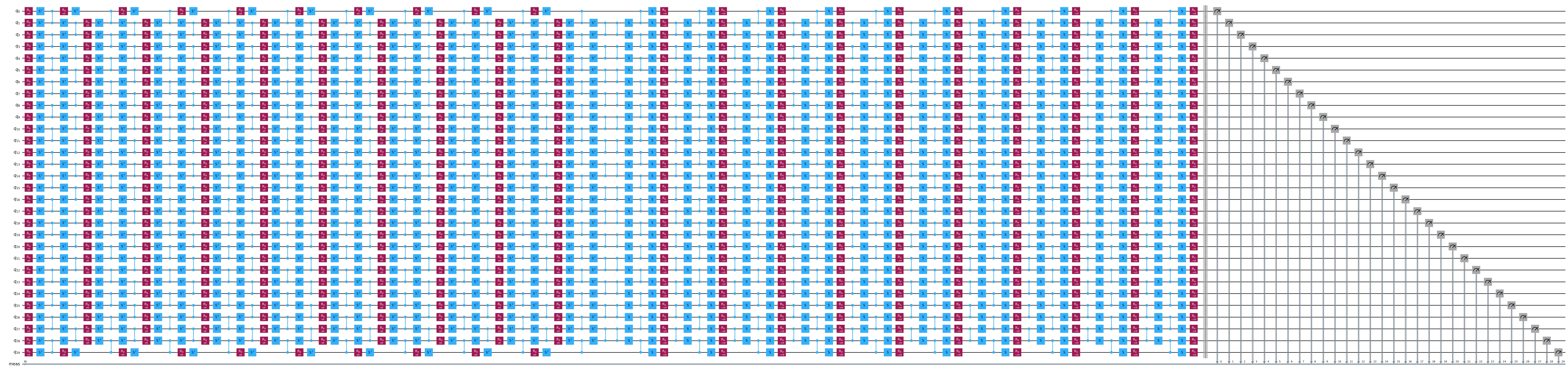
ตอนนี้เราจะรันขั้นตอนการทำงานของ PNA ทั้งหมดบนโมเดล kicked Ising ขนาด 30 site ที่รันบนฮาร์ดแวร์ IBM Quantum® ตามสี่ขั้นตอนของ Qiskit pattern
ขั้นตอนที่ 1: แปลงเป็นปัญหาควอนตัม
สร้าง Trotter circuit ที่ mirror และ observable
สำหรับการทดลองนี้ เราจะศึกษาพลวัตตามเวลาของโมเดล kicked Ising ขนาด 30 site บนสายโซ่สปิน 1D Hamiltonian ที่พิจารณาคือ:
,
โดยที่ อธิบายการเชื่อมโยงของสปินที่อยู่ใกล้เคียงกัน และสนามตามขวางที่กระทำทั่วทั้งระบบ (global) ถูกกำหนดเป็น ยิ่ง อยู่ห่างจากมุม Clifford มากเท่าไร (นั่นคือ ) ก็ยิ่งยากขึ้นที่จะแพร่กระจายตัวสร้าง anti-noise ผ่าน circuit
สำหรับการเลือก observable เราจะพิจารณา magnetization เฉลี่ยของ single-site โดยที่ คือจำนวน site
num_qubits = 30
num_trotter_steps = 10
rx_angle = np.pi / 8

# Avg single-site magnetization
id_pauli = Pauli("I" * num_qubits)
observable = (
    SparsePauliOp([id_pauli.dot(Pauli("Z"), [i]) for i in range(num_qubits)])
    / num_qubits
)

# Implement Trotterized kicked-Ising model
circuit = QuantumCircuit(num_qubits)
for _step in range(num_trotter_steps):
    circuit.rx(rx_angle, range(num_qubits))
    for first_qubit in (1, 2):
        for idx in range(first_qubit, num_qubits, 2):
            # equivalent to Rzz(-pi/2):
            circuit.sdg([idx - 1, idx])
            circuit.cz(idx - 1, idx)
# Append the inverse circuit to complete the mirroring
circuit.compose(circuit.inverse(), inplace=True)
circuit.measure_active()
circuit.draw("mpl", fold=-1)
ขั้นตอนที่ 2: เพิ่มประสิทธิภาพปัญหาสำหรับการรันบนฮาร์ดแวร์
ขั้นตอนถัดไปคือการเตรียม Trotter circuit ที่ mirror ของเราสำหรับการรันบนฮาร์ดแวร์ IBM Quantum จริง การรันบน QPU ต้องการมากกว่าแค่การสร้าง circuit เชิงนามธรรม เนื่องจากเราต้องเพิ่มประสิทธิภาพมันเพื่อให้:
-
สอดคล้องกับชุด gate เนทีฟและการเชื่อมต่อของ backend การ transpile จะแปลง circuit เชิงตรรกะเป็น ISA circuit ที่รองรับโดย backend เป้าหมาย สิ่งนี้ทำให้มั่นใจว่าทุก gate และปฏิสัมพันธ์ของ qubit สามารถทำได้จริงทางกายภาพ
-
เราสามารถระบุลักษณะของ noise ในระดับ circuit layer ได้ PNA อาศัยการเรียนรู้และเผยแพร่ inverse noise channel เพื่อทำสิ่งนี้อย่างมีประสิทธิภาพ เราแบ่ง circuit ที่ transpile แล้วออกเป็น two-qubit layer ที่ไม่ซ้ำกันซึ่งถูก "box" box เหล่านี้ช่วยให้เราสามารถเชื่อมโยงแต่ละ layer ของ circuit กับ noise model ที่เรียนรู้มาของมันเอง
-
เราสามารถป้อน noise model ที่สมจริงเข้าสู่ PNA ได้ เมื่อ circuit ถูก box แล้ว เราใช้บริการ
NoiseLearnerV3เพื่อเรียนรู้ Pauli noise channel ที่ส่งผลต่อแต่ละ two-qubit layer ที่ไม่ซ้ำกันในเชิงทดลอง จากนั้นโมเดลที่เรียนรู้เหล่านี้จะถูกเชื่อมโยงกลับไปยัง circuit ผ่านคำอธิบายประกอบของ Samplomatic
โดยรวมแล้ว ขั้นตอนนี้เชื่อมช่องว่างระหว่าง circuit ที่ mirror ในอุดมคติกับ circuit ที่พร้อมสำหรับฮาร์ดแวร์ที่มี noise model ที่เรียนรู้มา ด้วยการตั้งค่านี้ PNA สามารถแพร่กระจาย inverse noise channel ผ่าน circuit และปรับ observable ตามนั้นได้
เชื่อมต่อกับ backend และ transpile เป็น ISA circuit
ก่อนอื่นเราเริ่มต้น IBM Quantum Compute Service และเลือก backend ยืนยันตัวตนด้วยบัญชีของคุณเองโดยทำตาม คำแนะนำในการบันทึกข้อมูลรับรอง หลังจากนั้น QiskitRuntimeService() จะดึงข้อมูลเหล่านั้นมาใช้โดยอัตโนมัติ
# Initialize IBM Quantum Compute Service using your saved credentials
service = QiskitRuntimeService()

backend = service.least_busy(
    operational=True, simulator=False, min_num_qubits=num_qubits
)
# Re-fetch with fractional gates enabled (least_busy does not forward this)
# Fractional gates are enabled so the non-Clifford Rx rotations are supported natively.
backend = service.backend(backend.name, use_fractional_gates=True)
print(f"Selected backend: {backend.name}")
Selected backend: ibm_fez
ถัดไป เราเลือกสายโซ่ qubit ที่เชื่อมต่อกันบน backend และ transpile circuit ลงไป
โดยใช้ helper find_qubit_chain ที่กำหนดไว้ในส่วน Setup เราเลือกแนว qubit ทางกายภาพที่เชื่อมต่อกันจำนวน num_qubits จากนั้นเรา transpile ด้วย optimization_level=0 และตรึงสายโซ่นี้เป็น initial_layout ซึ่งรักษาโครงสร้าง layer ของ two-qubit-gate ของ circuit ที่ mirror ไว้อย่างแม่นยำ โครงสร้างนั้นคือสิ่งที่ขั้นตอนการ box และการเรียนรู้ noise ต้องอาศัย ดังนั้นจึงต้องหลีกเลี่ยงระดับการเพิ่มประสิทธิภาพที่สูงกว่า (ซึ่งจะยกเลิก gate ที่ mirror) ในที่นี้
# Find a connected, low-error chain of qubits on the chosen backend
layout = find_qubit_chain(backend, num_qubits)

# Transpile the circuit for the target backend, pinning the chain as the layout.
# optimization_level=0 preserves the mirrored two-qubit-gate layers that the
# boxing and noise-learning steps rely on.
pm = generate_preset_pass_manager(
    backend=backend, optimization_level=0, initial_layout=layout
)
isa_circuit = pm.run(circuit)
isa_observable = observable.apply_layout(isa_circuit.layout)
isa_circuit.draw("mpl", fold=-1)

Twirl two-qubit gate layer และการวัด และหา layer ที่ไม่ซ้ำกัน
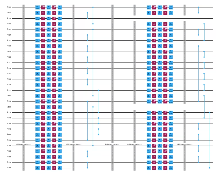
เราใช้ samplomatic เพื่อ box circuit และระบุ two-qubit layer ที่ไม่ซ้ำกัน box เป็นโครงสร้างที่จัดกลุ่มคำสั่งเข้าด้วยกัน เพื่อให้เจตนาหรือคำอธิบายประกอบเฉพาะสามารถนำไปใช้กับ gate ทั้งหมดภายใน box เดียวกันได้อย่างสม่ำเสมอในภายหลัง
ในที่นี้ เราเรียกใช้เมธอด generate_boxing_pass_manager ซึ่งทำมากกว่าการระบุ two-qubit layer เพียงอย่างเดียว โดยจะทำงานสำคัญหลายอย่าง:
-
จัดกลุ่ม two-qubit layer ทั้งหมดใน circuit
-
ใช้คำอธิบายประกอบ
TwirlและChangeBasisกับ layer เหล่านั้น -
จัดกลุ่มการดำเนินการวัดเข้าไปในส่วนที่ถูก box ของตัวเอง และ
-
ใช้คำอธิบายประกอบ
InjectNoiseกับแต่ละ two-qubit layer
คำอธิบายประกอบเหล่านี้กำหนดวิธีการจัดการ noise การเปลี่ยน basis และ twirling ตลอดทั้ง circuit นอกจากนี้ยังกำหนดโครงสร้างที่ใช้ในภายหลังสำหรับการเรียนรู้และลดข้อผิดพลาดของ noise
ตัวเลือกการกำหนดค่าหลักคือ:
-
enable_gates/enable_measures: True: box two-qubit gate layer ทั้งหมดและการวัดปลายทาง single-qubit gate จะถูกวาง left-dressed ไว้ภายใน box -
measure_annotations: all: รวมคำอธิบายประกอบTwirlและChangeBasisไว้ใน box การวัด -
twirling_strategy: active: twirl active qubit ทั้งหมดในแต่ละ box ที่มี entangling gate -
inject_noise_targets: gates: เพิ่มคำอธิบายประกอบInjectNoiseให้กับ box ที่มีคำอธิบายประกอบTwirlทั้งหมดที่มี entangling gate -
inject_noise_strategy: uniform_modification: ปรับสเกล noise layer ทั้งหมดอย่างเท่าเทียมกันทั่วทั้ง circuit
# Box up circuit with Twirl and InjectNoise annotations
pm = generate_boxing_pass_manager(
    enable_gates=True,
    enable_measures=True,
    measure_annotations="all",
    twirling_strategy="active",
    inject_noise_targets="gates",
    inject_noise_strategy="uniform_modification",
)
boxed_circuit = pm.run(isa_circuit)
draw_circ = QuantumCircuit(boxed_circuit.num_qubits)
draw_circ.append(boxed_circuit.data[0], qargs=boxed_circuit.data[0].qubits)
draw_circ.append(boxed_circuit.data[1], qargs=boxed_circuit.data[1].qubits)
draw_circ.draw("mpl", fold=-1, scale=0.3, idle_wires=False)

สร้าง template circuit และ samplex ซึ่งกำหนดวิธีการสุ่มตัวอย่าง circuit
ในที่นี้เรายังเพิ่มการวัด spectator และ post-selection ซึ่งจำเป็นสำหรับการทำ post-selection บนตัวอย่างผลลัพธ์จาก Executor
# Build template circuit and samplex for later use with the "Executor"
template_circuit, samplex = samplomatic.build(boxed_circuit)

# Add post-selection instructions to the template circuit
post_selection_pm = PassManager(
    [
        AddSpectatorMeasures(backend.coupling_map),
        AddPostSelectionMeasures(x_pulse_type="rx"),
    ]
)
template_circuit = post_selection_pm.run(template_circuit)
draw_circ = template_circuit.copy_empty_like()
draw_circ.data = template_circuit.data[:324]
draw_circ.draw("mpl", fold=-1, scale=0.3, idle_wires=False)
เรียนรู้ noise โดยใช้ NoiseLearnerV3
ก่อนที่เราจะใช้ PNA เพื่อลดข้อผิดพลาด เราต้องระบุลักษณะ noise ที่ส่งผลต่อแต่ละ two-qubit layer ที่ไม่ซ้ำกันและ measurement layer ใน circuit ของเราก่อน ในการทำเช่นนี้ เราใช้โปรแกรม NoiseLearnerV3 เพื่อเรียนรู้ noise model ในเชิงทดลองสำหรับแต่ละ layer ที่ระบุไว้ก่อนหน้านี้ learner จะทำการทดลองสไตล์ benchmarking ที่ประมาณ noise channel ที่ส่งผลต่อแต่ละ layer และส่งคืนอ็อบเจกต์ผลลัพธ์ที่มีโมเดลที่เรียนรู้มา
เราเริ่มด้วยการระบุ layer ที่ไม่ซ้ำกันใน circuit ของเราโดยใช้ find_unique_box_instructions จาก samplomatic สิ่งนี้ทำให้มั่นใจว่าเราจะเรียนรู้ noise เพียงครั้งเดียวต่อประเภท layer ที่แตกต่างกัน ซึ่งลดจำนวนการทดลองและต้นทุนช็อตทั้งหมด รายการ layer ที่ได้จะถูกส่งไปยัง noise learner
มีพารามิเตอร์สำคัญสองสามตัวที่ควบคุมวิธีการเรียนรู้ noise:
-
num_randomizations: จำนวน circuit สุ่มที่ใช้ต่อการกำหนดค่าการเรียนรู้ -
shots_per_randomization: จำนวนช็อตที่ใช้ต่อ circuit การเรียนรู้แบบสุ่ม -
layer_pair_depths: ความลึกของ circuit (วัดเป็นจำนวนคู่) ที่ใช้ในการทดลองการเรียนรู้ -
post_selection: เปิดใช้งาน post-selection แบบ edge-based โดยใช้ gaterxเพื่อใช้พัลส์หลังการวัด
# Noise learning parameters
num_randomizations_nl = 64
shots_per_randomization_nl = 128

# Match the deepest noise-learning depth to the depth of the circuit being
# mitigated. ``layer_pair_depths`` are measured in layer pairs (a layer + its
# inverse), so the deepest value is half the circuits's two-qubit-layer depth.
# Learning to this depth improves the quality of the mitigation.

depth_2q = isa_circuit.depth(lambda instr: instr.operation.num_qubits == 2)
max_layer_pair_depth = depth_2q // 2

# Use a fixed schedule of learning depths, but drop any that exceed the circuit's
# depth and always cap the deepest value at ``max_layer_pair_depth`` so we never
# learn deeper than the circuit being mitigated
candidate_depths = [1, 2, 4, 8, 12, 16, 24, 32, 40, 48]
layer_pair_depths = sorted(
    {d for d in candidate_depths if d < max_layer_pair_depth}
    | {max_layer_pair_depth}
)

# Find the unique instructions (layers) from the boxed-up circuit
unique_2q_layers_and_meas = find_unique_box_instructions(
    boxed_circuit, normalize_annotations=None, undress_boxes=True
)

# Configure and run the noise learner on the unique layers.
# Options can be passed directly as a dictionary.
noise_learner_options = {
    "num_randomizations": num_randomizations_nl,
    "shots_per_randomization": shots_per_randomization_nl,
    "layer_pair_depths": layer_pair_depths,
    "post_selection": {
        "enable": True,
        "strategy": "edge",
        "x_pulse_type": "rx",
    },
    "environment": {"job_tags": ["TUT_PNA"]},
}

noise_learner = NoiseLearnerV3(backend, noise_learner_options)
noise_learner_job = noise_learner.run(unique_2q_layers_and_meas)
noise_learner_result = noise_learner_job.result()
แสดงภาพอัตรา noise ที่เรียนรู้มา
หลังจากเรียนรู้ noise model แล้ว เราสามารถตรวจสอบการกระจายของอัตราข้อผิดพลาดที่อนุมานได้สำหรับทั้งการดำเนินการแบบ one-qubit และ two-qubit โค้ดด้านล่างดึงการแทนค่าแบบ Pauli-Lindblad จากผลลัพธ์ noise ที่เรียนรู้มาและรวบรวมอัตรา noise ที่สอดคล้องกัน
สำหรับแต่ละ layer ที่เรียนรู้:
- เราแปลง noise model เป็นรายการแบบ sparse ของทูเพิล
(pstr, qubits, rate)โดยที่pstrคือ Pauli string ที่กระทำกับ qubit ที่กำหนด และrateคืออัตราข้อผิดพลาดที่เกี่ยวข้อง - เราแยกอัตราออกเป็นเทอมแบบ one-qubit (
len(pstr) == 1) และ two-qubit (len(pstr) == 2) - จากนั้นรายการอัตราจะถูกเรียงลำดับ และคำนวณค่ามัธยฐานของมัน
เราพล็อตการกระจายอัตรา noise แบบ one-qubit (สีแดง) และ two-qubit (สีน้ำเงิน) บนสเกลลอการิทึม โดยมีค่ามัธยฐานทำเครื่องหมายด้วยเส้นแนวตั้ง เพื่อให้เราสามารถเปรียบเทียบขนาดสัมพัทธ์ของตัวสร้าง Pauli-Lindblad ที่เรียนรู้มาได้ ลำดับของอัตรา one-qubit และ two-qubit ขึ้นอยู่กับอุปกรณ์และ layer เฉพาะที่ถูกระบุลักษณะ ในการรันนี้ ตัวสร้าง single-qubit (weight-1) มีอัตรามัธยฐานที่มากกว่า
hw_rates_1q = []
hw_rates_2q = []
for nlr in noise_learner_result[:2]:
    plm_list = nlr.to_pauli_lindblad_map().to_sparse_list()
    hw_rates_1q += [
        rate for (pstr, qubits, rate) in plm_list if len(pstr) == 1
    ]
    hw_rates_2q += [
        rate for (pstr, qubits, rate) in plm_list if len(pstr) == 2
    ]
hw_rates_1q = sorted(hw_rates_1q)
hw_rates_2q = sorted(hw_rates_2q)
median_1q = hw_rates_1q[len(hw_rates_1q) // 2]
median_2q = hw_rates_2q[len(hw_rates_2q) // 2]
fig, ax = plt.subplots(1, 1, figsize=(14, 5))
ax.scatter(
    (hw_rates_1q),
    [(i) / (len(hw_rates_1q) - 1) for i in range(len(hw_rates_1q))],
    color="red",
    label="1q rates",
)
ax.set_xscale("log")
ax.set_ylim(0, 1.1)
ax.vlines(median_1q, 0, 1, color="red")
ax.text(median_1q * 1.1, 0.1, f"{median_1q:.2e}")
ax.scatter(
    (hw_rates_2q),
    [(i) / (len(hw_rates_2q) - 1) for i in range(len(hw_rates_2q))],
    color="blue",
    label="2q rates",
)
ax.set_xscale("log")
ax.set_ylim(0, 1.1)
ax.vlines(median_2q, 0, 1, color="blue")
ax.text(median_2q * 1.1, 0.2, f"{median_2q:.2e}")
ax.set_title("Learned noise rates")
ax.set_xlabel("Noise rate")
ax.set_yticks([])
plt.legend()
<matplotlib.legend.Legend at 0x125336120>

เชื่อมโยง circuit box กับ noise ที่เรียนรู้มา
เมื่อเราได้ noise model สำหรับแต่ละ two-qubit layer ที่ไม่ซ้ำกันแล้ว เราจำเป็นต้องเชื่อมโยงกับคำอธิบายประกอบ InjectNoise ที่สอดคล้องกันภายใน circuit ที่ถูก box
คำสั่ง InjectNoise เป็นคำอธิบายประกอบของ samplomatic ที่ใช้ single-qubit dresser เพื่อฉีด noise เข้าไปใน circuit ในลักษณะที่ควบคุมและกำหนดค่าได้ มันช่วยให้สามารถจำลอง noise แบบโมดูลาร์ในหลาย layer ได้
คำอธิบายประกอบ InjectNoise แต่ละอันประกอบด้วย:
InjectNoise.ref- ตัวระบุที่ไม่ซ้ำกันสำหรับคำอธิบายประกอบ ใช้โดยอ็อบเจกต์samplexเพื่อกำหนด noise model ที่สอดคล้องกันอย่างถูกต้องInjectNoise.modifier_ref(ตัวเลือกเสริม) - การอ้างอิงรองที่อนุญาตให้ปรับสเกล noise model ที่กำหนดด้วยตัวคูณ
ในขั้นตอนนี้ เราสร้างการจับคู่จาก InjectNoise.ref แต่ละอันไปยัง noise model ที่เรียนรู้มาที่สอดคล้องกัน (PauliLindbladMap) การจับคู่นี้ทำให้มั่นใจว่าแต่ละ entangling gate layer ใน circuit จับคู่กับ noise model ที่เหมาะสม เพื่อให้ผลกระทบของ noise ถูกนำไปใช้อย่างแม่นยำในระหว่างการสุ่มตัวอย่างและขั้นตอนการลด noise ที่ตามมา
# map inject noise refs to pauli lindblad maps
refs_to_noise_models = {}
for instruction, result in zip(
    unique_2q_layers_and_meas, noise_learner_result, strict=False
):
    if inject_noise_annot := get_annotation(
        instruction.operation, InjectNoise
    ):
        refs_to_noise_models[inject_noise_annot.ref] = (
            result.to_pauli_lindblad_map()
        )
แพร่กระจาย observable ผ่าน anti-noise ที่เรียนรู้มา
ตามที่ได้กล่าวไปข้างต้น ขั้นตอนนี้ทำเป็นสองขั้น ขั้นแรก เรา propagate anti-noise generator ไปยังจุดสิ้นสุดของ Circuit หลังจากนั้น เรา propagate observable ผ่าน generator ที่วิวัฒน์แล้วนั้น กระบวนการนี้ทำซ้ำสำหรับ anti-noise generator แต่ละตัวใน Circuit ในการนำไปใช้งานนี้ generator แต่ละตัวใน layer ที่กำหนดจะถูก propagate ไปยังจุดสิ้นสุดของ Circuit แบบขนาน นอกจากนี้ยังใช้ Python multiprocessing เพื่อทำการ forward-propagation ของ anti-noise และการ back-propagation ของ observable แบบขนานไปพร้อมกัน วิธีนี้ช่วยป้องกันการสะสมของ generator ที่วิวัฒน์แล้วในหน่วยความจำ และยังใช้ทรัพยากรการประมวลผลได้อย่างเต็มที่ด้วย
เมื่อรัน PNA คุณต้องให้ noisy circuit และ observable เสมอ ถ้า noisy circuit ของคุณเป็น boxed circuit ที่มี annotation แบบ InjectNoise คุณต้องให้ mapping ที่เราสร้างไว้ในขั้นตอนก่อนหน้า นอกจากนี้ยังสามารถส่ง circuit ที่ไม่ใช่ boxed ซึ่งมีคำสั่ง PauliLindbladError จาก qiskit-aer ได้ ในกรณีนั้น ไม่จำเป็นต้องให้ refs_to_noise_models นอกจากอินพุตหลักแล้ว ให้พิจารณาสิ่งต่อไปนี้ด้วย:
-
max_err_terms: จำนวนเทอมที่จะเก็บไว้ใน anti-noise generator แต่ละตัวขณะที่มันถูก forward-propagate โดยทั่วไปการเพิ่มค่านี้จะช่วยเพิ่มความแม่นยำ แต่พฤติกรรมนี้ไม่รับประกันว่าจะเป็นแบบ monotonic -
max_obs_terms: จำนวนเทอมที่จะเก็บไว้ใน noise-mitigating observable, ขณะที่มันถูก back-propagate ผ่าน anti-noise ที่วิวัฒน์แล้ว โดยทั่วไปค่าที่มากขึ้นจะเพิ่มความแม่นยำ แต่ไม่รับประกันว่าจะเป็นแบบ monotonic -
num_processes: จำนวนคอร์ที่จะจัดสรรให้กับกระบวนการนี้ อย่าลืมว่า generator จะถูก forward-propagate และนำไปใช้กับ observable แบบขนาน -
search_step: ขั้นตอน back-propagation ใช้วิธี greedy เพื่อประมาณค่า conjugate ของตัวดำเนินการสองตัวใน Pauli basis วิธีนี้สามารถทำให้เร็วขึ้นได้โดยเพิ่มค่าsearch_stepดูข้อมูลเพิ่มเติมได้ที่ เอกสารpauli-prop -
num_to_measure: แม้ว่าตัวแปรนี้จะไม่ใช่อินพุตของgenerate_noise_mitigating_observableแต่เราใช้มันเพื่อควบคุมว่าเราต้องการวัดเทอมกี่เทอมจาก ในที่นี้เราวัดเพียง 30 เทอมสูงสุด ซึ่งเป็นเทอมดั้งเดิมใน observable ของเรา เทอมเหล่านี้ถูกปรับสเกลใหม่แล้วเพื่อให้การวัดเทอมเหล่านั้นมีผลในการลด gate noise ที่เรียนรู้มา แม้ว่าเราจะวัดเพียง 30 เทอมจาก แต่ก็ยังมีประโยชน์ที่จะปล่อยให้มันเติบโตขึ้น เนื่องจากจะเพิ่มความแม่นยำของค่าปัจจัยการปรับสเกลของเทอมชั้นนำ
# PNA parameters
num_processes = 8
max_err_terms = 10_000
max_obs_terms = 10_000
num_to_measure = num_qubits

obs_tilde_isa = generate_noise_mitigating_observable(
    boxed_circuit,
    isa_observable,
    refs_to_noise_models,
    max_err_terms=max_err_terms,
    max_obs_terms=max_obs_terms,
    num_processes=num_processes,
    print_progress=True,
    search_step=8,
)
p_2_v = {p: v for v, p in enumerate(layout)}
obs_tilde_virtual = SparsePauliOp.from_sparse_list(
    [
        (pstr, [p_2_v[p] for p in p_qubits], coeff)
        for (pstr, p_qubits, coeff) in obs_tilde_isa.to_sparse_list()
    ],
    num_qubits=num_qubits,
)
obs_tilde_virtual = obs_tilde_virtual[
    np.argsort(np.abs(obs_tilde_virtual.coeffs))[::-1]
][:num_to_measure]
Finished! 13740 / 13740 generators propagated.
obs_tilde_isa = obs_tilde_isa[np.argsort(np.abs(obs_tilde_isa.coeffs))][::-1]
plt.xscale("log")
plt.yscale("log")
plt.title(r"$\tilde{O}$ coeff magnitudes")
plt.ylabel("Magnitude")
plt.xlabel("Pauli term index")
plt.plot(np.abs(obs_tilde_isa.coeffs), ".")
[<matplotlib.lines.Line2D at 0x124b0a120>]

แปลง measurement bases ให้เป็นรูปแบบมาตรฐาน
ต่อไป เราจะหาชุดของ bases ขั้นต่ำที่จะวัด เพื่อให้ครอบคลุมทุกเทอม Pauli ใน observable ที่วัด (observable หลายตัวอาจถูกวัดพร้อมกันได้หาก commute แบบ qubit-wise) เนื่องจากเราวัดเฉพาะเทอมใน observable ดั้งเดิมของเรา ซึ่งเป็นผลรวมของ Pauli แบบ single-Z ทั้งหมด จึงต้องการเพียง basis เดียว: all-Z basis
นอกจากการหาชุดของ Pauli measurement bases แล้ว เรายังต้อง map เทอม Pauli เหล่านี้ให้เป็นรูปแบบมาตรฐานที่ Executor คาดหวัง สำหรับข้อมูลเพิ่มเติมเกี่ยวกับการเรียงลำดับ qubit แบบมาตรฐาน โปรดดู เอกสาร Samplomatic
meas_box = boxed_circuit.data[-1]
canonical_qubits = [
    idx
    for idx, qubit in enumerate(boxed_circuit.qubits)
    if qubit in meas_box.qubits
]
c_2_p = {
    c: p for c, p in enumerate(canonical_qubits)
}  # canonical -> physical
p_2_v = {p: v for v, p in enumerate(layout)}  # physical -> virtual
c_2_v = {c: p_2_v[p] for c, p in c_2_p.items()}  # canonical -> virtual
meas_bases, bases_reverser = get_measurement_bases(obs_tilde_virtual)
meas_bases_canonical = [
    np.array([base[c_2_v[c]] for c in range(num_qubits)], dtype=np.uint8)
    for base in meas_bases
]
ขั้นตอนที่ 3: รันการทดลองควอนตัม
ระบุวิธีการ sample ใน QuantumProgram
ตอนนี้เราจะตั้งค่า QuantumProgram ซึ่งทำหน้าที่เป็นที่เก็บส่วนกลางสำหรับ Circuit และการตั้งค่าการ sample ทั้งหมดที่จะถูกรันโดย Executor ออบเจ็กต์นี้กำหนดว่าอินสแตนซ์ Circuit แบบสุ่มจะถูกสร้าง, จัดกลุ่ม, และรันอย่างไร เพื่อสร้างผลลัพธ์การวัดที่ใช้ใน PNA
QuantumProgram สามารถมีหลายรายการ แต่ละรายการประกอบด้วย template circuit และออบเจ็กต์ samplex ที่สอดคล้องกัน ซึ่งกำหนดว่าการสุ่มจะถูกนำมาใช้อย่างไร แนวคิดเชิงนามธรรมนี้ทำให้ Executor สามารถจัดการขั้นตอนการทำงานทั้งหมดเป็นโปรแกรมเดียวที่เป็นโมดูล — ตั้งแต่การสร้าง Circuit แบบสุ่มไปจนถึงการเก็บและรวม shot
ในขั้นตอนนี้ เราจะสร้าง QuantumProgram ที่รันการทดลอง PNA ของเราโดยใช้ template circuit และ samplex ที่เราสร้างไว้ก่อนหน้านี้ การตั้งค่านี้ประกอบด้วยองค์ประกอบต่อไปนี้:
-
template_circuit: Circuit ที่มี gate ทั้งหมดที่จำเป็นในการทำให้เกิดการสุ่มที่ต้องการทั้งหมด (จากการ twirling randomization, พารามิเตอร์ ฯลฯ) -
samplex: ออบเจ็กต์ที่กำหนดการกระจายความน่าจะเป็นของ Circuit แบบสุ่มที่เป็นไปได้ทั้งหมดที่จะใช้ในการ sample -
samplex_arguments: การ bind ที่จำเป็นในการกำหนดsamplexอย่างสมบูรณ์-
basis_changes: นี่คือจุดที่เราระบุชุดของ bases ที่จะวัด ซึ่งจะครอบคลุมเทอม Pauli ทั้งหมดใน observable ที่วัด -
noise_scales.ref: เรากำหนดสเกลของแต่ละ noise layer เป็น0.0เพื่อป้องกันไม่ให้มี noise เพิ่มเติมถูกฉีดเข้าไปในตัวอย่างของเรา -
pauli_lindblad_maps: จำเป็นต้องมีหากnoise_scalesถูกส่งเข้ามา นี่เป็นเพียงการ map noise layer ไปยัง noise model ที่เกี่ยวข้อง
-
-
shape: tuple ของ shape ที่ใช้ขยาย shape โดยนัยที่กำหนดโดยsamplex_argumentsแกนที่มีขนาดมากกว่า 1 ซึ่งเกิดจากการขยายนี้ จะเป็นตัวแจกแจงจำนวน randomization
# Control the # of shots during execution
shots_per_randomization_exec = 64
num_randomizations_exec = 6144

# Zero out the noise to prevent noise from being injected during execution.
# We only added InjectNoise annotations so PNA could associate the noise
# to layers in the circuit
samplex_inputs = {f"noise_scales.{ref}": 0.0 for ref in refs_to_noise_models}
samplex_inputs |= {"pauli_lindblad_maps": refs_to_noise_models}

# Specify the bases to measure. The samplex exposes one basis-change input per
# ChangeBasis-annotated box; here a single all-Z basis covers every term. We
# look up the basis-change interface name rather than hardcoding an index, since
# the name depends on the circuit's box structure.
bases_broadcastable = np.expand_dims(np.array(meas_bases_canonical), axis=1)
samplex_inputs |= {
    spec.name: bases_broadcastable
    for spec in samplex.inputs().get_specs(r"^basis_changes\.")
}

# Convert samplex_inputs into a dict to pass to QuantumProgram
samplex_arguments = (
    samplex.inputs().make_broadcastable().bind(**samplex_inputs)
)

# Instantiate the QuantumProgram with the specified parameters
program = QuantumProgram(shots=shots_per_randomization_exec)
program.append_samplex_item(
    circuit=template_circuit,
    samplex=samplex,
    samplex_arguments=samplex_arguments,
    shape=(num_randomizations_exec,),
)
Sample Circuit โดยใช้ Executor
เมื่อเรากำหนด QuantumProgram แล้ว การรันการทดลองก็ทำได้ง่ายมาก เราเพียงแค่สร้างอินสแตนซ์ของออบเจ็กต์ Executor ให้ backend แก่มัน และรันโปรแกรม
# Execute (sample) the circuit
executor = Executor(backend)
job_exec = executor.run(program)
exec_results = job_exec.result()
ขั้นตอนที่ 4: สร้างใหม่และวิเคราะห์ผลลัพธ์
ในการคำนวณค่าคาดหวังที่ลดข้อผิดพลาดแล้ว เราทำสิ่งต่อไปนี้:
-
คำนวณปัจจัยการปรับสเกล TREX โดยอิงจาก noise ที่เรียนรู้มาซึ่งส่งผลต่อการวัด
-
สร้าง mask เพื่อเก็บเฉพาะตัวอย่างที่ผ่านการ post-select และ
-
ใช้ฟังก์ชัน
executor_expectation_valuesจากqiskit-addon-utilsเพื่อรวมข้อมูลทั้งหมดเข้าเป็นค่าคาดหวังที่ลดข้อผิดพลาดแล้ว
# Computing the TREX factors
measurement_noise_map = noise_learner_result[2].to_pauli_lindblad_map()
trex_rescale_factors = trex_factors(measurement_noise_map, bases_reverser)

# Post-select the results
post_selector = PostSelector.from_circuit(
    circuit=template_circuit, coupling_map=backend.coupling_map
)

# Compute the ps mask for filtering results
mask = post_selector.compute_mask(exec_results[0], strategy="edge")

# Compute expvals using post selected results
results = executor_expectation_values(
    exec_results[0]["meas"],
    bases_reverser,
    meas_basis_axis=0,
    avg_axis=1,
    measurement_flips=exec_results[0]["measurement_flips.meas"],
    pauli_signs=exec_results[0].get("pauli_signs", None),
    postselect_mask=mask,
    rescale_factors=trex_rescale_factors,
)
เปรียบเทียบกลยุทธ์การลดข้อผิดพลาด: PNA, PNA+TREX, PNA+PS, PNA+PS+TREX
เราคำนวณและแสดงภาพค่าคาดหวังสำหรับกลยุทธ์การลดข้อผิดพลาดหลายแบบโดยใช้ผลลัพธ์จาก Executor
bases_reverser_unmit = {Pauli("Z" * num_qubits): [observable]}
args = [
    (bases_reverser_unmit, None, None),
    (bases_reverser, None, None),
    (bases_reverser, None, trex_rescale_factors),
    (bases_reverser, mask, None),
    (bases_reverser, mask, trex_rescale_factors),
]

evs = []
for reverser, postsel_mask, factors in args:
    # Compute expvals using post selected results
    res_ps = executor_expectation_values(
        exec_results[0]["meas"],
        reverser,
        meas_basis_axis=0,
        avg_axis=1,
        measurement_flips=exec_results[0]["measurement_flips.meas"],
        pauli_signs=exec_results[0].get("pauli_signs", None),
        postselect_mask=postsel_mask,
        rescale_factors=factors,
    )
    res_ps = np.array(res_ps)
    evs.append(res_ps[:, 0][0])

experiments = ["PNA", "PNA+TREX", "PNA+PS", "PNA+PS+TREX"]
colors = ["#d9d9d9", "#b0b0b0", "#7f7f7f", "#4c4c4c"]
plt.bar(experiments, evs[1:], color=colors)
plt.axhline(y=1, color="green", linestyle="--", linewidth=2, label="Ideal")
plt.axhline(
    y=evs[0], color="red", linestyle="--", linewidth=2, label="Unmitigated"
)
plt.ylabel("Expectation value", fontsize=14)

plt.title(
    r"30q Mirrored Ising, 10 Trotter steps, $\theta_{rx}=\frac{\pi}{8}$",
    fontsize=14,
)
plt.legend(loc="upper left", bbox_to_anchor=(1.05, 1), borderaxespad=0.0)
plt.xticks(rotation=45)
plt.tight_layout()
plt.show()

ผลลัพธ์แสดงให้เห็นถึงประโยชน์สะสมของการรวมเทคนิคการลดข้อผิดพลาดต่างๆ เข้าด้วยกัน วิธี PNA แบบธรรมดาสามารถคืนค่าคาดหวังให้ใกล้เคียงกับค่าอ้างอิงในอุดมคติได้แล้ว ซึ่งบ่งชี้ว่าการแพร่กระจาย inverse noise channel เข้าไปใน observable ช่วยชดเชยข้อผิดพลาดของ two-qubit gate ได้อย่างมีประสิทธิภาพ
-
การเพิ่มการปรับน้ำหนักด้วย TREX (PNA+TREX) ช่วยปรับปรุงค่าประมาณเล็กน้อยโดยแก้ไขความไม่สมดุลในการ sampling ของ Circuit แบบสุ่ม
-
การ post-selection (PNA+PS) ให้การปรับปรุงที่เห็นได้ชัดเจนยิ่งขึ้น โดยการกรองผลการวัดที่ไม่สอดคล้องกันซึ่งน่าจะเกิดจาก error ที่หลงเหลืออยู่
-
สุดท้าย การรวมทั้งสองอย่างเข้าด้วยกัน (PNA+PS+TREX) ให้ผลลัพธ์ที่แม่นยำที่สุด เกือบตรงกับค่าในอุดมคติ แสดงให้เห็นว่ากลยุทธ์การลดข้อผิดพลาดเหล่านี้เสริมกันอย่างไร
โดยรวมแล้ว การเปรียบเทียบนี้เน้นให้เห็นว่า PNA เป็นรากฐานที่แข็งแกร่งสำหรับการประมาณค่าคาดหวังที่คำนึงถึง noise ในขณะที่ TREX และ post-selection มอบการปรับปรุงเพิ่มเติมที่ส่งเสริมกันเพื่อเพิ่มความแม่นยำต่อไป
ขั้นตอนถัดไป
หากคุณสนใจเนื้อหานี้ คุณอาจสนใจเนื้อหาต่อไปนี้ด้วย: