Probabilistic error cancellation ด้วย shaded lightcone
ประมาณการใช้งาน: 10 นาทีบนโปรเซสเซอร์ Heron (หมายเหตุ: นี่เป็นเพียงการประมาณการเท่านั้น เวลาการรันจริงของคุณอาจแตกต่างออกไป)
ผลลัพธ์การเรียนรู้
-
probabilistic error cancellation (PEC) คืออะไร และเหตุใด overhead ของการสุ่มตัวอย่าง จึงเติบโตแบบ exponential ตาม noise ทั้งหมดที่กระทำต่อ circuit
-
shaded lightcone (SLC) จำกัดขอบเขตของผลกระทบของแต่ละ noise term ต่อ observable เป้าหมายได้อย่างไร เพื่อให้คุณใช้งบประมาณการลด error ได้ตรงจุด — และวิธีที่ นอกเหนือจากการลด overhead แบบ zero-bias ที่ pure geometric lightcone ให้ไว้แล้ว การ shading ช่วยให้คุณแลก residual bias ที่มีขอบเขตกำกับเพื่อลด overhead การสุ่มตัวอย่างให้ต่ำลงไปอีก
-
วิธีเรียนรู้ layer noise ด้วย
NoiseLearnerV3และฉีด anti-noise ผ่านsamplomaticและ primitiveExecutor -
วิธีผสาน PEC และ PEC+SLC เข้ากับ TREX และ postselection เพื่อประมาณค่า expectation value บนฮาร์ดแวร์
ข้อกำหนดเบื้องต้น
-
ขั้นตอนการทำงานของ Qiskit patterns
-
การใช้ primitive Estimator เพื่อคำนวณ expectation value ของ observable
-
เทคนิคการลด error เช่น Pauli twirling และ TREX ที่กล่าวถึงใน ผสานตัวเลือกการลด error เข้ากับ primitive Estimator
ความเป็นมา
บทช่วยสอนนี้สาธิตวิธีลด error โดยใช้ addon shaded lightcone (SLC) addon นี้เป็นวิวัฒนาการของ เทคนิค probabilistic error cancellation (PEC) ซึ่งผู้ใช้จะเรียนรู้ noise ของ layer ที่ไม่ซ้ำกันในวงจร แล้วหักล้าง noise นั้นโดยการใช้ single-qubit gate และเทคนิคการประมวลผลภายหลัง เมื่อเทียบกับวิธีอื่น PEC ให้ขอบเขตที่แข็งแกร่งกว่าต่อ bias ของผลลัพธ์ที่ถูกลด error แต่มักมี overhead ที่สูงกว่าในแง่ของเวลาใช้ QPU ระหว่างทำ PEC เพื่อชดเชยการลดทอนของ expectation value จาก noise ผลลัพธ์เฉลี่ยจะถูกปรับสเกลด้วยตัวประกอบ โดยที่ คืออัตรา noise ที่เรียนรู้ได้ของ error Pauli ที่ layer ในวงจร การปรับสเกลนี้เพิ่ม variance ด้วยตัวประกอบ และด้วยเหตุนี้จึงคูณจำนวนการรันวงจรที่จำเป็นบน QPU ด้วย ซึ่งเราเรียกว่า sampling cost หรือ sampling overhead เนื่องจาก เติบโตแบบ exponential PEC จึงมักถูกจำกัดให้ใช้กับวงจรที่ตื้นหรือมี qubit น้อย เรียนรู้เพิ่มเติมเกี่ยวกับ PEC ได้ใน Probabilistic error cancellation with sparse Pauli-Lindblad models on noisy quantum processors
หากเราสามารถระบุ error ที่ไม่จำเป็นต้องถูกลดได้ เราก็สามารถลด sampling cost นี้ลงแบบ exponential ได้ ขั้นตอนแรกในทิศทางนี้คือการนำ locally-aware error mitigation มาใช้ ซึ่งใช้ "lightcone" แบบดั้งเดิมที่คำนวณได้อย่างรวดเร็วเพื่อลด PEC overhead โดยจำกัดขอบเขตความไวของ observable ต่อ error ตลอดทั้งวงจร ซึ่งขยายความเป็นไปได้ในการใช้ PEC กับปัญหาขนาดใหญ่ขึ้นในบางกรณี error ที่อยู่นอก lightcone นี้ไม่สามารถส่งผลต่อผลลัพธ์ที่วัดได้ จึงสามารถตัดออกจากขั้นตอนการหักล้าง error ได้ การตัดออกนี้ลด sampling overhead ซึ่งในบางกรณีลดลงอย่างมาก โดยไม่เพิ่ม bias เพิ่มเติม โดยเฉพาะอย่างยิ่ง สำหรับการวัด local observable ของวงจรที่มีความลึกคงที่ sampling overhead ที่จำเป็นในที่สุดจะอิ่มตัวเมื่อขยายจำนวน qubit ในวงจร (ดู Fig. 2b ใน Locality and error mitigation of quantum circuits)
Shaded lightcone (SLC) ก้าวไปไกลกว่านั้น โดยใช้การจำลองแบบคลาสสิกเพื่อจำกัดขอบเขตความไวต่อ error ตลอดทั้งวงจรให้แน่นยิ่งขึ้น สิ่งนี้แลกเวลาใช้ QPU บางส่วนกับเวลาใช้ CPU และลด sampling overhead ที่จำเป็นในการปรับ normalize bias แทนที่จะใช้จุดตัดแบบเข้ม (hard cutoff) error ที่เป็นไปได้แต่ละตัวในวงจรจะถูกกำหนด "เฉด (shade)" แบบไล่ระดับที่จำกัดขอบเขตบนของความไวของ expectation value ของ observable ต่อ error นั้น (สำหรับขอบเขตแบบ backward-propagated ที่นำเสนอด้านล่าง ความไวนี้ยังขึ้นอยู่กับ initial state ของวงจร ด้วย — ซึ่งคือ all-zero state ในขั้นตอนการทำงานทั่วไปและในบทช่วยสอนนี้) การกำหนดลักษณะเฉพาะที่ปรับปรุงนี้ช่วยให้สามารถประยุกต์ใช้ PEC ได้อย่างมีประสิทธิภาพและตรงเป้าหมายมากขึ้น โดยมี variance ลดลง ในขณะเดียวกันก็ให้ผู้ใช้สามารถควบคุมปรับ bias ในการประมาณค่า observable ได้ ดู Lightcone shading for classically accelerated quantum error mitigation สำหรับรายละเอียดเพิ่มเติม
ขั้นตอนการทำงานของเราสำหรับ SLC addon ใช้ไลบรารี samplomatic ร่วมกับคลาส QuantumProgram และ Executor ที่ถูกเพิ่มเข้าไปใน Qiskit Runtime ใน qiskit-ibm-runtime v0.47.0 ซึ่งช่วยให้ผู้ใช้สามารถควบคุมการตั้งค่าการรันได้อย่างเป็นโมดูลมากขึ้นสำหรับการระงับและลด error ในขณะที่ยังคงความง่ายในการใช้งาน อ่านเพิ่มเติมได้ในคู่มือ directed execution model
ภาพรวมขั้นตอนการลด error ของ SLC โดยสังเขป
สำหรับการจำลอง noise ของ QPU เราใช้ sparse Pauli-Lindblad noise model ที่มีอัตรา error ของ Pauli แบบ one- และ two-qubit ซึ่งสร้างขึ้นในระดับท้องถิ่นบน qubit และ edge แต่ละอันของอุปกรณ์ ด้วยทางเลือกนี้ ขั้นตอนการลด error ของ SLC ที่นำเสนอในบทช่วยสอนนี้มีดังนี้:
a. CPU — จำกัดขอบเขตผลกระทบต่อ error ของ one- และ two-qubit Pauli error
-
Forward propagation (จำกัดขอบเขตผลกระทบต่อ observable) แพร่กระจาย error แต่ละตัวไปยังจุดสิ้นสุดของวงจรและคำนวณ commutator กับ observable
-
ตัด operator term ระหว่างการวิวัฒนาการเพื่อให้การคำนวณสามารถจัดการได้
-
จำกัดขอบเขตเหล่านี้ให้แน่นยิ่งขึ้นด้วย back-propagation แบบหลวมของ observable โดยอิงจาก quantum speed limit
-
-
Backward propagation (จำกัดขอบเขตผลกระทบต่อ initial state) แพร่กระจาย error แต่ละตัวไปยังจุดเริ่มต้นของวงจรและคำนวณ commutator กับ initial state
b. QPU — เรียนรู้อัตรา noise ใช้ NoiseLearnerV3 เพื่อประมาณอัตราของ Pauli-Lindblad noise model
c. CPU — จัดลำดับความสำคัญการลด error
-
อัปเดตขอบเขตที่รวมกันด้วยอัตรา noise ที่เรียนรู้แล้ว รวมขอบเขตแบบ forward และ backward ที่คำนวณไว้ก่อนหน้านี้ และอัปเดตด้วยอัตรา noise ที่เรียนรู้แล้ว
-
จัดอันดับองค์ประกอบ noise ที่จะลดโดยใช้ขอบเขตที่คำนวณและอัตราที่เรียนรู้แล้ว จัดลำดับความสำคัญของ noise error ที่เป็นไปได้แต่ละตัวตามผลกระทบที่ประมาณการได้ต่อ bias และค่าใช้จ่ายที่เกี่ยวข้องในการแก้ไข
d. QPU — แทรก anti-noise และรัน รันวงจรที่สนใจด้วย anti-noise (noise ผกผัน) ที่ระบุโดยใช้ annotation Box
e. CPU — ประมาณค่า observable คำนวณ expectation value โดยใช้ post-selection ที่อิงตามการวัดเพื่อลดผลกระทบของ noise แบบ non-Markovian
ภาพรวมการเรียนรู้ noise
การเรียนรู้ noise เป็นขั้นตอนทั่วไปในวิธีการลด error หลายวิธี ดำเนินการโดย noise learner และยังปรากฏใน บทช่วยสอน probabilistic error amplification ด้วย ใน NoiseLearnerV3 คุณสามารถระบุ layer ของ noise ที่จะเรียนรู้ได้อย่างเจาะจงในรูปแบบวัตถุ CircuitInstruction เพื่อให้คุณสามารถคำนวณขอบเขต noise SLC ที่ต้องการสำหรับแต่ละ layer ตามที่อธิบายไว้ข้างต้น Pauli-Lindblad model ที่เรียนรู้แล้วให้ค่าสัมประสิทธิ์ที่จะใช้ในการจัดลำดับความสำคัญของ PEC+SLC วิธีการรวม gate เข้าเป็น layer สามารถกำหนดได้โดยใช้ฟังก์ชันสะดวก generate_boxing_pass_manager และ find_unique_box_instructions แล้วป้อนเข้าสู่ฟังก์ชัน utility ของ SLC ชื่อ generate_noise_model_paulis ตามที่อธิบายไว้ใน Step 2 ด้านล่าง
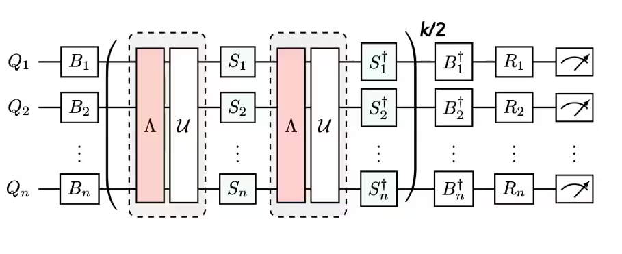
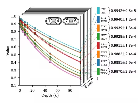
| ส่วนที่ 1 | ส่วนที่ 2 | ส่วนที่ 3 |
|---|---|---|
| Pauli-twirl layer ของ two-qubit gate | ทำซ้ำคู่ layer ที่เป็น identity และเรียนรู้ noise | หา fidelity (error ของแต่ละ noise channel) |
 |  |  |
ภาพรวมการประมวลผลภายหลัง
หลังจากรันบนฮาร์ดแวร์ควอนตัมโดยใช้เฟรมเวิร์ก samplomatic และ Executor เราแปลงผลการวัด bitstring ของเราให้เป็นค่า observable ที่ต้องการ ในบทช่วยสอนนี้ เราสาธิตขั้นตอนการทำงานบนวงจร Ising แบบ mirror (สร้างขึ้นใน Step 1 ด้านล่าง) ซึ่ง expectation value ในอุดมคติของ observable ที่วัดได้คือ 1 เพราะครึ่งหลังของวงจรจะย้อนกลับครึ่งแรก เมื่อคำนวณค่า observable ด้วยฟังก์ชัน executor_expectation_values เราใช้เทคนิคการประมวลผลภายหลังหลายอย่างเพื่อลดผลกระทบของ noise ซึ่งรวมถึงการตัด shot ที่ได้รับผลกระทบจาก noise แบบ non-Markovian, การลด error ของการอ่านค่า (readout-error mitigation) และการคำนึงถึงรายละเอียดของการนำ PEC ของเราไปใช้ รายละเอียดจะถูกกล่าวถึงใน Step 4 ด้านล่าง
ข้อกำหนด
ก่อนเริ่มบทช่วยสอนนี้ ตรวจสอบให้แน่ใจว่าคุณติดตั้งสิ่งต่อไปนี้แล้ว:
-
Qiskit SDK v2.2 ขึ้นไป พร้อมการรองรับ visualization
-
Qiskit Runtime v0.47 ขึ้นไป (
pip install qiskit-ibm-runtime) -
Shaded lightcones Qiskit addon v0.1 ขึ้นไป (
pip install qiskit-addon-slc) -
Qiskit addon utils v0.3 ขึ้นไป (
pip install qiskit-addon-utils) -
Samplomatic v0.13 ขึ้นไป (
pip install samplomatic)
การตั้งค่า
ก่อนอื่น ให้นำเข้าแพ็กเกจและฟังก์ชันที่จำเป็นสำหรับการรัน notebook นี้
# Added by doQumentation — required packages for this notebook
!pip install -q matplotlib numpy qiskit qiskit-addon-slc qiskit-addon-utils qiskit-ibm-runtime samplomatic
from multiprocessing import set_start_method

# Setting this value prevents itertools.starmap deadlock on UNIX systems
set_start_method("spawn")

# Needed to prevent PySCF from parallelizing internally (SLC only)
%set_env OMP_NUM_THREADS=1
env: OMP_NUM_THREADS=1
import numpy as np
from matplotlib import pyplot as plt

from qiskit import QuantumCircuit
from qiskit.quantum_info import SparsePauliOp
from qiskit.transpiler import generate_preset_pass_manager, PassManager

from qiskit_ibm_runtime import (
    QiskitRuntimeService,
    QuantumProgram,
    Executor,
    NoiseLearnerV3,
)

import samplomatic
from samplomatic.utils import find_unique_box_instructions
from samplomatic.transpiler import generate_boxing_pass_manager

from qiskit_addon_utils.exp_vals.measurement_bases import (
    get_measurement_bases,
)
from qiskit_addon_utils.exp_vals.expectation_values import (
    executor_expectation_values,
)
from qiskit_addon_utils.noise_management import (
    gamma_from_noisy_boxes,
    trex_factors,
)
from qiskit_addon_utils.noise_management.post_selection import PostSelector
from qiskit_addon_utils.noise_management.post_selection.transpiler.passes import (
    AddPostSelectionMeasures,
    AddSpectatorMeasures,
)

from qiskit_addon_slc.bounds import (
    compute_backward_bounds,
    compute_forward_bounds,
    compute_local_scales,
    merge_bounds,
    tighten_with_speed_limit,
)
from qiskit_addon_slc.utils import (
    generate_noise_model_paulis,
    map_modifier_ref_to_ref,
)
from qiskit_addon_slc.visualization import draw_shaded_lightcone
ตัวอย่างซิมูเลเตอร์ขนาดเล็ก
เช่นเดียวกับวิธีการลด error แบบอิงการเรียนรู้อื่น ๆ PEC ที่ใช้ shaded lightcone จะลด noise ทางกายภาพ ของ quantum processor ตัวใดตัวหนึ่งโดยเฉพาะ ดังนั้นจึงขึ้นอยู่กับบริการฮาร์ดแวร์ที่ไม่มีความคล้ายคลึงเชิงความหมายบนซิมูเลเตอร์ในอุดมคติ:
-
NoiseLearnerV3กำหนดลักษณะเฉพาะของ sparse Pauli-Lindblad noise channel บน layer แบบ two-qubit ที่ไม่ซ้ำกันแต่ละอันด้วยการทดลอง บนซิมูเลเตอร์ที่ไม่มี noise จะไม่มี noise ให้หักล้าง -
primitive
Executorสุ่มตัวอย่างวงจรที่ถูก twirl และฉีด anti-noise แล้วซึ่งสร้างโดยsamplomaticบน backend
การคำนวณขอบเขตของ shaded-lightcone เป็นการคำนวณเชิงคลาสสิก แต่มีความหมายก็ต่อเมื่อเทียบกับอัตรา noise ของฮาร์ดแวร์ที่เรียนรู้แล้ว ซึ่งกำหนดงบประมาณการลด error และ sampling overhead ด้วยเหตุนี้เราจึงข้ามตัวอย่างซิมูเลเตอร์ขนาดเล็กและสาธิตขั้นตอนการทำงาน PEC+SLC แบบเต็มโดยตรงบนฮาร์ดแวร์ โดยแยกแต่ละขั้นตอนของ Qiskit pattern ไว้ด้านล่าง
ตัวอย่างฮาร์ดแวร์ขนาดใหญ่
เรารันขั้นตอนการทำงาน PEC+SLC แบบสมบูรณ์บนวงจร Ising แบบ mirror ที่มี 20 qubit ซึ่งรันบนฮาร์ดแวร์ IBM Quantum® ตามสี่ขั้นตอนของ Qiskit pattern
ขั้นตอนที่ 1: กำหนดปัญหา
การสาธิตของเราตั้งค่าไว้ดังนี้:
-
เราเลือกที่จะทำ time evolution ภายใต้ Hamiltonian ของ 1D Ising chain 1D Ising chain ให้โครงสร้างวงจรที่หนาแน่นอย่างเหมาะสม ซึ่งสะดวกสำหรับการสาธิตการนำ PEC ไปใช้
-
เราเลือกที่จะวัด observable ซึ่งมีองค์ประกอบ หนึ่งตัวและ หนึ่งตัว สิ่งนี้สะดวกสำหรับการเน้นให้เห็นว่าขอบเขตของ SLC จัดการกับ error ประเภทต่าง ๆ แตกต่างกันอย่างไร
-
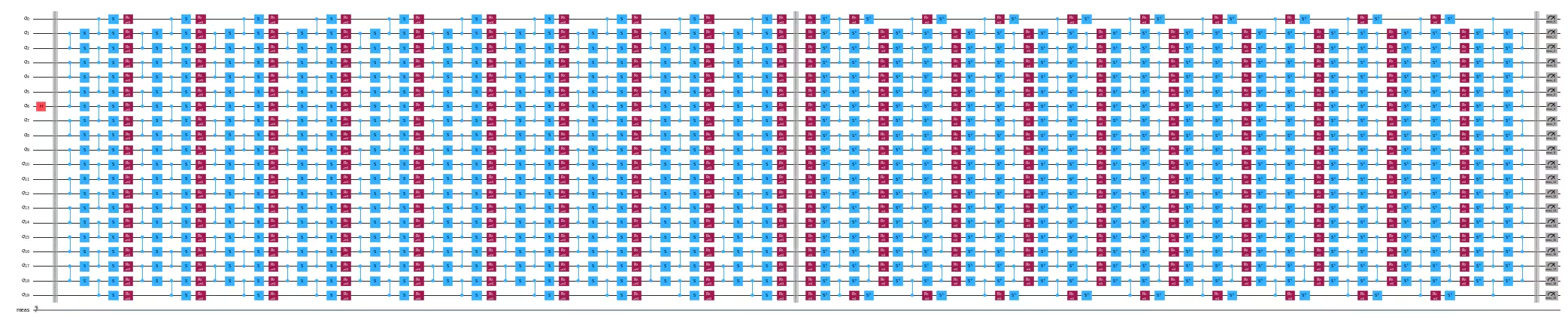
เราต้องการให้ expectation value ในอุดมคติของ observable นี้เท่ากับ 1 พอดี เพื่อให้ตัดสินคุณภาพของค่าประมาณที่ถูกลด error ได้ง่าย การทำ mirror วงจรทำให้เราไปถึงจุดนั้นได้เกือบทั้งหมด: สำหรับทุก gate ในครึ่งหลังของวงจรจะมี gate ผกผันอยู่ในครึ่งแรก ทำให้วงจรในอุดมคติทำหน้าที่เป็น identity
-
สุดท้าย การได้ expectation value ในอุดมคติเท่ากับ 1 ต้องการให้วงจรเริ่มต้น — และด้วยเหตุนี้ เนื่องจากมีการ mirror จึงควรจบลงด้วย — ที่ +1 eigenstate ของ observable เนื่องจาก observable มีองค์ประกอบที่ไม่ใช่ และ primitive
Executorคำนึงถึง measurement basis ที่ต้องการที่ปลายวงจร เราจึงเติม gate เตรียม basis ที่สอดคล้องกันไว้ที่จุดเริ่มต้นของวงจร mirror ด้วยฟังก์ชันprepare_basisเราใช้ฟังก์ชันget_measurement_basesเพื่อระบุว่า gate ใดจำเป็นและควรวางไว้ที่ใด พร้อมทั้งติดตามรายละเอียดปลีกย่อยของดัชนี qubit ที่เกิดจากข้อตกลงของ annotationboxตามที่กล่าวถึงในหัวข้อการเตรียมการวัด canonical basis
# Width of the Ising chain (a free parameter of this demonstration)
num_qubits = 20

# The observable to measure: one X component (on qubit 6) and one Z component
# (on qubit 13), as motivated in "Step 1: Map the problem" above
target_obs_sparse = [("XZ", [6, 13], 1.0)]
observable = SparsePauliOp.from_sparse_list(
    target_obs_sparse, num_qubits=num_qubits
)
# Determine the measurement basis each qubit requires for this observable.
# The reverser is used during post-processing in Step 4.
bases_virt, reverser_virt = get_measurement_bases(observable)
# Free parameters of the demonstration circuit: the number of Trotter steps
# sets the circuit depth, and rx_angle is the transverse-field rotation angle
# applied in each step (pi/4 makes the dynamics non-Clifford)
num_trotter_steps = 10
rx_angle = np.pi / 4
def construct_ising_circuit(
    num_qubits: int,
    num_trotter_steps: int,
    rx_angle: float,
) -> QuantumCircuit:
    circuit = QuantumCircuit(num_qubits)

    for _ in range(num_trotter_steps):
        circuit.rx(rx_angle, range(num_qubits))
        for first_qubit in (1, 2):
            for idx in range(first_qubit, num_qubits, 2):
                # equivalent to Rzz(-pi/2):
                circuit.sdg([idx - 1, idx])
                circuit.cz(idx - 1, idx)

    return circuit

def prepare_basis(
    circuit: QuantumCircuit, basis: list[int]
) -> QuantumCircuit:
    # basis is a list of integer values from 0 to 3. These map to the basis measurement as:
    # 0 = I; 1 = Z; 2 = X; 3 = Y
    assert len(basis) == circuit.num_qubits

    out_circ = circuit.copy_empty_like()
    for qb, bas in enumerate(basis):
        if bas == 2:
            out_circ.h(qb)
        elif bas == 3:
            out_circ.rx(-np.pi / 2, qb)

    out_circ.barrier()
    out_circ.compose(circuit, inplace=True)
    return out_circ

def mirror_circuit(circuit: QuantumCircuit) -> QuantumCircuit:
    mirror_circ = circuit.copy_empty_like()
    mirror_circ.compose(circuit.inverse(), inplace=True)
    mirror_circ.barrier()
    mirror_circ.compose(circuit, inplace=True)
    mirror_circ.measure_active()
    return mirror_circ
# Instantiate the mirrored circuit and prepend the basis-preparation gates
circuit = construct_ising_circuit(num_qubits, num_trotter_steps, rx_angle)
mirrored_circuit = mirror_circuit(circuit)
mirrored_circuit = prepare_basis(mirrored_circuit, bases_virt[0])
mirrored_circuit.draw(
    "mpl", fold=-1, scale=0.3, idle_wires=False, measure_arrows=False
)
ขั้นตอนที่ 2: ปรับให้เหมาะสม
เราปรับรายละเอียดที่เกี่ยวข้องกับวงจรที่จะรัน, observable ที่จะวัด และพารามิเตอร์การเรียนรู้ noise ให้เหมาะสม เริ่มต้น เราเลือกโปรเซสเซอร์ Heron ที่มีคิวว่างมากที่สุด และตั้งค่าให้เปิดใช้งาน fractional gate gate แบบ fractional เหล่านี้ช่วยให้มีความไวมากขึ้นในการกรอง post-selection บางส่วนของเรา
# Initialize IBM Quantum Compute Service using your saved credentials
service = QiskitRuntimeService()

# Select the least busy Heron device. This tutorial targets Heron processors:
# the usage estimate and the non-Markovian-noise post-selection discussed in
# Step 4 are specific to this processor family.
backend = service.least_busy(
    operational=True,
    simulator=False,
    filters=lambda b: b.processor_type["family"] == "Heron",
)
# Re-fetch with fractional gates enabled (least_busy does not forward this)
# Fractional gates are enabled so the non-Clifford Rx rotations are supported natively.
backend = service.backend(backend.name, use_fractional_gates=True)
print(f"Selected backend: {backend.name}")
Selected backend: ibm_kingston
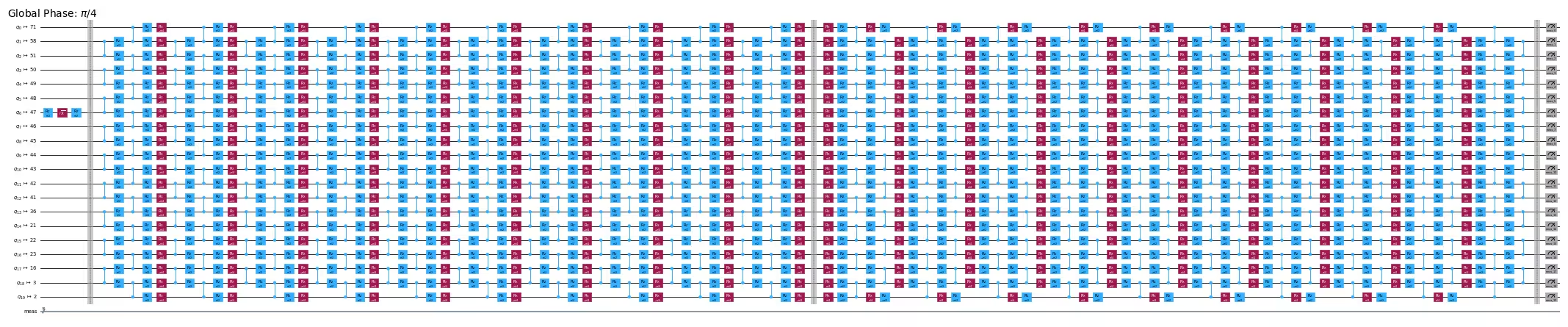
ก่อนอื่น เราจะทำการ transpile วงจรของเราให้เป็นคำสั่ง ISA ตามที่จำเป็นสำหรับการรันบน QPU ของเรา การเลือก qubit ทางกายภาพที่จะรันมีผลกระทบอย่างมากต่อคุณภาพของผลลัพธ์ เนื่องจากเวลา coherence และ fidelity ของ gate แตกต่างกันไปตามอุปกรณ์และเปลี่ยนแปลงไปตามเวลา สำหรับการทดลองที่ต้องการความรอบคอบ การเลือก chain ของ qubit ด้วยมือโดยอิงจากการทดลอง benchmark อย่างรวดเร็วอาจคุ้มค่า (ดูตัวอย่างเช่นบทช่วยสอน Real-time benchmarking for qubit selection) สำหรับวัตถุประสงค์ของบทช่วยสอนนี้ เราอาศัย Qiskit transpiler ในการเลือก layout โดยอิงจาก coupling map ของ backend และข้อมูล calibration ล่าสุด
isa_pm = generate_preset_pass_manager(backend=backend, optimization_level=1)

isa_circuit = isa_pm.run(mirrored_circuit)

# The chain of physical qubits selected by the transpiler
layout = isa_circuit.layout.final_index_layout()
print(f"Selected layout: {layout}")

isa_observable = observable.apply_layout(
    layout, num_qubits=isa_circuit.num_qubits
)
Selected layout: [71, 58, 51, 50, 49, 48, 47, 46, 45, 44, 43, 42, 41, 36, 21, 22, 23, 16, 3, 2]
wire_order = layout + [
    q for q in range(isa_circuit.num_qubits) if q not in layout
]
isa_circuit.draw(
    "mpl",
    fold=-1,
    scale=0.3,
    idle_wires=False,
    wire_order=wire_order,
    measure_arrows=False,
)
จัดวงจรเป็น box
เพื่อความสะดวกในการนำไปใช้ เราใช้ transpilation pass generate_boxing_pass_manager ซึ่งจัดคำสั่งของวงจรลงใน box ที่มี annotation box เหล่านี้ระบุอย่างชัดเจนว่า ในกรณีของ PEC ควรฉีด anti-noise ที่ใดในวงจร สำหรับรายละเอียดของการตั้งค่า โปรดดู เอกสาร Samplomatic
โปรดทราบว่าขั้นตอนการทำงาน SLC จำเป็นต้องใช้ inject_noise_strategy="individual_modification" ในขั้นตอนถัดไป เนื่องจากสิ่งนี้ช่วยให้เราสามารถระบุ annotation InjectNoise ของคำสั่ง BoxOp ในวงจรได้อย่างเฉพาะเจาะจง (box ที่ไม่มี annotation InjectNoise ไม่สามารถระบุได้ด้วยวิธีนี้)
การคำนวณ SLC bound ในปัจจุบันสมมติว่า annotation InjectNoise ถูกวางด้วย site="after" (ดู qiskit-addon-slc#33) เนื่องจากค่าเริ่มต้นของการตั้งค่านี้เปลี่ยนแปลงใน samplomatic เวอร์ชันล่าสุด (ดู samplomatic#372) เราจึงตั้งค่า inject_noise_site="after" อย่างชัดเจนด้านล่าง
ฟังก์ชัน find_unique_box_instructions จะวนซ้ำผ่านวงจรที่ถูกจัดเป็น box ที่ให้มา และระบุ box ที่มี layer แบบ two-qubit (2Q) หรือการวัดที่ไม่ซ้ำกัน เพื่อวัตถุประสงค์ในการเรียนรู้และฉีด noise
# Box circuit with Twirl and InjectNoise annotations
boxes_pm = generate_boxing_pass_manager(
    twirling_strategy="active",
    inject_noise_strategy="individual_modification",
    inject_noise_site="after",
    inject_noise_targets="gates",
    measure_annotations="all",
)

boxed_circuit = boxes_pm.run(isa_circuit)

# Find the unique instructions (layers) from boxed circuit
unique_2q_instructions = find_unique_box_instructions(
    boxed_circuit, normalize_annotations=None, undress_boxes=True
)
boxed_circuit.draw(
    "mpl",
    fold=-1,
    scale=0.3,
    idle_wires=False,
    wire_order=wire_order,
    measure_arrows=False,
)

เตรียมการวัด canonical basis
โปรดทราบว่าเราต้องระมัดระวังเป็นพิเศษในการติดตามลำดับ qubit ด้านล่างนี้ เราแนะนำแนวคิดของ canonical_qubits เป็นวิธีในการอัปเดตลำดับ qubit ให้เหมาะสมเมื่อส่งไปยัง Executor อันเป็นผลมาจากวิธีที่ลำดับ qubit ถูกบันทึกไว้เมื่อจัดวงจรเป็น box และค้นหาคำสั่งที่ไม่ซ้ำกัน ดูเอกสาร Qubit ordering convention สำหรับรายละเอียด
# Determine the canonical qubits order
meas_box = boxed_circuit.data[-1]
canonical_qubits = [
    idx
    for idx, qubit in enumerate(boxed_circuit.qubits)
    if qubit in meas_box.qubits
]

# map canonical qubit to physical (isa) qubit
c_2_p = {c: p for c, p in enumerate(canonical_qubits)}
# map physical (isa) qubit to virtual qubit (index in original circuit)
p_2_v = {p: v for v, p in enumerate(layout)}
# compute map between virtual and canonical qubit indices.
c_2_v = {c: p_2_v[p] for c, p in c_2_p.items()}

assert len(c_2_v) == num_qubits

bases_canon = [
    np.array([base_i[c_2_v[c]] for c in range(num_qubits)], dtype=np.uint8)
    for base_i in bases_virt
]
ขั้นตอนการทำงานสำหรับการเฉด lightcone, การเรียนรู้ noise และการฉีด anti-noise
ในบทช่วยสอนนี้ เราจะรันการคำนวณ SLC bound ก่อนที่ noise learning จะเสร็จสมบูรณ์ เพื่อให้ circuit ที่จะถูก mitigate ถูกรันในเวลาที่ใกล้เคียงกับ noise model ที่เรียนรู้มากที่สุด โดยหลักการแล้ว workflow นี้สามารถขนานกันได้มากขึ้นไปอีก: noise-learning job สามารถรันไปพร้อม ๆ กับการประมาณค่า noise bound ได้ สำหรับ quantum circuit ใด ๆ การคำนวณ noise-bound สามารถขยายขนาดด้วย dependency แบบ exponential ที่อ่อน ดังนั้นการทำการคำนวณ bound แบบขนาน (ตัวอย่างเช่น บน CPU core หลาย ๆ ตัว) จะให้ bound ที่แน่นขึ้นสำหรับงบประมาณเวลาการคำนวณที่กำหนด และการรัน QPU กับการคำนวณ bound เองก็สามารถทำแบบขนานกันได้เพื่อ workflow ที่มีประสิทธิภาพสูงสุด
ทำนาย Pauli ของ noise model ที่จะเรียนรู้
ก่อนที่จะรันการเรียนรู้ noise ใด ๆ บนฮาร์ดแวร์ เราจะแจกแจง Pauli error term ที่ noise model ของเราจะมีก่อน จำไว้ว่าเราจำลอง noise ของแต่ละ layer ที่ไม่ซ้ำกันเป็น sparse Pauli-Lindblad model ที่มีอัตรา error หนึ่งอัตราสำหรับ weight-one Pauli แต่ละตัว (, หรือ ) บน qubit ที่ active แต่ละตัว และหนึ่งอัตราสำหรับ weight-two Pauli แต่ละตัวบนคู่ qubit ที่ active ที่เชื่อมต่อกันแต่ละคู่ ฟังก์ชัน generate_noise_model_paulis จะวนซ้ำผ่าน layer ที่จัดเป็น box ที่ไม่ซ้ำกันแต่ละอันของวงจรที่ให้มา และสร้างรายการ Pauli term นี้ขึ้นมาอย่างแม่นยำ โดยคำนึงถึงการเชื่อมต่อของ qubit ในวงจร
กล่าวอีกนัยหนึ่ง ขั้นตอนนี้ทำนาย โครงสร้าง ของ noise model ที่ NoiseLearnerV3 จะเติมเต็มด้วยอัตราที่เรียนรู้แล้วในภายหลัง การรู้โครงสร้างนี้ล่วงหน้าคือสิ่งที่ทำให้เราสามารถคำนวณขอบเขตแบบ forward และ backward สำหรับ error ที่เป็นไปได้ทุกตัวได้ ก่อนที่การเรียนรู้ noise จะรันเสียด้วยซ้ำ
noise_model_paulis = generate_noise_model_paulis(
    unique_2q_instructions, backend.coupling_map, boxed_circuit
)
noise_model_rates = {ref: None for ref in noise_model_paulis}
a. คำนวณขอบเขตแบบ forward
ฟังก์ชัน compute_forward_bounds ประเมินความสัมพันธ์การสลับที่ (commutation relations) ระหว่าง gate ในแต่ละ layer และ Pauli term ที่สร้างขึ้นข้างต้น ในแง่ของวิธีที่ error แบบ forward-propagation ส่งผลต่อ observable ที่ต้องการ สำหรับ gate ที่สลับที่ได้กับ Pauli term จะไม่มีการดำเนินการใด ๆ สำหรับ Clifford gate จะถูกผลักไปทางจุดเริ่มต้นของวงจร สำหรับ non-Clifford gate เราประมาณอิทธิพลของมันต่อ observable เป้าหมายเพื่อนำไปจัดลำดับความสำคัญสำหรับการหักล้าง noise ในภายหลัง (หลังจากขอบเขตทั้งหมดถูกรวมเข้าด้วยกันแล้ว) ขอบเขตนี้ได้มาโดยการใช้ L2 norm ก่อน (นั่นคือ รากที่สองของผลรวมกำลังสองของสัมประสิทธิ์ Pauli term ที่เกี่ยวข้อง) เมื่อมี qubit term ที่เกี่ยวข้องมากเกินไป เราจะย้อนกลับไปใช้ขอบเขตที่หลวมกว่าซึ่งใช้ triangle inequality
ตั้งค่าพารามิเตอร์การคำนวณขอบเขต
การตั้งค่าต่อไปนี้ควบคุมการคำนวณขอบเขตเชิงคลาสสิก:
-
slc_atol: ค่าความคลาดเคลื่อนสัมบูรณ์ของการคำนวณ operator term ที่มีสัมประสิทธิ์ต่ำกว่าเกณฑ์นี้จะถือว่าไม่สำคัญและถูกทิ้งไป -
slc_eigval_max_qubits: จำนวน qubit สูงสุดที่ขอบเขตแบบ eigenvalue-based (L2-norm) ที่แน่นกว่าจะถูกประเมิน operator ที่มี support ครอบคลุม qubit มากกว่านี้จะถอยไปใช้ขอบเขตแบบ triangle-inequality ที่หลวมกว่าซึ่งอธิบายไว้ข้างต้น -
slc_evolution_max_terms: จำนวน Pauli term สูงสุดที่คงไว้ระหว่างการแพร่กระจาย operator ผ่านวงจร การตัด term ที่เล็กที่สุดออกช่วยให้การคำนวณสามารถจัดการได้ โดยแลกกับขอบเขตที่หลวมขึ้นเล็กน้อย -
slc_num_processes: จำนวน CPU process ที่การคำนวณขอบเขตถูกกระจายทำงานแบบขนาน -
slc_timeout: งบประมาณเวลา (เป็นวินาที) สำหรับการคำนวณขอบเขต layer ใด ๆ ที่ไม่ถูกเข้าถึงภายในงบประมาณนี้จะถูกกำหนดขอบเขตแบบ trivial เป็น 2
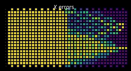
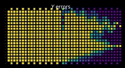
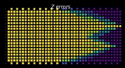
ในบทช่วยสอนนี้ เราจงใจให้เกิด timeout: เรากำหนดให้ slc_timeout มีค่าน้อยโดยเจตนา เพื่อให้ notebook รันได้อย่างรวดเร็ว และเพื่อแสดงให้เห็นว่าการไปถึง timeout นั้นปลอดภัย ค่า shade ที่คำนวณได้เป็น upper bound ในทุกขั้นตอน ดังนั้นการไปถึง timeout จะทำให้ bound หลวมขึ้น (trivial) เฉพาะสำหรับ layer ที่ยังไปไม่ถึงเท่านั้น มันไม่เคยประเมินผลกระทบของ error ต่ำเกินไป สิ่งนี้ปรากฏในภาพแสดงผลด้านล่างเป็น layer ทางซ้ายสุดที่ถูกเติมเต็มด้วย trivial bound ทั้งหมด การเพิ่ม timeout (หรือจำนวน process) จะทำให้ bound แน่นขึ้นและลด sampling overhead ลงไปอีก
slc_atol = 1e-8
slc_eigval_max_qubits = 18
slc_evolution_max_terms = 1000
slc_num_processes = 8
slc_timeout = 60
forward_bounds = compute_forward_bounds(
    boxed_circuit,
    noise_model_paulis,
    isa_observable,
    evolution_max_terms=slc_evolution_max_terms,
    eigval_max_qubits=slc_eigval_max_qubits,
    atol=slc_atol,
    num_processes=slc_num_processes,
    timeout=slc_timeout,
)
Bounds computation timed out.
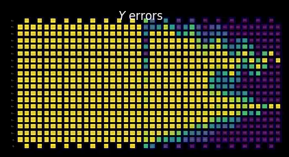
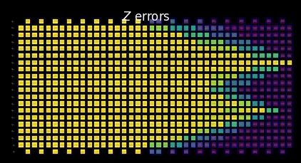
แสดงภาพ SLC เพื่อตรวจสอบด้วยตนเอง
คุณสามารถตีความพฤติกรรมของขอบเขตที่เฉดโดยตรวจสอบว่าการวัดและ Pauli term มีปฏิสัมพันธ์กับ error ท้องถิ่นอย่างไร รูปแบบเหล่านี้เป็นลักษณะเฉพาะของปัญหา time-evolution ของ kicked Ising Hamiltonian นี้ และยังปรากฏในบทความ Lightcone Shading for Classically Accelerated Quantum Error Mitigation พร้อมด้วยคุณลักษณะบ่งชี้หลายประการ:
-
เราสามารถแยกแยะกรวยทั้งสองที่เกิดจาก non-identity Pauli ทั้งสองใน observable ได้อย่างชัดเจน
-
เราสามารถเห็นได้ว่าการวัด X บน qubit 6 สลับที่ได้กับ X error ใน layer ที่อยู่ขวาสุด
-
เราสามารถเห็นได้ว่า Z Pauli บน qubit 13 สลับที่ได้กับ Z error ใน layer ที่อยู่ขวาสุด
-
เมื่อเราถึงเวลา timeout ที่ระบุไว้ข้างต้น layer ที่เหลือทางด้านซ้ายจะถูกเติมเต็มทั้งหมดด้วยขอบเขตแบบ trivial ที่ค่าสอง
for p in "XYZ":
    display(
        draw_shaded_lightcone(
            boxed_circuit,
            forward_bounds,
            noise_model_paulis,
            pauli_filter=p,
            scale=0.15,
            fold=-1,
            idle_wires=False,
            wire_order=wire_order,
            measure_arrows=False,
        )
    )
b. จำกัดขอบเขตแบบ forward ให้แน่นขึ้นด้วย quantum speed limit
ต่อไปเราจะจำกัดขอบเขตให้แน่นขึ้นโดยใช้ฟังก์ชัน tighten_with_speed_limit การแพร่กระจายเชิงเรขาคณิตของ lightcone ของ observable ถูกคำนึงถึงอย่างครบถ้วนแล้วในขอบเขตแบบ forward ที่คำนวณข้างต้น สิ่งที่ฟังก์ชันนี้เพิ่มเข้ามาคือการทำ self-consistency pass ที่ใช้ประโยชน์จากความเร็วจำกัดที่ข้อมูลสามารถไหลผ่านวงจรได้ — lightcone ขยายได้มากที่สุดหนึ่ง qubit ต่อ layer ของ two-qubit gate — เพื่อจำกัดขอบเขตที่คำนวณไว้ก่อนหน้านี้ให้แน่นขึ้นเมื่อเทียบกัน ข้อมูลไหลไปทั้งสองทิศทาง:
-
จากขอบเขต commutator ไปยังขอบเขตของ observable ที่ backpropagated แล้ว: ถ้า observable สลับที่ได้กับ error บน qubit หนึ่ง มันก็ไม่สามารถมีองค์ประกอบ หรือ มากนักที่นั่น
-
จากขอบเขตของ observable ที่ backpropagated แล้วไปยังขอบเขต commutator: ถ้า observable มีองค์ประกอบ และ เพียงเล็กน้อยบน qubit หนึ่ง มันก็เกือบจะสลับที่ได้กับ ที่นั่น
forward_bounds_tighter = tighten_with_speed_limit(
    forward_bounds, boxed_circuit, noise_model_paulis, isa_observable
)
แสดงภาพ SLC เพื่อตรวจสอบด้วยตนเอง
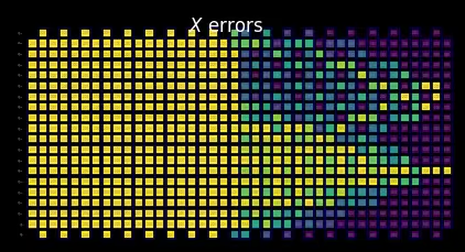
โดยหลักการแล้ว การทำให้แน่นขึ้นนี้ให้การเปลี่ยนผ่านที่ราบรื่นกว่าระหว่างขอบเขตที่คำนวณได้และขอบเขตแบบ trivial ที่กำหนดให้กับ layer ที่เกิน timeout ในตัวอย่างนี้ ผลกระทบแทบมองไม่เห็น เพราะ lightcone ได้แพร่กระจายไปถึงขอบของวงจรแล้วเมื่อถึงเวลา timeout
for p in "XYZ":
    display(
        draw_shaded_lightcone(
            boxed_circuit,
            forward_bounds_tighter,
            noise_model_paulis,
            pauli_filter=p,
            scale=0.15,
            fold=-1,
            idle_wires=False,
            wire_order=wire_order,
            measure_arrows=False,
        )
    )
c. คำนวณขอบเขตแบบ backward
ส่วนนี้ของการทำนาย noise ประเมินว่า error ที่ layer ใดหนึ่งสามารถส่งผลต่อ input state อย่างไร ฟังก์ชัน compute_backward_bounds จะกลับวงจรก่อน และลบ gate การวัดออก แล้วดำเนินการวิเคราะห์ที่คล้ายกับที่ทำสำหรับการคำนวณขอบเขตแบบ forward
backward_bounds = compute_backward_bounds(
    boxed_circuit,
    noise_model_paulis,
    evolution_max_terms=slc_evolution_max_terms,
    num_processes=slc_num_processes,
    timeout=slc_timeout,
)
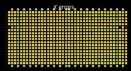
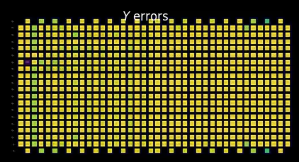
แสดงภาพ SLC เพื่อตรวจสอบด้วยตนเอง
จากการคำนวณขอบเขตแบบ backward เราสามารถเห็นได้ว่าโครงสร้างของ initial state ควบคุมพฤติกรรมช่วงต้นของการแพร่กระจาย error อย่างไร:
-
เราสามารถเห็นได้อย่างชัดเจนว่า Z error สลับที่ได้กับ initial state |0⟩ ในช่วงแรก
-
เฉพาะบน qubit 6 ซึ่งเราตั้งค่าเริ่มต้นเป็น +1 eigenstate ของ X basis เท่านั้น ที่ Z error ไม่สลับที่ ในขณะที่ X error สลับที่ได้
for p in "XYZ":
    display(
        draw_shaded_lightcone(
            boxed_circuit,
            backward_bounds,
            noise_model_paulis,
            pauli_filter=p,
            scale=0.15,
            fold=-1,
            idle_wires=False,
            wire_order=wire_order,
            measure_arrows=False,
        )
    )
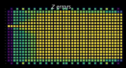
แสดงตัวอย่างขอบเขตที่รวมกันโดยไม่มีอัตรา noise ที่เรียนรู้แล้ว
ฟังก์ชัน merged_bounds กำหนดจุดในวงจรที่การเปลี่ยนจากขอบเขตแบบ backward ไปเป็นแบบ forward ทำให้ bias โดยประมาณทั้งหมดของ observable ที่ต้องการมีค่าต่ำที่สุด bias นี้คำนวณเป็นผลรวมของส่วนสนับสนุนขอบเขตแบบ backward สำหรับตำแหน่ง noise ทั้งหมดก่อนจุดนั้น บวกกับส่วนสนับสนุนขอบเขตแบบ forward สำหรับตำแหน่ง noise ทั้งหมดหลังจากนั้น ปัจจุบัน สิ่งนี้ทำอย่างสม่ำเสมอสำหรับ qubit ทั้งหมด
จุดที่เหมาะสมในการเปลี่ยนจากขอบเขตแบบ backward ไปเป็น forward ขึ้นอยู่กับอัตรา noise ที่เรียนรู้แล้ว ในขั้นตอนนี้เรายังไม่ได้เรียนรู้อัตราใด ๆ: noise_model_rates ถูกกำหนดค่าเริ่มต้นเป็น None สำหรับทุก layer ซึ่ง merge_bounds จะถือว่าเป็นอัตรา noise ที่สม่ำเสมอ ขอบเขตที่รวมกันที่แสดงที่นี่จึงเป็นเพียงตัวอย่างเท่านั้น เราจะคำนวณใหม่ด้วยอัตราที่เรียนรู้จริงใน Step 3
merged_bounds = merge_bounds(
    boxed_circuit,
    forward_bounds_tighter,
    backward_bounds,
    noise_model_rates,
)
Missing noise rates. Partitioning backward/forward commutator bounds by assuming uniform error rates.
Optimal spacetime partitioning not implemented!Just partitioning list of noisy boxes.
แสดงภาพ SLC เพื่อตรวจสอบด้วยตนเอง
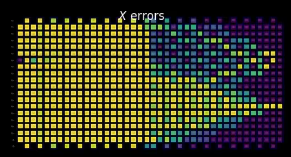
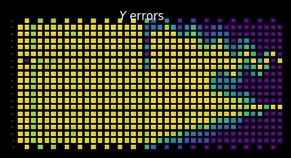
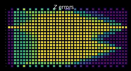
หลังจากรวมขอบเขตแบบ backward และแบบ forward ที่ปรับให้แน่นขึ้นแล้ว พฤติกรรมของ SLC ที่รวมกันจะชัดเจนขึ้น:
-
ฟังก์ชันข้างต้นบอกเราว่ามีการเลือกจุดแบ่งที่การเปลี่ยนจากขอบเขตแบบ backward ไปเป็นแบบ forward ที่ปรับให้แน่นขึ้นเกิดขึ้น
-
เราสามารถเห็นด้านล่างว่า SLC ในตอนนี้มีขอบเขตแบบ backward บางส่วนและขอบเขตแบบ forward ที่ปรับให้แน่นขึ้นบางส่วน
for p in "XYZ":
    display(
        draw_shaded_lightcone(
            boxed_circuit,
            merged_bounds,
            noise_model_paulis,
            pauli_filter=p,
            scale=0.15,
            fold=-1,
            idle_wires=False,
            wire_order=wire_order,
            measure_arrows=False,
        )
    )
ขั้นตอนที่ 3: รัน
ในส่วนนี้ เราเริ่มส่วนของขั้นตอนการทำงานที่ใช้อุปกรณ์ควอนตัมจริง สำหรับวิธีการลด error แบบอิงการเรียนรู้นี้ มีสองขั้นตอน:
-
เรียนรู้ noise โดยใช้
NoiseLearnerV3 -
รันวงจรการลด error ด้วยเฟรมเวิร์ก
samplomaticและExecutor
ด้วยขอบเขต error ที่ถูกจำกัดจากวงจรควอนตัมของเรา เราเรียนรู้อัตรา noise ที่เกี่ยวข้องเพื่อจัดลำดับความสำคัญของงบประมาณ error ของเรา กำหนด sampling overhead และรันบน QPU
a. เรียนรู้อัตรา noise
noise learner กำหนดลักษณะเฉพาะของกระบวนการ noise ที่ส่งผลต่อ gate ในวงจรที่สนใจหนึ่งวงจรหรือมากกว่า โดยอิงจาก Pauli-Lindblad noise model แบบ sparse เมธอด run() เริ่มงานการเรียนรู้ noise สำหรับ layer แบบ two-qubit ที่ไม่ซ้ำกันที่ให้มา โดยใช้ตัวเลือกที่ระบุไว้ในการกำหนดค่า noise learner ตัวเลือกเหล่านี้ควบคุมกลยุทธ์ Pauli-twirling, จำนวนการสุ่ม (randomization) และ shot, ความลึกในการเรียนรู้ และ post-selection
เรายังเลือกความลึกในการเรียนรู้อย่างจงใจด้วย ข้อค้นพบเชิงปฏิบัติสำหรับการลด error แบบอิงการเรียนรู้ด้วย samplomatic คือ การให้ความลึกในการเรียนรู้ที่ลึกที่สุดตรงกับความลึกของวงจรที่คุณต้องการลด error นั้นมีประโยชน์อย่างมาก เนื่องจาก layer_pair_depths ของ NLv3 วัดเป็น layer pair (layer หนึ่งบวกกับตัวผกผันของมัน) เราจึงตั้งค่าที่ลึกที่สุดเป็นครึ่งหนึ่งของความลึก two-qubit-layer ของวงจร
post_selection_enabled = True
# Match the deepest noise-learning depth to the depth of the circuit being
# mitigated. NLv3 ``layer_pair_depths`` are measured in layer pairs (a layer
# plus its inverse), so the deepest value is half the circuit's two-qubit-layer
# depth. Learning to this depth markedly improves the quality of the mitigation.
#
# We measure the two-qubit-layer depth on the pre-boxed ISA circuit: after
# boxing, every two-qubit gate is hidden inside a full-width ``BoxOp``, so a
# ``num_qubits == 2`` filter on ``boxed_circuit`` matches nothing (and
# ``QuantumCircuit.depth`` does not recurse into boxes).
depth_2q = isa_circuit.depth(lambda instr: instr.operation.num_qubits == 2)
max_layer_pair_depth = depth_2q // 2  # dividing by 2 since we want pairs

# Use a fixed schedule of learning depths, but drop any that exceed the circuit's
# depth and always cap the deepest value at ``max_layer_pair_depth`` so we never
# learn deeper than the circuit being mitigated.
candidate_depths = [1, 2, 4, 8, 12, 16, 24, 32, 40, 48]
layer_pair_depths = sorted(
    {d for d in candidate_depths if d < max_layer_pair_depth}
    | {max_layer_pair_depth}
)

noise_learner_options = {
    "num_randomizations": 64,
    "shots_per_randomization": 128,
    "layer_pair_depths": layer_pair_depths,
    "post_selection": {
        "enable": post_selection_enabled,
        "strategy": "edge",
        "x_pulse_type": "rx",
    },
    "environment": {"job_tags": ["TUT_SLC"]},
}

noise_learner = NoiseLearnerV3(backend, noise_learner_options)
noise_learner_job = noise_learner.run(unique_2q_instructions)
noise_learner_result = noise_learner_job.result()
if post_selection_enabled:
    print(
        "Minimum fraction of shots kept for noise learning experiments: ",
        end="",
    )
    print(
        f"{min([min(d.values()) for d in [nlr.metadata['post_selection']['fraction_kept'] for nlr in noise_learner_result[:2]]]):.2f}"
    )
Minimum fraction of shots kept for noise learning experiments: 0.71
# Get a dict mapping each InjectNoise.ref to its learned PauliLindbladMap
refs_2_plm = noise_learner_result.to_dict(
    unique_2q_instructions, require_refs=False
)
b.i. อัปเดตขอบเขตที่รวมกันด้วยอัตรา noise ที่เรียนรู้จริง
เมื่อ noise model เฉพาะเจาะจงถูกเรียนรู้แล้ว เราสามารถนำอัตรา noise ที่เรียนรู้แล้วไปใช้กับขอบเขต noise ที่ทำนายไว้ และได้ข้อสรุปสุดท้ายว่าขอบเขตใดมีผลกระทบมากที่สุดในการลด bias ให้น้อยที่สุด
merged_bounds = merge_bounds(
    boxed_circuit,
    forward_bounds_tighter,
    backward_bounds,
    refs_2_plm,
)
Optimal spacetime partitioning not implemented!Just partitioning list of noisy boxes.
b.ii. คำนวณ local_scales สำหรับการรันบนฮาร์ดแวร์
compute_local_scales จะพิจารณา noise error ที่เป็นไปได้แต่ละตัวในวงจร และประมาณว่า error นั้นจะทำให้เกิด bias ในการวัดครั้งสุดท้ายมากเพียงใด รวมถึงค่าใช้จ่ายในการแก้ไขมันมากเพียงใด จากนั้นจะจัดอันดับ error ตามความคุ้มค่าในการลด และเลือกชุดย่อยที่ลด bias ได้มากที่สุด ในขณะที่ยังคงอยู่ในงบประมาณ sampling-cost ที่อนุญาต (หรือบรรลุความแม่นยำที่ต้องการ) ผลลัพธ์คือชุดของตัวประกอบการปรับสเกลที่ระบุว่า error ใดจะถูกลดอย่างจริงจังและ error ใดจะถูกปล่อยไว้โดยไม่ลด (local_scales) พร้อมด้วย sampling cost overhead รวมที่คาดการณ์ไว้ (sampling_costs) และ bias ที่เหลืออยู่ (residual_bias_bound)
ความสามารถในการควบคุม bias ที่เหลืออยู่ตามที่ต้องการเป็นคุณสมบัติสำคัญของการนำ PEC แบบ SLC มาใช้ ในขณะที่ใน การนำไปใช้ดั้งเดิม sampling overhead มักมุ่งเป้าไปที่ zero bias เสมอ เราสามารถปรับ sampling overhead ที่ต้องการโดยแลกกับ bias ที่เหลืออยู่ที่คาดการณ์ไว้ได้ สิ่งนี้ช่วยให้ผู้ใช้อยู่ในงบประมาณ sampling ที่กำหนดไว้ ซึ่งมีประโยชน์อย่างยิ่งเมื่อเริ่มสร้างต้นแบบขั้นตอนการทำงาน
id_map = map_modifier_ref_to_ref(boxed_circuit)
summed_rates = 0.0
for box_id, noise_id in id_map.items():
    learned_plm = refs_2_plm[noise_id]
    summed_rates += np.sum(learned_plm.rates)
    # print(f"{box_id}:\tgamma = {np.exp(2 * summed_rates):1.6e}\tsampling cost = {np.exp(4 * summed_rates):1.6e}")
total_gamma = np.exp(2 * summed_rates)
print(
    f"Full PEC gamma={total_gamma}, sampling cost (gamma^2) = {total_gamma**2}"
)
Full PEC gamma=12.750876317157042, sampling cost (gamma^2) = 162.58484685543633
biases = []
costs = []
for bias in [0.0] + np.arange(0.001, 0.102, 0.01).tolist():
    _, cost_, bias_ = compute_local_scales(
        boxed_circuit,
        merged_bounds,
        refs_2_plm,
        sampling_cost_budget=np.inf,
        bias_tolerance=bias,
    )
    biases.append(bias_)
    costs.append(cost_)
แลก sampling overhead กับ residual bias
xticks = np.arange(0, 11)

fig, ax = plt.subplots()
ax.scatter(
    [0], [total_gamma**2], marker="D", c="tab:orange", label="full PEC"
)
ax.plot(
    100 * np.array(biases),
    np.array(costs),
    "o-",
    c="tab:blue",
    label="PEC+SLC",
)
ax.set_yscale("log")
ax.set_xticks(xticks, [f"{x:.1f}" for x in xticks])

ax.set_xlabel("Remaining bias [%]")
ax.set_ylabel(r"Sampling overhead, $\gamma^2$")
ax.grid()
ax.legend()
fig.suptitle("PEC sampling overhead reduction due to SLC")
Text(0.5, 0.98, 'PEC sampling overhead reduction due to SLC')

chosen_bias_thres = 0.1
local_scales, sampling_cost, residual_bias_bound = compute_local_scales(
    boxed_circuit,
    merged_bounds,
    refs_2_plm,
    sampling_cost_budget=np.inf,
    bias_tolerance=chosen_bias_thres,
)
print(
    f"PEC+SLC sampling cost (gamma^2) = {sampling_cost} "
    f"w/ remaining bias = {100 * residual_bias_bound:.1f}%"
)
PEC+SLC sampling cost (gamma^2) = 48.13646509622307 w/ remaining bias = 10.0%
c. รันวงจรที่สนใจด้วย antinoise
c.i. เตรียม template circuit โดยใช้ samplex
samplex เป็นผลลัพธ์ของเมธอด build ของ Samplomatic ซึ่งเข้ารหัสข้อมูลทั้งหมดที่จำเป็นสำหรับการสร้างพารามิเตอร์แบบสุ่มสำหรับ template_circuit จากนั้นสิ่งเหล่านี้จะถูกนำไปใช้ตั้งค่าอ็อบเจกต์ QuantumProgram ซึ่งจะถูกรันบน QPU ด้วย primitive Executor แต่ละ QuantumProgram สามารถมีหลายรายการ ซึ่งคุณสามารถมองว่าเป็นคู่ของ template และ samplex
ดูรายละเอียดได้ที่ tutorial Hello samplomatic
# Build template circuit and samplex for later use with the "Executor"
template_circuit, samplex = samplomatic.build(boxed_circuit)
# Set up postselection if it's been enabled
if post_selection_enabled:
    # Set up post selection PM (to add PS instructions)
    post_selection_pm = PassManager(
        [
            AddSpectatorMeasures(backend.coupling_map),
            AddPostSelectionMeasures(x_pulse_type="rx"),
        ]
    )
    final_template_circuit = post_selection_pm.run(template_circuit)
else:
    final_template_circuit = template_circuit
c.ii. ตั้งค่า QuantumProgram
num_randomizations = 4096
shots_per_randomization = 64
chunk_size = 256
# Set up QuantumProgram
program = QuantumProgram(shots=shots_per_randomization, noise_maps=refs_2_plm)

# no EM

# Collect up a dict of the other arguments that need to be bound to samplex_inputs
samplex_inputs = {
    f"noise_scales.{ref}": float(0) for ref in local_scales.keys()
}
samplex_inputs |= {"basis_changes": {"basis0": bases_canon[0]}}

# Convert samplex_inputs into a dict to pass to QuantumProgram
samplex_arguments = (
    samplex.inputs().bind(**samplex_inputs).make_broadcastable()
)

program.append_samplex_item(
    circuit=final_template_circuit,
    samplex=samplex,
    samplex_arguments=samplex_arguments,
    shape=(num_randomizations,),
    chunk_size=chunk_size,
)

# plain PEC

# Collect a dict of the other arguments that need to be bound to samplex_inputs
samplex_inputs = {
    f"noise_scales.{ref}": float(-1) for ref in local_scales.keys()
}
samplex_inputs |= {"basis_changes": {"basis0": bases_canon[0]}}

# Convert samplex_inputs into a dict to pass to QuantumProgram
samplex_arguments = (
    samplex.inputs().bind(**samplex_inputs).make_broadcastable()
)

program.append_samplex_item(
    circuit=final_template_circuit,
    samplex=samplex,
    samplex_arguments=samplex_arguments,
    shape=(num_randomizations,),
    chunk_size=chunk_size,
)

# PEC+SLC

# Collect a dict of the other arguments that need to be bound to samplex_inputs
samplex_inputs = {
    f"noise_scales.{ref}": float(-1) for ref in local_scales.keys()
}
samplex_inputs |= {"basis_changes": {"basis0": bases_canon[0]}}
samplex_inputs |= {"local_scales": local_scales}

# Convert samplex_inputs into a dict to pass to QuantumProgram
samplex_arguments = (
    samplex.inputs().bind(**samplex_inputs).make_broadcastable()
)

program.append_samplex_item(
    circuit=final_template_circuit,
    samplex=samplex,
    samplex_arguments=samplex_arguments,
    shape=(num_randomizations,),
    chunk_size=chunk_size,
)
c.iii. รันโปรแกรมด้วย primitive Executor
executor = Executor(backend)
job_exec = executor.run(program)
results_exec = job_exec.result()
ขั้นตอนที่ 4: ประมวลผลภายหลัง
เนื่องจากเราคำนวณ expectation value สุดท้ายที่สนใจโดยใช้ executor_expectation_values เราจึงนำเทคนิคการประมวลผลภายหลังหลายอย่างมาใช้เพื่อช่วยให้มั่นใจว่าเราจะได้ผลลัพธ์ที่มีคุณภาพสูงที่สุดเท่าที่จะเป็นไปได้ ขั้นแรก เราใช้ twirled readout error extinction (TREX) ของเรา ซึ่งจะจัดการกับ error ใดๆ ที่เกิดขึ้นระหว่างกระบวนการ readout จากนั้น เราแก้ไข error ที่เกิดจาก non-Markovian noise บน Heron backend ของเราโดยใช้วิธีการ post-selection วิธีนี้จะวัด active qubit และ spectator qubit จากนั้นใช้การหมุนแบบช้าๆ กับแต่ละ qubit แล้ววัดอีกครั้ง ในกรณีที่การวัดสองครั้งไม่ยืนยันว่า qubit พลิกกลับตามที่คาดไว้ shot เหล่านี้จะถูกทิ้งโดยใช้ mask จาก PostSelector ภายในการคำนวณ mask สามารถกำหนดกลยุทธ์เฉพาะเพื่อกรองตาม single-qubit node หรือ neighboring spectator edge ซึ่งสามารถส่งผลต่อทั้งจำนวน shot ที่ถูกกรองออกและคุณภาพของผลลัพธ์
measurement_noise_map = noise_learner_result[2].to_pauli_lindblad_map()
trex_scale_factors = trex_factors(measurement_noise_map, reverser_virt)
post_selection_strategy = "node"
def post_process_conv(datum, steps=16, gamma=None, ps=False, trex=False):
    meas = datum["meas"]
    flips = datum["measurement_flips.meas"]
    signs = datum.get("pauli_signs", None)

    meas_basis_axis = None
    avg_axis = 0

    mask = None
    if ps and post_selection_enabled:
        # Post-select the results
        post_selector = PostSelector.from_circuit(
            circuit=final_template_circuit, coupling_map=backend.coupling_map
        )

        # Compute the ps mask for filtering results
        mask = post_selector.compute_mask(
            datum, strategy=post_selection_strategy
        )

        # Compute fraction of shots kept from post selection
        total_num_shots = num_randomizations * shots_per_randomization
        ps_ratio = np.sum(mask) * 100 / total_num_shots / len(bases_canon)
        print(
            f"With {post_selection_strategy}-based post selection ({ps_ratio:.1f}% of shots kept):"
        )

    results = []
    for i in range(steps, num_randomizations + 1, steps):
        # Compute mitigated expvals w/out post-selection
        res = executor_expectation_values(
            meas[:i],
            reverser_virt,
            meas_basis_axis,
            avg_axis=avg_axis,
            measurement_flips=flips[:i],
            pauli_signs=signs[:i] if signs is not None else None,
            postselect_mask=mask[:i] if mask is not None else None,
            rescale_factors=trex_scale_factors if trex else None,
            gamma_factor=gamma,
        )
        results.append(res[0])
    return results
gamma_pec = gamma_from_noisy_boxes(refs_2_plm, id_map)
gamma_slc = gamma_from_noisy_boxes(refs_2_plm, id_map, local_scales)
steps = 16
results = {}

for label, result_idx, gamma, use_ps, use_trex in [
    ("PEC", 1, gamma_pec, True, True),
    ("PEC+SLC", 2, gamma_slc, True, True),
    ("Unmitigated", 0, None, False, False),
]:
    res = post_process_conv(
        results_exec[result_idx],
        steps=steps,
        gamma=gamma,
        ps=use_ps,
        trex=use_trex,
    )
    results[label] = res
With node-based post selection (24.1% of shots kept):
With node-based post selection (24.2% of shots kept):
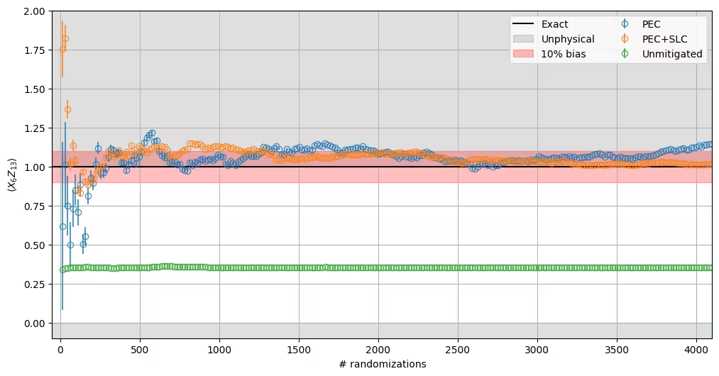
จากการตรวจสอบผลการทดลอง เราสามารถเปรียบเทียบพฤติกรรมของแนวทางต่างๆ ได้โดยตรง ได้แก่ PEC, PEC ที่รวมกับ SLC และ baseline ที่ไม่ได้ลด error รายละเอียดเฉพาะที่ควรเน้น:
-
ผลลัพธ์ที่ไม่ได้ลด error อยู่นอกแถบ bias 10% อย่างมาก (ใกล้ 0.35) และไม่ได้รับผลกระทบจากจำนวนการสุ่ม
-
บนอุปกรณ์นี้ PEC เต็มรูปแบบมี sampling overhead ที่ หลังจากการแกว่งตัวขนาดใหญ่ในช่วงแรก ค่าประมาณ plain-PEC จะกู้คืนสัญญาณและลู่เข้าสู่ประมาณ 1.1 ซึ่งเกินค่าที่แท้จริงเล็กน้อย โปรดทราบว่าแถบ bias 10% ใช้ได้กับ estimator ของ PEC+SLC เท่านั้น: plain PEC โดยหลักการแล้วไม่มี bias ดังนั้นค่าเบี่ยงเบนที่เหลืออยู่นี้จึงไม่ได้อยู่ภายใต้การรับประกัน bias แต่สะท้อนถึงความผันผวนทางสถิติและความไม่สมบูรณ์แบบใน noise model ที่เรียนรู้มา ซึ่งถือว่าสมเหตุสมผลสำหรับปัญหาขนาดนี้
-
SLC ลด overhead ลงอีกประมาณ 3.4 เท่า (เหลือ สำหรับขอบเขต residual-bias ที่ประมาณ 10%) PEC+SLC ก็ผันผวนอย่างมากที่จำนวนการสุ่มน้อย โดยในช่วงแรกถึงกับเข้าสู่บริเวณที่ไม่เป็นไปตามหลักฟิสิกส์ แต่ค่าประมาณของมันบรรจบเข้าสู่ค่าที่แท้จริงอย่างสม่ำเสมอ โดยลู่เข้าสู่ใกล้ 1.0 ซึ่งอยู่ลึกเข้าไปในแถบ มันมีความแม่นยำเทียบเท่าหรือดีกว่า plain PEC ด้วยต้นทุนการสุ่มเพียงประมาณหนึ่งในสาม ซึ่งแสดงให้เห็นถึงประโยชน์ของ lightcone shading
-
error bar ของค่าประมาณที่ลด error ทั้งสองแบบจะหดตัวลงเมื่อการสุ่มสะสมมากขึ้น เมื่อจำนวนการสุ่มคงที่ estimator ของ PEC+SLC จะมีความแปรปรวนทางสถิติที่เล็กกว่า ซึ่งสอดคล้องกับค่า ที่เล็กกว่า
โปรดทราบว่าอัตรา noise ที่เรียนรู้มา (และดังนั้นทั้ง overhead และค่าประมาณที่ลด error) ขึ้นอยู่กับ backend และการปรับเทียบ ณ เวลาที่รัน ดังนั้นการรัน notebook นี้ซ้ำอาจให้ค่าที่แตกต่างกันในเชิงปริมาณ
fig, ax = plt.subplots(1, 1, figsize=(12, 6))

ax.axhline(1.0, color="black", label="Exact")
ax.fill_between(
    [-50, 4100], -10, 0, color="grey", alpha=0.25, label="Unphysical"
)
ax.fill_between([-50, 4100], 1, 10, color="grey", alpha=0.25)
ax.fill_between(
    [-50, 4100], 0.9, 1.1, color="red", alpha=0.25, label="10% bias"
)

for label, res in results.items():
    ax.errorbar(
        list(range(steps, num_randomizations + 1, steps)),
        [r[0] for r in res],
        yerr=[r[1] for r in res],
        alpha=0.75,
        marker="o",
        linestyle="",
        markerfacecolor="none",
        label=label,
    )

ax.set_ylabel(r"$\langle X_{6}Z_{13}\rangle$")
ax.set_xlabel("# randomizations")
ax.grid()

ax.legend(ncols=2)
ax.set_ylim([-0.1, 2.0])
ax.set_xlim([-50, 4100])
(-50.0, 4100.0)
ขั้นตอนถัดไป
หากคุณพบว่างานนี้น่าสนใจ คุณอาจสนใจเนื้อหาต่อไปนี้: