Performance Management: Qiskit Function โดย Q-CTRL Fire Opal
Qiskit Functions เป็นฟีเจอร์ทดลองที่ให้บริการเฉพาะผู้ใช้ IBM Quantum® Premium Plan, Flex Plan, และ On-Prem (ผ่าน IBM Quantum Platform API) Plan เท่านั้น อยู่ในสถานะ preview release และอาจมีการเปลี่ยนแปลงได้
Package versions
โค้ดในหน้านี้ได้รับการพัฒนาโดยใช้ requirement ดังต่อไปนี้ เราแนะนำให้ใช้เวอร์ชันเหล่านี้หรือใหม่กว่า
qiskit[all]~=2.3.1
qiskit-ibm-runtime~=0.45.1
ภาพรวม
Fire Opal Performance Management ทำให้ทุกคนสามารถดึงผลลัพธ์ที่มีความหมายจากคอมพิวเตอร์ควอนตัมในระดับขนาดใหญ่ได้อย่างง่ายดาย โดยไม่ต้องเป็นผู้เชี่ยวชาญด้านฮาร์ดแวร์ควอนตัม เมื่อรัน Circuit กับ Fire Opal Performance Management เทคนิคการระงับข้อผิดพลาดแบบ AI-driven จะถูกนำมาใช้โดยอัตโนมัติ ทำให้สามารถขยายขนาดปัญหาที่ใช้ Gate และ Qubit จำนวนมากขึ้นได้ วิธีนี้ลดจำนวน shot ที่ต้องการเพื่อให้ได้คำตอบที่ถูกต้อง โดยไม่มี overhead เพิ่มเติม ส่งผลให้ประหยัดทั้งเวลาประมวลผลและค่าใช้จ่ายได้อย่างมีนัยสำคัญ
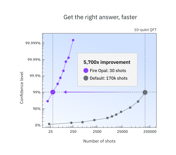
Performance Management ระงับข้อผิดพลาดและเพิ่มความน่าจะเป็นในการได้คำตอบที่ถูกต้องบนฮาร์ดแวร์ที่มีสัญญาณรบกวน กล่าวคือมันเพิ่มอัตราส่วนสัญญาณต่อสัญญาณรบกวน ภาพต่อไปนี้แสดงให้เห็นว่าความแม่นยำที่เพิ่มขึ้นจาก Performance Management ช่วยลดความจำเป็นในการใช้ shot เพิ่มเติมได้อย่างไร ในกรณีของอัลกอริทึม Quantum Fourier Transform ขนาด 10 Qubit ด้วย shot เพียง 30 ครั้ง Q-CTRL สามารถถึงเกณฑ์ความเชื่อมั่น 99% ในขณะที่ค่าเริ่มต้น (QiskitRuntime Sampler, optimization_level=3 และ resilience_level=1, ibm_sherbrooke) ต้องการถึง 170,000 shot การได้คำตอบที่ถูกต้องเร็วขึ้นช่วยประหยัดเวลาประมวลผลได้มาก
ฟังก์ชัน Performance Management สามารถใช้กับอัลกอริทึมใดก็ได้ และใช้แทน IBM Quantum primitives มาตรฐานได้อย่างง่ายดาย เบื้องหลังมีเทคนิคการระงับข้อผิดพลาดหลายอย่างทำงานร่วมกันเพื่อป้องกันข้อผิดพลาดไม่ให้เกิดขึ้นในขณะรัน เมธอด pipeline ทั้งหมดของ Fire Opal ถูกตั้งค่าล่วงหน้าและไม่ขึ้นกับอัลกอริทึม หมายความว่าคุณจะได้ประสิทธิภาพดีที่สุดทันทีโดยไม่ต้องตั้งค่าเพิ่มเติม
หากต้องการเข้าถึง Performance Management ติดต่อ Q-CTRL
คำอธิบาย
Fire Opal Performance Management มีสองตัวเลือกสำหรับการประมวลผลที่คล้ายกับ IBM Quantum primitives ทำให้สามารถสลับไปใช้ Q-CTRL Sampler และ Estimator ได้อย่างง่ายดาย ขั้นตอนทั่วไปในการใช้ฟังก์ชัน Performance Management คือ:
- กำหนด Circuit ของคุณ (และ operators ในกรณีของ Estimator)
- รัน Circuit
- ดึงผลลัพธ์
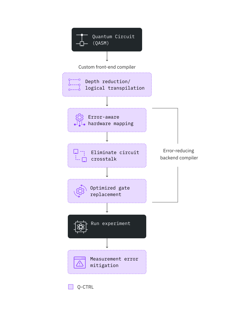
เพื่อลดสัญญาณรบกวนของฮาร์ดแวร์ Fire Opal ใช้เทคนิคการระงับข้อผิดพลาดแบบ AI-driven หลายอย่างตามที่แสดงในภาพต่อไปนี้ เมื่อใช้ Fire Opal pipeline ทั้งหมดถูกทำให้เป็นอัตโนมัติอย่างสมบูรณ์โดยไม่ต้องตั้งค่าใดๆ
pipeline ของ Fire Opal ขจัดความจำเป็นต้องใช้ overhead เพิ่มเติม เช่น เวลา quantum runtime ที่เพิ่มขึ้น หรือ physical Qubit พิเศษ โปรดทราบว่าเวลาประมวลผลแบบ classical ยังคงเป็นปัจจัย (ดูส่วน Benchmarks สำหรับการประมาณ โดย "Total time" สะท้อนทั้งการประมวลผลแบบ classical และ quantum) ต่างจาก error mitigation ที่ต้องใช้ overhead ในรูปแบบของการสุ่มตัวอย่าง การระงับข้อผิดพลาดของ Fire Opal ทำงานทั้งในระดับ Gate และ pulse เพื่อจัดการกับแหล่งที่มาของสัญญาณรบกวนต่างๆ และป้องกันความน่าจะเป็นที่จะเกิดข้อผิดพลาด การป้องกันข้อผิดพลาดทำให้ไม่ต้องทำ post-processing ที่มีต้นทุนสูง
ภาพต่อไปนี้แสดงวิธีการระงับข้อผิดพลาดที่ทำงานโดยอัตโนมัติใน Fire Opal Performance Management
ฟังก์ชันนี้มี primitives สองตัวคือ Sampler และ Estimator โดยอินพุตและเอาต์พุตของทั้งสองขยายสเปค IBM Quantum V2 primitives
Benchmarks
ผลการ benchmarking แบบ algorithmic ที่เผยแพร่แล้ว แสดงให้เห็นการปรับปรุงประสิทธิภาพอย่างมีนัยสำคัญในอัลกอริทึมต่างๆ รวมถึง Bernstein-Vazirani, quantum Fourier transform, การค้นหาของ Grover, quantum approximate optimization algorithm, และ variational quantum eigensolver ส่วนที่เหลือของส่วนนี้ให้รายละเอียดเพิ่มเติมเกี่ยวกับประเภทของอัลกอริทึมที่คุณรันได้ รวมถึงประสิทธิภาพและรันไทม์ที่คาดหวัง
การศึกษาอิสระต่อไปนี้แสดงให้เห็นว่า Performance Management ของ Q-CTRL ช่วยให้ทำงานวิจัยเชิงอัลกอริทึมในระดับที่ทำลายสถิติได้:
- Parametrized Energy-Efficient Quantum Kernels for Network Service Fault Diagnosis - quantum kernel learning สูงสุด 50 Qubit
- Tensor-based quantum phase difference estimation for large-scale demonstration - quantum phase estimation สูงสุด 33 Qubit
- Hierarchical Learning for Quantum ML: Novel Training Technique for Large-Scale Variational Quantum Circuits - quantum data loading สูงสุด 21 Qubit
ตารางต่อไปนี้ให้แนวทางคร่าวๆ เกี่ยวกับความแม่นยำและรันไทม์จากการรัน benchmarking ก่อนหน้าบน ibm_fez ประสิทธิภาพบนอุปกรณ์อื่นอาจแตกต่างกัน เวลาการใช้งานอ้างอิงจากสมมติฐาน 10,000 shot ต่อ Circuit "จำนวน Qubit" ที่ระบุไม่ใช่ข้อจำกัดแบบเด็ดขาด แต่แสดงถึงเกณฑ์คร่าวๆ ที่คาดว่าจะได้ความแม่นยำของคำตอบที่สม่ำเสมออย่างมาก ปัญหาที่มีขนาดใหญ่กว่าได้รับการแก้ไขสำเร็จแล้ว และขอแนะนำให้ทดสอบเกินขีดจำกัดเหล่านี้
| ตัวอย่าง | จำนวน Qubit | ความแม่นยำ | ตัวชี้วัดความแม่นยำ | เวลารวม (วินาที) | การใช้งาน Runtime (วินาที) | Primitive (Mode) |
|---|---|---|---|---|---|---|
| Bernstein–Vazirani | 50Q | 100% | Success Rate (เปอร์เซ็นต์ของการรันที่คำตอบที่ถูกต้องมีจำนวนนับสูงสุด) | 10 | 8 | Sampler |
| Quantum Fourier Transform | 30Q | 100% | Success Rate (เปอร์เซ็นต์ของการรันที่คำตอบที่ถูกต้องมีจำนวนนับสูงสุด) | 10 | 8 | Sampler |
| Quantum Phase Estimation | 30Q | 99.9998% | ความแม่นยำของมุมที่พบ: 1- abs(real_angle - angle_found)/pi | 10 | 8 | Sampler |
| Quantum simulation: Ising model (15 steps) | 20Q | 99.775% | (นิยามด้านล่าง) | 60 (ต่อ step) | 15 (ต่อ step) | Estimator |
| Quantum simulation 2: molecular dynamics (20 time points) | 34Q | 96.78% | (นิยามด้านล่าง) | 10 (ต่อจุดเวลา) | 6 (ต่อจุดเวลา) | Estimator |
การกำหนดความแม่นยำของการวัด expectation value - เมตริก นิยามดังนี้:
โดยที่ = expectation value ในอุดมคติ, = expectation value ที่วัดได้, = ค่าสูงสุดในอุดมคติ, และ = ค่าต่ำสุดในอุดมคติ คือค่าเฉลี่ยของ จากการวัดหลายครั้ง
เมตริกนี้ถูกใช้เพราะไม่เปลี่ยนแปลงเมื่อช่วงของค่าที่เป็นไปได้ถูกเลื่อนหรือปรับสเกลทั้งช่วง กล่าวคือไม่ว่าคุณจะเลื่อนช่วงของ expectation value ที่เป็นไปได้ขึ้นหรือลง หรือเพิ่มการกระจาย ค่าของ ก็ควรคงที่
เริ่มต้นใช้งาน
Fire Opal Performance Management ใช้ Qiskit v2.0.0 ซึ่งเป็นเวอร์ชันที่แนะนำ เวอร์ชันที่รองรับคือ Qiskit >=v2.0.0
Authenticate โดยใช้ IBM Quantum Platform API key และเลือก Qiskit Function ดังนี้ (snippet นี้สมมติว่าคุณได้ บันทึกบัญชีของคุณ ไว้ในสภาพแวดล้อมท้องถิ่นแล้ว)
# Added by doQumentation — required packages for this notebook
!pip install -q matplotlib numpy qiskit qiskit-ibm-catalog qiskit-ibm-runtime
# This cell is hidden from users. It hides the "...You have imported samplomatic..." warning.
import warnings

warnings.filterwarnings("ignore", message=".*You have imported samplomatic*")
from qiskit_ibm_catalog import QiskitFunctionsCatalog

catalog = QiskitFunctionsCatalog(channel="ibm_quantum_platform")

# verify that you have access to the function
catalog.list()
[QiskitFunction(qunova/hivqe-chemistry),
 QiskitFunction(global-data-quantum/quantum-portfolio-optimizer),
 QiskitFunction(algorithmiq/tem),
 QiskitFunction(qedma/qesem),
 QiskitFunction(multiverse/singularity),
 QiskitFunction(ibm/circuit-function),
 QiskitFunction(q-ctrl/optimization-solver),
 QiskitFunction(colibritd/quick-pde),
 QiskitFunction(q-ctrl/performance-management),
 QiskitFunction(kipu-quantum/iskay-quantum-optimizer)]
# Access Function
perf_mgmt = catalog.load("q-ctrl/performance-management")
หากต้องการใช้ Backend ที่ฟังก์ชันนี้ยังไม่รองรับในขณะนี้ ติดต่อ Q-CTRL เพื่อขอเพิ่มการรองรับ
พรีมิทีฟ Estimator
ตัวอย่าง Estimator
ใช้ Estimator primitive ของ Fire Opal Performance Management เพื่อหา expectation value ของคู่ Circuit-observable เดียว
นอกจากแพ็คเกจ qiskit-ibm-catalog และ qiskit แล้ว คุณจะใช้แพ็คเกจ numpy ด้วยในการรันตัวอย่างนี้ คุณสามารถติดตั้งแพ็คเกจนี้โดยยกเลิกคอมเมนต์ใน cell ต่อไปนี้หากรันตัวอย่างใน notebook ที่ใช้ IPython kernel
# %pip install numpy
1. สร้าง Circuit
ในตัวอย่างนี้ สร้าง Hermitian operator แบบสุ่มและ observable เพื่อใส่เข้าไปในฟังก์ชัน Performance Management
import numpy as np
from qiskit.circuit.library import iqp
from qiskit.quantum_info import random_hermitian, SparsePauliOp

n_qubits = 50

# Generate a random circuit
mat = np.real(random_hermitian(n_qubits, seed=1234))
circuit = iqp(mat)
circuit.measure_all()

# Define observables as a string
observable = SparsePauliOp("Z" * n_qubits)
# Create PUB tuple
estimator_pubs = [(circuit, observable)]
2. รัน Circuit
รัน Circuit และกำหนด Backend และจำนวน shot ตามต้องการ
# This cell is hidden from users
from qiskit_ibm_runtime import QiskitRuntimeService

service = QiskitRuntimeService()
backend_name = service.least_busy().name
# Run the circuit using Estimator
qctrl_estimator_job = perf_mgmt.run(
    primitive="estimator",
    pubs=estimator_pubs,
    backend_name=backend_name,
)
คุณสามารถใช้ Qiskit Serverless APIs ที่คุ้นเคยเพื่อตรวจสอบสถานะของ Qiskit Function workload:
qctrl_estimator_job.status()
'QUEUED'
3. ดึงผลลัพธ์
# Retrieve the counts from the result list
result = qctrl_estimator_job.result()
ผลลัพธ์มีรูปแบบเดียวกับ Estimator result:
import numpy

result_str = str(result)

with numpy.printoptions(threshold=200):
    print(
        f"The result of the submitted job had {len(result)} PUB "
        f"and has a value:\n {result[0]}\n"
    )

print("The associated PubResult of this job has the following DataBins:")
print(f"{result[0].data}\n")

print(f"And this DataBin has attributes: {result[0].data.keys()}")

print("The expectation values measured from this PUB are:")
print(f"{result[0].data.evs}")
The result of the submitted job had 1 PUB
The result of the submitted job had 1 PUB and has a value:
 PubResult(data=DataBin(evs=0.0195, stds=0.9998098569228051), metadata={'precision': None})

The associated PubResult of this job has the following DataBins:
DataBin(evs=0.0195, stds=0.9998098569228051)

And this DataBin has attributes: dict_keys(['evs', 'stds'])
The expectation values measured from this PUB are:
0.0195
พรีมิทีฟ Sampler
ตัวอย่าง Sampler
ใช้ Sampler primitive ของ Fire Opal Performance Management เพื่อรัน Bernstein–Vazirani circuit อัลกอริทึมนี้ใช้สำหรับค้นหา hidden string จาก output ของฟังก์ชัน black box และเป็นอัลกอริทึม benchmarking ที่นิยมใช้กันเพราะมีคำตอบที่ถูกต้องเพียงคำตอบเดียว 1. สร้าง Circuit
กำหนดคำตอบที่ถูกต้องของอัลกอริทึม ซึ่งก็คือ hidden bitstring และ Bernstein–Vazirani circuit ปรับความกว้างของ Circuit ได้โดยแค่เปลี่ยนค่า circuit_width
import qiskit

circuit_width = 35
hidden_bitstring = "1" * circuit_width

# Create circuit, reserving one qubit for BV oracle
bv_circuit = qiskit.QuantumCircuit(circuit_width + 1, circuit_width)
bv_circuit.x(circuit_width)
bv_circuit.h(range(circuit_width + 1))
for input_qubit, bit in enumerate(reversed(hidden_bitstring)):
    if bit == "1":
        bv_circuit.cx(input_qubit, circuit_width)
bv_circuit.barrier()
bv_circuit.h(range(circuit_width + 1))
bv_circuit.barrier()
for input_qubit in range(circuit_width):
    bv_circuit.measure(input_qubit, input_qubit)

# Create PUB tuple
sampler_pubs = [(bv_circuit,)]
2. รัน Circuit
รัน Circuit และกำหนด Backend และจำนวน shot ตามต้องการ
# Run the circuit using Sampler
qctrl_sampler_job = perf_mgmt.run(
    primitive="sampler",
    pubs=sampler_pubs,
    backend_name=backend_name,
)
ตรวจสอบ สถานะ ของ Qiskit Function workload หรือดึง ผลลัพธ์ ดังนี้:
# Print the ID so you can use it later, if necessary
print(qctrl_sampler_job.job_id)

qctrl_sampler_job.status()
60fe2fa1-a860-43e4-8615-c6ac4180f93b
'QUEUED'
3. ดึงผลลัพธ์
# Retrieve the job results
sampler_result = qctrl_sampler_job.result()
# Get results for the first (and only) PUB
pub_result = sampler_result[0]
counts = pub_result.data.c.get_counts()

print("Counts for the meas output register (limited to 30 results):")
for i, (bitstring, count) in enumerate(counts.items()):
    if i >= 50:
        print(f"  ... ({len(counts) - 30} more items)")
        break
    print(f"  {bitstring}: {count}")
Counts for the meas output register (limited to 30 results):
  11111111111111111111111111111111111: 1661
  11111111111111111111111111110111111: 60
  11111111111111111111111111111101111: 54
  11111111111111111111111111111110111: 54
  11111111111111011111111111111111111: 46
  11111111111111111110111111111111111: 44
  11111111111111111111111101111111111: 42
  11111111111111111111111110111111111: 42
  11111111111111110111111111111111111: 41
  11111111111111111111111111111111101: 39
  11111111111111111111101111111111111: 38
  11111111111111111111110111111111111: 38
  11111111111111111111111111101111111: 37
  11111111111111111111111111111111110: 36
  11111111111110111111111111111111111: 35
  11111111111111111111111111111011111: 32
  11111111111111101111111111111111111: 32
  01111111111111111111111111111111111: 27
  11111111111111111011111111111111111: 23
  11111111101111111111111111111111111: 22
  11111111111111111111111111111111011: 21
  11111111011111111111111111111111111: 20
  00000000000000011111111111111111111: 18
  11111111111111111111110101111111111: 18
  00000001111111111111111111111111111: 17
  11111111001111111111111111111111111: 16
  11101111111111111111111111111111111: 16
  11111111111101111111111111111111111: 16
  00000101111111111111111111111111111: 13
  11111111111111111111111011111111111: 13
  11111111111111111111111110101111111: 13
  11111111111111111101111111111111111: 12
  10111111111111111111111111111111111: 12
  11111111111111111111111110001111111: 12
  00000000000000000011111111111111111: 11
  11111111111111111111111111111110110: 10
  00000000000000000000000001111111111: 10
  11111111111011111111111111111111111: 9
  11111111111111101011111111111111111: 9
  00000000011111111111111111111111111: 8
  10101111111111111111111111111111111: 8
  00000000000000000000000001011111111: 8
  11111111111111111111111111111111001: 8
  00000111111111111111111111111111111: 7
  11111111111111111111111111111101110: 7
  11111111110111111111111111111111111: 7
  00000000000001011111111111111111111: 6
  00000000000000001111111111111111111: 6
  00000000000000000001011111111111111: 6
  11111111111111111111111111011111111: 6
  ... (1050 more items)
3. พล็อต bitstring ที่มี count สูงสุด
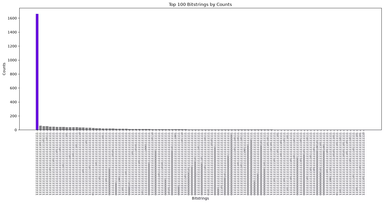
พล็อต bitstring ที่มี count สูงสุดเพื่อดูว่า hidden bitstring เป็น mode หรือเปล่า
import matplotlib.pyplot as plt

def plot_top_bitstrings(counts_dict, hidden_bitstring=None):
    # Sort and take the top 100 bitstrings
    top_100 = sorted(counts_dict.items(), key=lambda x: x[1], reverse=True)[
        :100
    ]
    if not top_100:
        print("No bitstrings found in the input dictionary.")
        return

    # Unzip the bitstrings and their counts
    bitstrings, counts = zip(*top_100)

    # Assign colors: purple if the bitstring matches hidden_bitstring,
    # otherwise gray
    colors = [
        "#680CE9" if bit == hidden_bitstring else "gray" for bit in bitstrings
    ]

    # Create the bar plot
    plt.figure(figsize=(15, 8))
    plt.bar(
        range(len(bitstrings)), counts, tick_label=bitstrings, color=colors
    )

    # Rotate the bitstrings for better readability
    plt.xticks(rotation=90, fontsize=8)
    plt.xlabel("Bitstrings")
    plt.ylabel("Counts")
    plt.title("Top 100 Bitstrings by Counts")

    # Show the plot
    plt.tight_layout()
    plt.show()
hidden bitstring จะถูกเน้นด้วยสีม่วง และควรเป็น bitstring ที่มีจำนวน count สูงสุด
plot_top_bitstrings(counts, hidden_bitstring)
Changelog
-
2026-02-20: ประกาศการเลิกใช้งาน - ฟิลด์ metadata
provider_job_idsจะถูกเลิกใช้งานใน 30 วันในเวอร์ชัน 0.13.0 ผู้ใช้สามารถเข้าถึง job ID ผ่านเมธอดjob_id()ของ runtime service -
2026-02-11: ขณะนี้รองรับ
ibm_miamiแล้ว และเพิ่ม execution metadata ในPubResult
รับการสนับสนุน
สำหรับคำถามหรือปัญหาใด ๆ ติดต่อ Q-CTRL
ขั้นตอนถัดไป
-
ขอสิทธิ์เข้าถึง Q-CTRL Performance Management.
-
เยี่ยมชม API reference สำหรับ Qiskit Function นี้
-
ลองทำ tutorial Transverse-Field Ising Model with Q-CTRL's Performance Management
-
ลองทำ tutorial Quantum Phase Estimation with Q-CTRL's Qiskit Functions
-
ทบทวน Redacted bank case study.
-
ทบทวน BlueQubit case study