Transverse-Field Ising Model กับ Performance Management ของ Q-CTRL

ประมาณการใช้งาน: 2 นาทีบนโปรเซสเซอร์ Heron r2 (หมายเหตุ: นี่เป็นเพียงการประมาณเท่านั้น เวลาจริงอาจแตกต่างกันได้)

พื้นหลัง

Transverse-Field Ising Model (TFIM) มีความสำคัญในการศึกษาแม่เหล็กควอนตัมและการเปลี่ยนเฟส โมเดลนี้อธิบายชุดของสปินที่จัดเรียงบนโครงตาข่าย โดยแต่ละสปินจะโต้ตอบกับสปินข้างเคียงพร้อมกับได้รับอิทธิพลจากสนามแม่เหล็กภายนอกที่ขับเคลื่อนความผันผวนเชิงควอนตัม

แนวทางทั่วไปในการจำลองโมเดลนี้คือการใช้ Trotter decomposition เพื่อประมาณตัวดำเนินการ time evolution ซึ่งสร้าง Circuit ที่สลับกันระหว่าง single-qubit rotation กับ entangling two-qubit interaction อย่างไรก็ตาม การจำลองบนฮาร์ดแวร์จริงเป็นเรื่องท้าทายเนื่องจากเสียงรบกวนและ decoherence ซึ่งทำให้ผลลัพธ์เบี่ยงเบนจากไดนามิกที่แท้จริง เพื่อแก้ปัญหานี้ เราใช้เครื่องมือ error suppression และ performance management ของ Q-CTRL ที่ชื่อว่า Fire Opal ซึ่งมีให้บริการในรูปแบบ Qiskit Function (ดู เอกสาร Fire Opal) Fire Opal ปรับแต่งการรัน Circuit อัตโนมัติโดยใช้ dynamical decoupling, advanced layout, routing และเทคนิค error suppression อื่น ๆ เพื่อลดเสียงรบกวน ด้วยการปรับปรุงเหล่านี้ ผลลัพธ์จากฮาร์ดแวร์จึงใกล้เคียงกับการจำลองแบบไม่มีเสียงรบกวนมากขึ้น ทำให้เราสามารถศึกษาไดนามิกของ TFIM magnetization ได้อย่างแม่นยำยิ่งขึ้น

ในบทเรียนนี้เราจะ:

• สร้าง TFIM Hamiltonian บนกราฟของ spin triangle ที่เชื่อมต่อกัน
• จำลอง time evolution ด้วย Trotterized Circuit ที่ความลึกต่าง ๆ
• คำนวณและแสดงผล single-qubit magnetization $\langle Z_i \rangle$ ตามเวลา
• เปรียบเทียบการจำลองแบบพื้นฐานกับผลลัพธ์จากการรันบนฮาร์ดแวร์โดยใช้ Fire Opal performance management ของ Q-CTRL

ภาพรวม

Transverse-field Ising Model (TFIM) เป็นโมเดลสปินควอนตัมที่จับลักษณะสำคัญของการเปลี่ยนเฟสควอนตัม Hamiltonian ถูกนิยามดังนี้:

$$H = -J \sum_{i} Z_i Z_{i+1} - h \sum_{i} X_i$$

โดยที่ $Z_i$ และ $X_i$ คือตัวดำเนินการ Pauli ที่กระทำบน Qubit $i$, $J$ คือความแข็งแกร่งของการเชื่อมต่อระหว่างสปินที่อยู่ติดกัน และ $h$ คือความแรงของสนามแม่เหล็กตามขวาง พจน์แรกแทนการโต้ตอบแบบ ferromagnetic แบบคลาสสิก ส่วนพจน์ที่สองแนะนำความผันผวนเชิงควอนตัมผ่านสนามตามขวาง ในการจำลองไดนามิกของ TFIM เราใช้ Trotter decomposition ของตัวดำเนินการ unitary evolution $e^{-iHt}$ ซึ่งนำไปใช้งานผ่านชั้นของ Gate RX และ RZZ ที่อิงกับกราฟสปิน triangle แบบกำหนดเอง การจำลองนี้สำรวจว่า magnetization $\langle Z \rangle$ วิวัฒน์อย่างไรเมื่อจำนวน Trotter step เพิ่มขึ้น

ประสิทธิภาพของการนำ TFIM ไปใช้งานนี้ถูกประเมินโดยเปรียบเทียบการจำลองแบบไม่มีเสียงรบกวนกับ Backend ที่มีเสียงรบกวน ฟีเจอร์ enhanced execution และ error suppression ของ Fire Opal ถูกนำมาใช้เพื่อลดผลกระทบของเสียงรบกวนในฮาร์ดแวร์จริง ทำให้ได้ค่าประมาณของ spin observable เช่น $\langle Z_i \rangle$ และ correlator $\langle Z_i Z_j \rangle$ ที่น่าเชื่อถือยิ่งขึ้น

ข้อกำหนด

ก่อนเริ่มบทเรียนนี้ ให้ตรวจสอบว่าได้ติดตั้งสิ่งต่อไปนี้แล้ว:

• Qiskit SDK v1.4 หรือใหม่กว่า พร้อมรองรับ visualization
• Qiskit Runtime v0.40 หรือใหม่กว่า (pip install qiskit-ibm-runtime)
• Qiskit Functions Catalog v0.9.0 (pip install qiskit-ibm-catalog)
• Fire Opal SDK v9.0.2 หรือใหม่กว่า (pip install fire-opal)
• Q-CTRL Visualizer v8.0.2 หรือใหม่กว่า (pip install qctrl-visualizer)

ตั้งค่า

ขั้นแรก ยืนยันตัวตนด้วย IBM Quantum API key ของคุณ จากนั้นเลือก Qiskit Function ดังนี้ (โค้ดนี้สมมติว่าคุณได้ บันทึกบัญชีของคุณ ไว้ในสภาพแวดล้อมท้องถิ่นแล้ว)

# Added by doQumentation — required packages for this notebook
!pip install -q matplotlib networkx numpy qctrlvisualizer qiskit qiskit-aer qiskit-ibm-catalog qiskit-ibm-runtime

from qiskit.transpiler.preset_passmanagers import generate_preset_pass_manager
from qiskit import QuantumCircuit
from qiskit_ibm_catalog import QiskitFunctionsCatalog
from qiskit_ibm_runtime import QiskitRuntimeService
from qiskit_ibm_runtime import SamplerV2 as Sampler
from qiskit.quantum_info import SparsePauliOp
from qiskit_aer import AerSimulator

import numpy as np
import networkx as nx
import matplotlib.pyplot as plt
import qctrlvisualizer as qv

catalog = QiskitFunctionsCatalog(channel="ibm_quantum_platform")

# Access Function
perf_mgmt = catalog.load("q-ctrl/performance-management")

ขั้นตอนที่ 1: แมปอินพุตแบบคลาสสิกไปยังปัญหาควอนตัม

สร้างกราฟ TFIM

เราเริ่มต้นด้วยการกำหนดโครงตาข่ายของสปินและการเชื่อมต่อระหว่างกัน ในบทเรียนนี้ โครงตาข่ายถูกสร้างจาก triangle ที่เชื่อมต่อกันเรียงเป็นห่วงโซ่เชิงเส้น แต่ละ triangle ประกอบด้วยโหนดสามโหนดที่เชื่อมกันเป็นวงปิด และห่วงโซ่ถูกสร้างโดยเชื่อมต่อโหนดหนึ่งของแต่ละ triangle กับ triangle ก่อนหน้า

ฟังก์ชันช่วยเหลือ connected_triangles_adj_matrix สร้าง adjacency matrix สำหรับโครงสร้างนี้ สำหรับห่วงโซ่ของ $n$ triangle กราฟที่ได้จะมี $2n+1$ โหนด

def connected_triangles_adj_matrix(n):
    """
    Generate the adjacency matrix for 'n' connected triangles in a chain.
    """
    num_nodes = 2 * n + 1
    adj_matrix = np.zeros((num_nodes, num_nodes), dtype=int)

    for i in range(n):
        a, b, c = i * 2, i * 2 + 1, i * 2 + 2  # Nodes of the current triangle

        # Connect the three nodes in a triangle
        adj_matrix[a, b] = adj_matrix[b, a] = 1
        adj_matrix[b, c] = adj_matrix[c, b] = 1
        adj_matrix[a, c] = adj_matrix[c, a] = 1

        # If not the first triangle, connect to the previous triangle
        if i > 0:
            adj_matrix[a, a - 1] = adj_matrix[a - 1, a] = 1

    return adj_matrix

เพื่อแสดงโครงตาข่ายที่เราเพิ่งกำหนด เราสามารถพล็อตห่วงโซ่ของ triangle ที่เชื่อมต่อกันและระบุชื่อแต่ละโหนด ฟังก์ชันด้านล่างสร้างกราฟสำหรับจำนวน triangle ที่เลือกและแสดงผล

def plot_triangle_chain(n, side=1.0):
    """
    Plot a horizontal chain of n equilateral triangles.
    Baseline: even nodes (0,2,4,...,2n) on y=0
    Apexes: odd nodes (1,3,5,...,2n-1) above the midpoint.
    """
    # Build graph
    A = connected_triangles_adj_matrix(n)
    G = nx.from_numpy_array(A)

    h = np.sqrt(3) / 2 * side
    pos = {}

    # Place baseline nodes
    for k in range(n + 1):
        pos[2 * k] = (k * side, 0.0)

    # Place apex nodes
    for k in range(n):
        x_left = pos[2 * k][0]
        x_right = pos[2 * k + 2][0]
        pos[2 * k + 1] = ((x_left + x_right) / 2, h)

    # Draw
    fig, ax = plt.subplots(figsize=(1.5 * n, 2.5))
    nx.draw(
        G,
        pos,
        ax=ax,
        with_labels=True,
        font_size=10,
        font_color="white",
        node_size=600,
        node_color=qv.QCTRL_STYLE_COLORS[0],
        edge_color="black",
        width=2,
    )
    ax.set_aspect("equal")
    ax.margins(0.2)
    plt.show()

    return G, pos

สำหรับบทเรียนนี้ เราจะใช้ห่วงโซ่ของ triangle จำนวน 20 อัน

n_triangles = 20
n_qubits = 2 * n_triangles + 1
plot_triangle_chain(n_triangles, side=1.0)
plt.show()

การระบายสีขอบกราฟ

เพื่อนำ spin-spin coupling ไปใช้งาน มีประโยชน์มากในการจัดกลุ่มขอบที่ไม่ทับซ้อนกัน ซึ่งช่วยให้เราสามารถใช้ two-qubit Gate แบบขนานได้ เราทำได้ด้วยขั้นตอนการระบายสีขอบแบบง่าย [1] ซึ่งกำหนดสีให้กับแต่ละขอบเพื่อให้ขอบที่พบกันที่โหนดเดียวกันอยู่ในกลุ่มที่ต่างกัน

def edge_coloring(graph):
    """
    Takes a NetworkX graph and returns a list of lists where each inner list contains
    the edges assigned the same color.
    """
    line_graph = nx.line_graph(graph)
    edge_colors = nx.coloring.greedy_color(line_graph)

    color_groups = {}
    for edge, color in edge_colors.items():
        if color not in color_groups:
            color_groups[color] = []
        color_groups[color].append(edge)

    return list(color_groups.values())

ขั้นตอนที่ 2: ปรับแต่งปัญหาสำหรับการรันบนฮาร์ดแวร์ควอนตัม

สร้าง Trotterized Circuit บนกราฟสปิน

เพื่อจำลองไดนามิกของ TFIM เราสร้าง Circuit ที่ประมาณตัวดำเนินการ time evolution

$$U(t) = e^{-i H t}, \quad \text{where} \quad H = -J \sum_{\langle i,j \rangle} Z_i Z_j - h \sum_i X_i .$$

เราใช้ second-order Trotter decomposition:

$$e^{-i H \Delta t} \approx e^{-i H_X \Delta t / 2}\, e^{-i H_Z \Delta t}\, e^{-i H_X \Delta t / 2},$$

โดยที่ $H_X = -h \sum_i X_i$ และ $H_Z = -J \sum_{\langle i,j \rangle} Z_i Z_j$

• พจน์ $H_X$ นำไปใช้งานด้วยชั้นของ RX rotation
• พจน์ $H_Z$ นำไปใช้งานด้วยชั้นของ Gate RZZ ตามขอบของกราฟการโต้ตอบ

มุมของ Gate เหล่านี้ถูกกำหนดโดย transverse field $h$, coupling constant $J$ และ time step $\Delta t$ การซ้อน Trotter step หลาย ๆ ชั้นทำให้เราสร้าง Circuit ที่มีความลึกเพิ่มขึ้นซึ่งประมาณไดนามิกของระบบ ฟังก์ชัน generate_tfim_circ_custom_graph และ trotter_circuits สร้าง Trotterized quantum Circuit จากกราฟการโต้ตอบสปินแบบใดก็ได้

def generate_tfim_circ_custom_graph(
    steps, h, J, dt, psi0, graph: nx.graph.Graph, meas_basis="Z", mirror=False
):
    """
    Generate a second order trotter of the form e^(a+b) ~ e^(b/2) e^a e^(b/2) for simulating a transverse field ising model:
    e^{-i H t} where the Hamiltonian H = -J \\sum_i Z_i Z_{i+1} + h \\sum_i X_i.

    steps: Number of trotter steps
    theta_x: Angle for layer of X rotations
    theta_zz: Angle for layer of ZZ rotations
    theta_x: Angle for second layer of X rotations
    J: Coupling between nearest neighbor spins
    h: The transverse magnetic field strength
    dt: t/total_steps
    psi0: initial state (assumed to be prepared in the computational basis).
    meas_basis: basis to measure all correlators in

    This is a second order trotter of the form e^(a+b) ~ e^(b/2) e^a e^(b/2)
    """
    theta_x = h * dt
    theta_zz = -2 * J * dt
    nq = graph.number_of_nodes()
    color_edges = edge_coloring(graph)
    circ = QuantumCircuit(nq, nq)
    # Initial state, for typical cases in the computational basis
    for i, b in enumerate(psi0):
        if b == "1":
            circ.x(i)
    # Trotter steps
    for step in range(steps):
        for i in range(nq):
            circ.rx(theta_x, i)
        if mirror:
            color_edges = [sublist[::-1] for sublist in color_edges[::-1]]
        for edge_list in color_edges:
            for edge in edge_list:
                circ.rzz(theta_zz, edge[0], edge[1])
        for i in range(nq):
            circ.rx(theta_x, i)

    # some typically used basis rotations
    if meas_basis == "X":
        for b in range(nq):
            circ.h(b)
    elif meas_basis == "Y":
        for b in range(nq):
            circ.sdg(b)
            circ.h(b)

    for i in range(nq):
        circ.measure(i, i)

    return circ

def trotter_circuits(G, d_ind_tot, J, h, dt, meas_basis, mirror=True):
    """
    Generates a sequence of Trotterized circuits, each with increasing depth.
    Given a spin interaction graph and Hamiltonian parameters, it constructs
    a list of circuits with 1 to d_ind_tot Trotter steps

    G: Graph defining spin interactions (edges = ZZ couplings)
    d_ind_tot: Number of Trotter steps (maximum depth)
    J: Coupling between nearest neighboring spins
    h: Transverse magnetic field strength
    dt: (t / total_steps
    meas_basis: Basis to measure all correlators in
    mirror: If True, mirror the Trotter layers
    """
    qubit_count = len(G)
    circuits = []
    psi0 = "0" * qubit_count

    for steps in range(1, d_ind_tot + 1):
        circuits.append(
            generate_tfim_circ_custom_graph(
                steps, h, J, dt, psi0, G, meas_basis, mirror
            )
        )
    return circuits

ประมาณค่า single-qubit magnetization $\langle Z_i \rangle$

เพื่อศึกษาไดนามิกของโมเดล เราต้องการวัด magnetization ของแต่ละ Qubit ซึ่งกำหนดโดยค่าคาดหวัง $\langle Z_i \rangle = \langle \psi | Z_i | \psi \rangle$

ในการจำลอง เราสามารถคำนวณได้โดยตรงจากผลลัพธ์การวัด ฟังก์ชัน z_expectation ประมวลผลจำนวน bitstring และส่งคืนค่า $\langle Z_i \rangle$ สำหรับดัชนี Qubit ที่เลือก บนฮาร์ดแวร์จริง เราประเมินค่าเดียวกันโดยระบุตัวดำเนินการ Pauli โดยใช้ฟังก์ชัน generate_z_observables จากนั้น Backend จะคำนวณค่าคาดหวัง

def z_expectation(counts, index):
    """
    counts: Dict of mitigated bitstrings.
    index: Index i in the single operator expectation value < II...Z_i...I > to be calculated.
    return:  < Z_i >
    """
    z_exp = 0
    tot = 0
    for bitstring, value in counts.items():
        bit = int(bitstring[index])
        sign = 1
        if bit % 2 == 1:
            sign = -1
        z_exp += sign * value
        tot += value

    return z_exp / tot

def generate_z_observables(nq):
    observables = []
    for i in range(nq):
        pauli_string = "".join(["Z" if j == i else "I" for j in range(nq)])
        observables.append(SparsePauliOp(pauli_string))
    return observables

observables = generate_z_observables(n_qubits)

ตอนนี้เรากำหนดพารามิเตอร์สำหรับการสร้าง Trotterized Circuit ในบทเรียนนี้ โครงตาข่ายเป็นห่วงโซ่ของ triangle ที่เชื่อมต่อกัน 20 อัน ซึ่งตรงกับระบบ 41-Qubit

all_circs_mirror = []
for num_triangles in [n_triangles]:
    for meas_basis in ["Z"]:
        A = connected_triangles_adj_matrix(num_triangles)
        G = nx.from_numpy_array(A)
        nq = len(G)
        d_ind_tot = 22
        dt = 2 * np.pi * 1 / 30 * 0.25
        J = 1
        h = -7
        all_circs_mirror.extend(
            trotter_circuits(G, d_ind_tot, J, h, dt, meas_basis, True)
        )
circs = all_circs_mirror

ขั้นตอนที่ 3: รันด้วย Qiskit primitives

รัน MPS simulation

รายการ Circuit แบบ Trotterized จะถูกรันด้วย simulator matrix_product_state โดยใช้จำนวน $4096$ shots ตามที่กำหนดไว้ วิธี MPS ให้การประมาณค่าพลศาสตร์ของ Circuit ที่มีประสิทธิภาพ โดยความแม่นยำขึ้นอยู่กับ bond dimension ที่เลือก สำหรับขนาดระบบที่พิจารณาในที่นี้ bond dimension ค่าเริ่มต้นเพียงพอสำหรับจับพลศาสตร์ค่า magnetization ด้วยความเที่ยงตรงสูง raw counts จะถูก normalize แล้วนำมาคำนวณค่าคาดหวังของ Qubit เดี่ยว $\langle Z_i \rangle$ ในแต่ละ Trotter step สุดท้ายเราคำนวณค่าเฉลี่ยของ Qubit ทั้งหมดเพื่อได้เส้นโค้งเดี่ยวที่แสดงการเปลี่ยนแปลงของค่า magnetization ตามเวลา

backend_sim = AerSimulator(method="matrix_product_state")

def normalize_counts(counts_list, shots):
    new_counts_list = []
    for counts in counts_list:
        a = {k: v / shots for k, v in counts.items()}
        new_counts_list.append(a)
    return new_counts_list

def run_sim(circ_list):
    shots = 4096
    res = backend_sim.run(circ_list, shots=shots)
    normed = normalize_counts(res.result().get_counts(), shots)
    return normed

sim_counts = run_sim(circs)

รันบน hardware

service = QiskitRuntimeService()
backend = service.backend("ibm_marrakesh")

def run_qiskit(circ_list):
    shots = 4096
    pm = generate_preset_pass_manager(backend=backend)
    isa_circuits = [pm.run(qc) for qc in circ_list]
    sampler = Sampler(mode=backend)
    res = sampler.run(isa_circuits, shots=shots)
    res = [r.data.c.get_counts() for r in res.result()]
    normed = normalize_counts(res, shots)
    return normed

qiskit_counts = run_qiskit(circs)

รันบน hardware ด้วย Fire Opal

เราประเมินพลศาสตร์ค่า magnetization บน quantum hardware จริง Fire Opal มี Qiskit Function ที่ขยายความสามารถของ Estimator primitive มาตรฐานของ Qiskit Runtime ด้วยการกำจัด error อัตโนมัติและการจัดการประสิทธิภาพ เราส่ง Circuit แบบ Trotterized โดยตรงไปยัง Backend ของ IBM® ขณะที่ Fire Opal จัดการการรันที่คำนึงถึง noise

เราเตรียมรายการ pubs โดยแต่ละรายการมี Circuit และ observable Pauli-Z ที่สอดคล้องกัน สิ่งเหล่านี้จะถูกส่งไปยัง estimator function ของ Fire Opal ซึ่งคืนค่าคาดหวัง $\langle Z_i \rangle$ สำหรับแต่ละ Qubit ในแต่ละ Trotter step จากนั้นสามารถเฉลี่ยผลลัพธ์ข้าม Qubit เพื่อได้เส้นโค้ง magnetization จาก hardware

backend_name = "ibm_marrakesh"
estimator_pubs = [(qc, observables) for qc in all_circs_mirror[:]]

# Run the circuit using the estimator
qctrl_estimator_job = perf_mgmt.run(
    primitive="estimator",
    pubs=estimator_pubs,
    backend_name=backend_name,
    options={"default_shots": 4096},
)

result_qctrl = qctrl_estimator_job.result()

ขั้นตอนที่ 4: ประมวลผลภายหลังและคืนผลลัพธ์ในรูปแบบ classical ที่ต้องการ

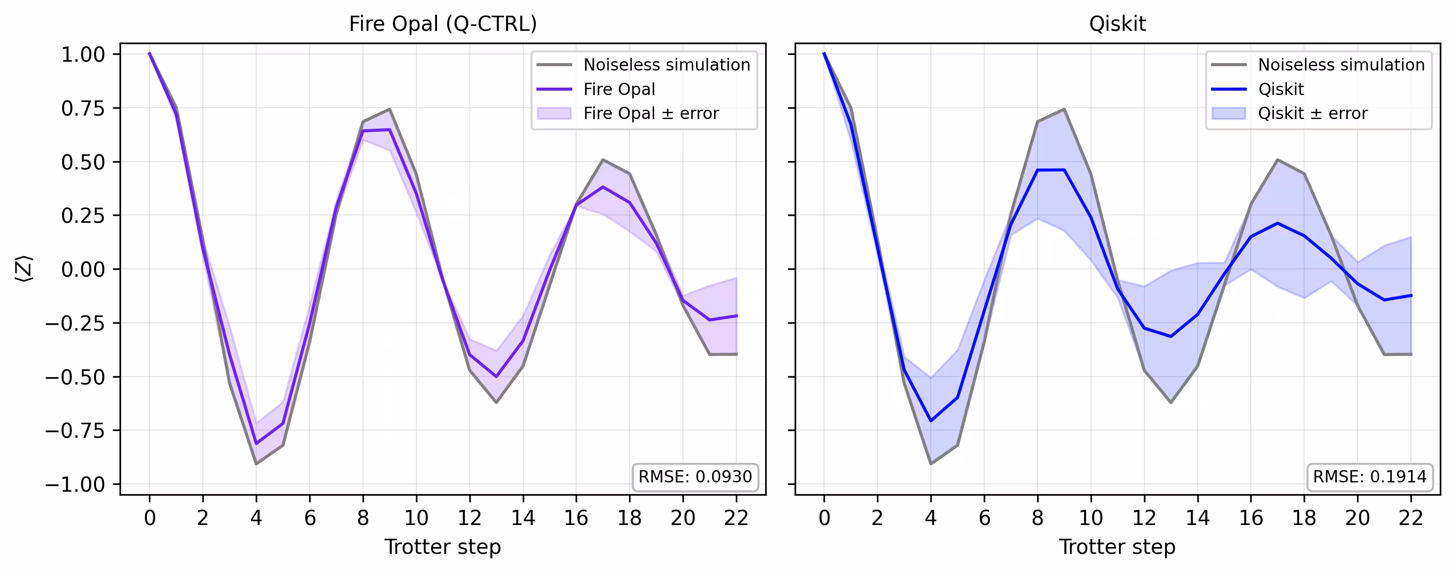
สุดท้าย เราเปรียบเทียบเส้นโค้ง magnetization จาก simulator กับผลลัพธ์ที่ได้จาก hardware จริง การพล็อตทั้งสองไว้ด้วยกันแสดงให้เห็นว่าการรันบน hardware ด้วย Fire Opal ใกล้เคียงกับ baseline ที่ไม่มี noise ตลอด Trotter step มากแค่ไหน

def make_correlators(test_counts, nq, d_ind_tot):
    mz = np.empty((nq, d_ind_tot))
    for d_ind in range(d_ind_tot):
        counts = test_counts[d_ind]
        for i in range(nq):
            mz[i, d_ind] = z_expectation(counts, i)
    average_z = np.mean(mz, axis=0)
    return np.concatenate((np.array([1]), average_z), axis=0)

sim_exp = make_correlators(sim_counts[0:22], nq=nq, d_ind_tot=22)
qiskit_exp = make_correlators(qiskit_counts[0:22], nq=nq, d_ind_tot=22)

qctrl_exp = [ev.data.evs for ev in result_qctrl[:]]
qctrl_exp_mean = np.concatenate(
    (np.array([1]), np.mean(qctrl_exp, axis=1)), axis=0
)

def make_expectations_plot(
    sim_z,
    depths,
    exp_qctrl=None,
    exp_qctrl_error=None,
    exp_qiskit=None,
    exp_qiskit_error=None,
    plot_from=0,
    plot_upto=23,
):
    import numpy as np
    import matplotlib.pyplot as plt

    depth_ticks = [0, 2, 4, 6, 8, 10, 12, 14, 16, 18, 20, 22]

    d = np.asarray(depths)[plot_from:plot_upto]
    sim = np.asarray(sim_z)[plot_from:plot_upto]

    qk = (
        None
        if exp_qiskit is None
        else np.asarray(exp_qiskit)[plot_from:plot_upto]
    )
    qc = (
        None
        if exp_qctrl is None
        else np.asarray(exp_qctrl)[plot_from:plot_upto]
    )

    qk_err = (
        None
        if exp_qiskit_error is None
        else np.asarray(exp_qiskit_error)[plot_from:plot_upto]
    )
    qc_err = (
        None
        if exp_qctrl_error is None
        else np.asarray(exp_qctrl_error)[plot_from:plot_upto]
    )

    # ---- helper(s) ----
    def rmse(a, b):
        if a is None or b is None:
            return None
        a = np.asarray(a, dtype=float)
        b = np.asarray(b, dtype=float)
        mask = np.isfinite(a) & np.isfinite(b)
        if not np.any(mask):
            return None
        diff = a[mask] - b[mask]
        return float(np.sqrt(np.mean(diff**2)))

    def plot_panel(ax, method_y, method_err, color, label, band_color=None):
        # Noiseless reference
        ax.plot(d, sim, color="grey", label="Noiseless simulation")

        # Method line + band
        if method_y is not None:
            ax.plot(d, method_y, color=color, label=label)
            if method_err is not None:
                lo = np.clip(method_y - method_err, -1.05, 1.05)
                hi = np.clip(method_y + method_err, -1.05, 1.05)
                ax.fill_between(
                    d,
                    lo,
                    hi,
                    alpha=0.18,
                    color=band_color if band_color else color,
                    label=f"{label} ± error",
                )
        else:
            ax.text(
                0.5,
                0.5,
                "No data",
                transform=ax.transAxes,
                ha="center",
                va="center",
                fontsize=10,
                color="0.4",
            )

        # RMSE box (vs sim)
        r = rmse(method_y, sim)
        if r is not None:
            ax.text(
                0.98,
                0.02,
                f"RMSE: {r:.4f}",
                transform=ax.transAxes,
                va="bottom",
                ha="right",
                fontsize=8,
                bbox=dict(
                    boxstyle="round,pad=0.35", fc="white", ec="0.7", alpha=0.9
                ),
            )
        # Axes
        ax.set_xticks(depth_ticks)
        ax.set_ylim(-1.05, 1.05)
        ax.grid(True, which="both", linewidth=0.4, alpha=0.4)
        ax.set_axisbelow(True)
        ax.legend(prop={"size": 8}, loc="best")

    fig, axes = plt.subplots(1, 2, figsize=(10, 4), dpi=300, sharey=True)

    axes[0].set_title("Fire Opal (Q-CTRL)", fontsize=10)
    plot_panel(
        axes[0],
        qc,
        qc_err,
        color="#680CE9",
        label="Fire Opal",
        band_color="#680CE9",
    )
    axes[0].set_xlabel("Trotter step")
    axes[0].set_ylabel(r"$\langle Z \rangle$")
    axes[1].set_title("Qiskit", fontsize=10)
    plot_panel(
        axes[1], qk, qk_err, color="blue", label="Qiskit", band_color="blue"
    )
    axes[1].set_xlabel("Trotter step")

    plt.tight_layout()
    plt.show()

depths = list(range(d_ind_tot + 1))
errors = np.abs(np.array(qctrl_exp_mean) - np.array(sim_exp))

errors_qiskit = np.abs(np.array(qiskit_exp) - np.array(sim_exp))

make_expectations_plot(
    sim_exp,
    depths,
    exp_qctrl=qctrl_exp_mean,
    exp_qctrl_error=errors,
    exp_qiskit=qiskit_exp,
    exp_qiskit_error=errors_qiskit,
)

อ้างอิง

[1] Graph coloring. Wikipedia. Retrieved September 15, 2025, from https://en.wikipedia.org/wiki/Graph_coloring

แบบสำรวจ tutorial

Link to survey

Note: This survey is provided by IBM Quantum and relates to the original English content. To give feedback on doQumentation's website, translations, or code execution, please open a GitHub issue.

กรุณาใช้เวลาสักครู่เพื่อให้ feedback เกี่ยวกับ tutorial นี้ ความคิดเห็นของคุณจะช่วยให้เราปรับปรุงเนื้อหาและประสบการณ์การใช้งาน