Quantum Phase Estimation ด้วย Qiskit Functions ของ Q-CTRL

ประมาณการใช้งาน: 40 วินาที บน Heron r2 processor (หมายเหตุ: นี่เป็นการประมาณการเท่านั้น เวลาจริงอาจแตกต่างกันได้)

พื้นฐาน

Quantum Phase Estimation (QPE) เป็น algorithm พื้นฐานในการคำนวณแบบควอนตัม ที่เป็นรากฐานของแอปพลิเคชันสำคัญหลายอย่าง เช่น Shor's algorithm, การประมาณพลังงาน ground-state ในเคมีควอนตัม และปัญหา eigenvalue QPE จะประมาณค่า phase $\varphi$ ที่สัมพันธ์กับ eigenstate ของ unitary operator ซึ่งเข้ารหัสไว้ในความสัมพันธ์

$U \lvert \varphi \rangle = e^{2\pi i \varphi} \lvert \varphi \rangle,$

และหาค่านั้นด้วยความแม่นยำ $\epsilon = O(1/2^m)$ โดยใช้ counting qubits จำนวน $m$ ตัว [1] ด้วยการเตรียม qubits เหล่านี้ใน superposition, ใช้ controlled powers ของ $U$, แล้วใช้ inverse Quantum Fourier Transform (QFT) เพื่อดึง phase ออกมาเป็นผลลัพธ์การวัดที่เข้ารหัสแบบ binary QPE จะสร้าง probability distribution ที่กระจุกตัวอยู่ที่ bitstrings ซึ่งเศษส่วน binary ใกล้เคียงกับ $\varphi$ ในกรณีอุดมคติ ผลลัพธ์การวัดที่น่าจะเป็นที่สุดจะตรงกับการขยาย binary ของ phase โดยตรง ส่วนความน่าจะเป็นของผลลัพธ์อื่นจะลดลงอย่างรวดเร็วตามจำนวน counting qubits อย่างไรก็ตาม การรัน QPE circuit ที่ลึกบน hardware จริงมีความท้าทาย: จำนวน qubits มากและการดำเนินการ entangling ทำให้ algorithm ไวต่อ decoherence และ gate error อย่างมาก ส่งผลให้การกระจาย bitstring กว้างขึ้นและเลื่อนออกไป ทำให้บดบัง eigenphase ที่แท้จริง และ bitstring ที่มีความน่าจะเป็นสูงสุดอาจไม่ตรงกับการขยาย binary ที่ถูกต้องของ $\varphi$ อีกต่อไป

ใน tutorial นี้ เราจะนำเสนอการใช้งาน QPE algorithm โดยใช้เครื่องมือ error suppression และ performance management ของ Q-CTRL อย่าง Fire Opal ซึ่งมีให้ใช้งานในรูป Qiskit Function (ดู เอกสาร Fire Opal) Fire Opal จะใช้การปรับแต่งขั้นสูงโดยอัตโนมัติ ทั้ง dynamical decoupling, การปรับปรุง qubit layout และเทคนิค error suppression ส่งผลให้ได้ผลลัพธ์ที่มีความเที่ยงตรงสูงขึ้น ซึ่งทำให้การกระจาย bitstring บน hardware ใกล้เคียงกับที่ได้จาก simulation แบบ noiseless มากขึ้น จนสามารถระบุ eigenphase ที่ถูกต้องได้อย่างน่าเชื่อถือแม้มี noise

ข้อกำหนด

ก่อนเริ่ม tutorial นี้ ให้แน่ใจว่าคุณติดตั้งสิ่งต่อไปนี้แล้ว:

• Qiskit SDK v1.4 ขึ้นไป พร้อม visualization support
• Qiskit Runtime v0.40 ขึ้นไป (pip install qiskit-ibm-runtime)
• Qiskit Functions Catalog v0.9.0 (pip install qiskit-ibm-catalog)
• Fire Opal SDK v9.0.2 ขึ้นไป (pip install fire-opal)
• Q-CTRL Visualizer v8.0.2 ขึ้นไป (pip install qctrl-visualizer)

การตั้งค่า

ก่อนอื่น ยืนยันตัวตนด้วย IBM Quantum API key ของคุณ จากนั้นเลือก Qiskit Function ดังนี้ (โค้ดนี้สมมติว่าคุณบันทึก account ไปยัง local environment แล้ว)

# Added by doQumentation — required packages for this notebook
!pip install -q matplotlib numpy qctrlvisualizer qiskit qiskit-aer qiskit-ibm-catalog qiskit-ibm-runtime

from qiskit import QuantumCircuit

import numpy as np
import matplotlib.pyplot as plt
import qiskit
from qiskit import qasm2
from qiskit_aer import AerSimulator
from qiskit_ibm_runtime import QiskitRuntimeService
from qiskit_ibm_runtime import SamplerV2 as Sampler
from qiskit.transpiler.preset_passmanagers import generate_preset_pass_manager
import qctrlvisualizer as qv
from qiskit_ibm_catalog import QiskitFunctionsCatalog

plt.style.use(qv.get_qctrl_style())

catalog = QiskitFunctionsCatalog(channel="ibm_quantum_platform")

# Access Function
perf_mgmt = catalog.load("q-ctrl/performance-management")

ขั้นตอนที่ 1: แปลง input แบบ classical ไปเป็นปัญหาควอนตัม

ใน tutorial นี้ เราจะสาธิต QPE เพื่อกู้คืน eigenphase ของ unitary แบบ single-qubit ที่รู้ค่าอยู่แล้ว unitary ที่เราต้องการประมาณ phase ของมันคือ single-qubit phase gate ที่ใช้กับ target qubit:

$$U(\theta)= \begin{pmatrix} 1 & 0\\[2pt] 0 & e^{i\theta} \end{pmatrix} = e^{i\theta\,|1\rangle\!\langle 1|}.$$

เราเตรียม eigenstate $|\psi\rangle=|1\rangle$ ของมัน เนื่องจาก $|1\rangle$ เป็น eigenvector ของ $U(\theta)$ ที่มี eigenvalue $e^{i\theta}$ ดังนั้น eigenphase ที่ต้องการประมาณคือ:

$$\varphi = \frac{\theta}{2\pi} \pmod{1}$$

เราตั้งค่า $\theta=\tfrac{1}{6}\cdot 2\pi$ ดังนั้น ground-truth phase คือ $\varphi=1/6$ QPE circuit จะใช้งาน controlled powers $U^{2^k}$ โดยใช้ controlled phase rotation ที่มีมุม $\theta\cdot2^k$ จากนั้นใช้ inverse QFT กับ counting register แล้ววัดค่า bitstrings ที่ได้จะกระจุกตัวอยู่รอบ ๆ binary representation ของ $1/6$

Circuit ใช้ counting qubits จำนวน $m$ ตัว (เพื่อกำหนดความแม่นยำของการประมาณ) บวกกับ target qubit อีก 1 ตัว เริ่มด้วยการกำหนด building block ที่จำเป็นสำหรับ QPE ได้แก่ Quantum Fourier Transform (QFT) และ inverse ของมัน, utility function สำหรับแปลงระหว่าง decimal กับ binary fraction ของ eigenphase และ helper สำหรับ normalize raw counts เป็น probability เพื่อเปรียบเทียบผลลัพธ์จาก simulation กับ hardware

def inverse_quantum_fourier_transform(quantum_circuit, number_of_qubits):
    """
    Apply an inverse Quantum Fourier Transform the first `number_of_qubits` qubits in the
    `quantum_circuit`.
    """
    for qubit in range(number_of_qubits // 2):
        quantum_circuit.swap(qubit, number_of_qubits - qubit - 1)
    for j in range(number_of_qubits):
        for m in range(j):
            quantum_circuit.cp(-np.pi / float(2 ** (j - m)), m, j)
        quantum_circuit.h(j)
    return quantum_circuit

def bitstring_count_to_probabilities(data, shot_count):
    """
    This function turns an unsorted dictionary of bitstring counts into a sorted dictionary
    of probabilities.
    """
    # Turn the bitstring counts into probabilities.
    probabilities = {
        bitstring: bitstring_count / shot_count
        for bitstring, bitstring_count in data.items()
    }

    sorted_probabilities = dict(
        sorted(probabilities.items(), key=lambda x: x[1], reverse=True)
    )

    return sorted_probabilities

ขั้นตอนที่ 2: ปรับแต่งปัญหาสำหรับการรันบน quantum hardware

เราสร้าง QPE circuit โดยเตรียม counting qubits ใน superposition, ใช้ controlled phase rotation เพื่อเข้ารหัส target eigenphase และจบด้วย inverse QFT ก่อนทำการวัด

def quantum_phase_estimation_benchmark_circuit(
    number_of_counting_qubits, phase
):
    """
    Create the circuit for quantum phase estimation.

    Parameters
    ----------
    number_of_counting_qubits : The number of qubits in the circuit.
    phase : The desired phase.

    Returns
    -------
    QuantumCircuit
        The quantum phase estimation circuit for `number_of_counting_qubits` qubits.
    """
    qc = QuantumCircuit(
        number_of_counting_qubits + 1, number_of_counting_qubits
    )
    target = number_of_counting_qubits

    # |1> eigenstate for the single-qubit phase gate
    qc.x(target)

    # Hadamards on counting register
    for q in range(number_of_counting_qubits):
        qc.h(q)

    # ONE controlled phase per counting qubit: cp(phase * 2**k)
    for k in range(number_of_counting_qubits):
        qc.cp(phase * (1 << k), k, target)

    qc.barrier()

    # Inverse QFT on counting register
    inverse_quantum_fourier_transform(qc, number_of_counting_qubits)

    qc.barrier()
    for q in range(number_of_counting_qubits):
        qc.measure(q, q)
    return qc

ขั้นตอนที่ 3: รันด้วย Qiskit primitives

เราตั้งค่าจำนวน shot และ qubit สำหรับการทดลอง และเข้ารหัส target phase $\varphi = 1/6$ โดยใช้ binary digits จำนวน $m$ ตัว ด้วย parameter เหล่านี้ เราสร้าง QPE circuit ที่จะรันบน simulation, hardware แบบ default และ backend ที่ใช้ Fire Opal

shot_count = 10000
num_qubits = 35
phase = (1 / 6) * 2 * np.pi
circuits_quantum_phase_estimation = (
    quantum_phase_estimation_benchmark_circuit(
        number_of_counting_qubits=num_qubits, phase=phase
    )
)

รัน MPS simulation

ก่อนอื่น เราสร้าง reference distribution โดยใช้ matrix_product_state simulator แล้วแปลง counts เป็น normalized probability เพื่อใช้เปรียบเทียบกับผลลัพธ์จาก hardware ในภายหลัง

# Run the algorithm on the IBM Aer simulator.
aer_simulator = AerSimulator(method="matrix_product_state")

# Transpile the circuits for the simulator.
transpiled_circuits = qiskit.transpile(
    circuits_quantum_phase_estimation, aer_simulator
)

simulated_result = (
    aer_simulator.run(transpiled_circuits, shots=shot_count)
    .result()
    .get_counts()
)

simulated_result_probabilities = []

simulated_result_probabilities.append(
    bitstring_count_to_probabilities(
        simulated_result,
        shot_count=shot_count,
    )
)

รันบน hardware

service = QiskitRuntimeService()
backend = service.least_busy(operational=True, simulator=False)

pm = generate_preset_pass_manager(backend=backend, optimization_level=3)
isa_circuits = pm.run(circuits_quantum_phase_estimation)

# Run the algorithm with IBM default.
sampler = Sampler(backend)

# Run all circuits using Qiskit Runtime.
ibm_default_job = sampler.run([isa_circuits], shots=shot_count)

รันบน hardware ด้วย Fire Opal

# Run the circuit using the sampler
fire_opal_job = perf_mgmt.run(
    primitive="sampler",
    pubs=[qasm2.dumps(circuits_quantum_phase_estimation)],
    backend_name=backend.name,
    options={"default_shots": shot_count},
)

ขั้นตอนที่ 4: ประมวลผลและแสดงผลลัพธ์ในรูปแบบ classical ที่ต้องการ

# Retrieve results.
ibm_default_result = ibm_default_job.result()
ibm_default_probabilities = []

for idx, pub_result in enumerate(ibm_default_result):
    ibm_default_probabilities.append(
        bitstring_count_to_probabilities(
            pub_result.data.c0.get_counts(),
            shot_count=shot_count,
        )
    )

fire_opal_result = fire_opal_job.result()

fire_opal_probabilities = []
for idx, pub_result in enumerate(fire_opal_result):
    fire_opal_probabilities.append(
        bitstring_count_to_probabilities(
            pub_result.data.c0.get_counts(),
            shot_count=shot_count,
        )
    )

data = {
    "simulation": simulated_result_probabilities,
    "default": ibm_default_probabilities,
    "fire_opal": fire_opal_probabilities,
}

def plot_distributions(
    data,
    number_of_counting_qubits,
    top_k=None,
    by="prob",
    shot_count=None,
):
    def nrm(d):
        s = sum(d.values())
        return {k: (v / s if s else 0.0) for k, v in d.items()}

    def as_float(d):
        return {k: float(v) for k, v in d.items()}

    def to_space(d):
        if by == "prob":
            return nrm(as_float(d))
        else:
            if shot_count and 0.99 <= sum(d.values()) <= 1.01:
                return {
                    k: v * float(shot_count) for k, v in as_float(d).items()
                }
            else:
                return as_float(d)

    def topk(d, k):
        items = sorted(d.items(), key=lambda kv: kv[1], reverse=True)
        return items[: (k or len(d))]

    phase = "1/6"

    sim = to_space(data["simulation"])
    dft = to_space(data["default"])
    qct = to_space(data["fire_opal"])

    correct = max(sim, key=sim.get) if sim else None
    print("Correct result:", correct)

    sim_items = topk(sim, top_k)
    dft_items = topk(dft, top_k)
    qct_items = topk(qct, top_k)

    sim_keys, y_sim = zip(*sim_items) if sim_items else ([], [])
    dft_keys, y_dft = zip(*dft_items) if dft_items else ([], [])
    qct_keys, y_qct = zip(*qct_items) if qct_items else ([], [])

    fig, axes = plt.subplots(3, 1, layout="constrained")
    ylab = "Probabilities"

    def panel(ax, keys, ys, title, color):
        x = np.arange(len(keys))
        bars = ax.bar(x, ys, color=color)
        ax.set_title(title)
        ax.set_ylabel(ylab)
        ax.set_xticks(x)
        ax.set_xticklabels(keys, rotation=90)
        ax.set_xlabel("Bitstrings")
        if correct in keys:
            i = keys.index(correct)
            bars[i].set_edgecolor("black")
            bars[i].set_linewidth(2)
        return max(ys, default=0.0)

    c_sim, c_dft, c_qct = (
        qv.QCTRL_STYLE_COLORS[5],
        qv.QCTRL_STYLE_COLORS[1],
        qv.QCTRL_STYLE_COLORS[0],
    )
    m1 = panel(axes[0], list(sim_keys), list(y_sim), "Simulation", c_sim)
    m2 = panel(axes[1], list(dft_keys), list(y_dft), "Default", c_dft)
    m3 = panel(axes[2], list(qct_keys), list(y_qct), "Q-CTRL", c_qct)

    for ax, m in zip(axes, (m1, m2, m3)):
        ax.set_ylim(0, 1.05 * (m or 1.0))

    for ax in axes:
        ax.label_outer()
    fig.suptitle(
        rf"{number_of_counting_qubits} counting qubits, $2\pi\varphi$={phase}"
    )
    fig.set_size_inches(20, 10)
    plt.show()

experiment_index = 0
phase_index = 0

distributions = {
    "simulation": data["simulation"][phase_index],
    "default": data["default"][phase_index],
    "fire_opal": data["fire_opal"][phase_index],
}

plot_distributions(
    distributions, num_qubits, top_k=100, by="prob", shot_count=shot_count
)

Correct result: 00101010101010101010101010101010101

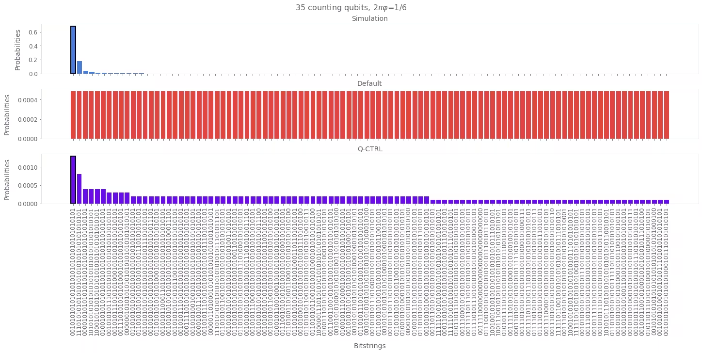
Simulation ทำหน้าที่เป็น baseline สำหรับ eigenphase ที่ถูกต้อง การรันบน hardware แบบ default แสดงให้เห็น noise ที่บดบังผลลัพธ์นี้ เนื่องจาก noise กระจาย probability ไปยัง bitstrings ที่ไม่ถูกต้องจำนวนมาก แต่ด้วย Q-CTRL Performance Management การกระจายจะคมชัดขึ้นและกู้คืนผลลัพธ์ที่ถูกต้องได้ ทำให้ QPE ในขนาดนี้น่าเชื่อถือ

อ้างอิง

[1] Lecture 7: Phase Estimation and Factoring. IBM Quantum Learning - Fundamentals of quantum algorithms. Retrieved October 3, 2025.

แบบสำรวจ Tutorial

ขอเชิญสละเวลาสักครู่เพื่อให้ feedback เกี่ยวกับ tutorial นี้ ความคิดเห็นของคุณจะช่วยให้เราพัฒนาเนื้อหาและประสบการณ์การใช้งานได้ดียิ่งขึ้น

ลิงก์ไปยังแบบสำรวจ

Note: This survey is provided by IBM Quantum and relates to the original English content. To give feedback on doQumentation's website, translations, or code execution, please open a GitHub issue.