ตัวอย่างและการประยุกต์ใช้

ในบทเรียนนี้ เราจะสำรวจตัวอย่าง variational algorithm และวิธีนำไปใช้:

• วิธีเขียน variational algorithm แบบกำหนดเอง
• วิธีนำ variational algorithm ไปหาค่า eigenvalue ต่ำสุด
• วิธีนำ variational algorithm ไปใช้แก้ปัญหาในการประยุกต์จริง

สังเกตว่า Qiskit patterns framework สามารถนำไปใช้กับทุกปัญหาที่เราแนะนำในที่นี้ อย่างไรก็ตาม เพื่อหลีกเลี่ยงความซ้ำซ้อน เราจะระบุขั้นตอนของ framework อย่างชัดเจนเฉพาะในตัวอย่างเดียว ที่รันบน hardware จริง

นิยามปัญหา

สมมติว่าเราต้องการใช้ variational algorithm หาค่า eigenvalue ของ observable ต่อไปนี้:

$$\hat{O}_1 = 2 II - 2 XX + 3 YY - 3 ZZ,$$

observable นี้มีค่า eigenvalue ดังนี้:

$$\left\{ \begin{array}{c} \lambda_0 = -6 \\ \lambda_1 = 4 \\ \lambda_2 = 4 \\ \lambda_3 = 6 \end{array} \right\}$$

และ eigenstate:

$$\left\{ \begin{array}{c} |\phi_0\rangle = \frac{1}{\sqrt{2}}(|00\rangle + |11\rangle)\\ |\phi_1\rangle = \frac{1}{\sqrt{2}}(|00\rangle - |11\rangle)\\ |\phi_2\rangle = \frac{1}{\sqrt{2}}(|01\rangle - |10\rangle)\\ |\phi_3\rangle = \frac{1}{\sqrt{2}}(|01\rangle + |10\rangle) \end{array} \right\}$$

# Added by doQumentation — required packages for this notebook
!pip install -q numpy qiskit qiskit-ibm-runtime rustworkx scipy

from qiskit.quantum_info import SparsePauliOp

observable_1 = SparsePauliOp.from_list([("II", 2), ("XX", -2), ("YY", 3), ("ZZ", -3)])

Custom VQE

เราจะสำรวจวิธีสร้าง VQE instance ด้วยตัวเองก่อน เพื่อหาค่า eigenvalue ต่ำสุดของ $\hat{O}_1$ ซึ่งจะรวมเทคนิคหลากหลายที่เราเรียนมาตลอดคอร์สนี้

def cost_func_vqe(params, ansatz, hamiltonian, estimator):
    """Return estimate of energy from estimator

    Parameters:
        params (ndarray): Array of ansatz parameters
        ansatz (QuantumCircuit): Parameterized ansatz circuit
        hamiltonian (SparsePauliOp): Operator representation of Hamiltonian
        estimator (Estimator): Estimator primitive instance

    Returns:
        float: Energy estimate
    """
    pub = (ansatz, hamiltonian, params)
    cost = estimator.run([pub]).result()[0].data.evs

    return cost

from qiskit.circuit.library.n_local import n_local
from qiskit import QuantumCircuit

import numpy as np

reference_circuit = QuantumCircuit(2)
reference_circuit.x(0)

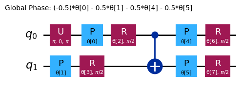
variational_form = n_local(
    num_qubits=2,
    rotation_blocks=["rz", "ry"],
    entanglement_blocks="cx",
    entanglement="linear",
    reps=1,
)

raw_ansatz = reference_circuit.compose(variational_form)
raw_ansatz.decompose().draw("mpl")

เราจะเริ่ม debug บน local simulator ก่อน

from qiskit.primitives import StatevectorEstimator as Estimator
from qiskit.primitives import StatevectorSampler as Sampler

estimator = Estimator()
sampler = Sampler()

ตอนนี้เราตั้งค่า parameter เริ่มต้น:

x0 = np.ones(raw_ansatz.num_parameters)
print(x0)

[1. 1. 1. 1. 1. 1. 1. 1.]

เราสามารถ minimize cost function นี้เพื่อคำนวณ parameter ที่เหมาะสมที่สุด

# SciPy minimizer routine
from scipy.optimize import minimize
import time

start_time = time.time()

result = minimize(
    cost_func_vqe,
    x0,
    args=(raw_ansatz, observable_1, estimator),
    method="COBYLA",
    options={"maxiter": 1000, "disp": True},
)

end_time = time.time()
execution_time = end_time - start_time

Return from COBYLA because the trust region radius reaches its lower bound.
Number of function values = 103   Least value of F = -5.999999998357189
The corresponding X is:
[2.27483579e+00 8.37593091e-01 1.57080508e+00 5.82932911e-06
 2.49973063e+00 6.41884255e-01 6.33686904e-01 6.33688223e-01]

result

message: Return from COBYLA because the trust region radius reaches its lower bound.
 success: True
  status: 0
     fun: -5.999999998357189
       x: [ 2.275e+00  8.376e-01  1.571e+00  5.829e-06  2.500e+00
            6.419e-01  6.337e-01  6.337e-01]
    nfev: 103
   maxcv: 0.0

เนื่องจากปัญหาทดสอบนี้ใช้แค่ 2 Qubit เราสามารถตรวจสอบได้โดยใช้ตัวแก้ linear algebra eigensolver ของ NumPy

from numpy.linalg import eigvalsh

solution_eigenvalue = min(eigvalsh(observable_1.to_matrix()))

print(f"""Number of iterations: {result.nfev}""")
print(f"""Time (s): {execution_time}""")

print(
    f"Percent error: {100*abs((result.fun - solution_eigenvalue)/solution_eigenvalue):.2e}"
)

Number of iterations: 103
Time (s): 0.4394676685333252
Percent error: 2.74e-08

อย่างที่เห็น ผลลัพธ์ใกล้เคียงค่า ideal มาก

ทดลองเพื่อเพิ่มความเร็วและความแม่นยำ

เพิ่ม reference state

ในตัวอย่างก่อนหน้า เราไม่ได้ใช้ reference operator $U_R$ เลย ตอนนี้ลองคิดดูว่า eigenstate ที่ ideal $\frac{1}{\sqrt{2}}(|00\rangle + |11\rangle)$ จะได้มาอย่างไร ลองพิจารณา Circuit ต่อไปนี้

from qiskit import QuantumCircuit

ideal_qc = QuantumCircuit(2)
ideal_qc.h(0)
ideal_qc.cx(0, 1)

ideal_qc.draw("mpl")

เราสามารถตรวจสอบได้อย่างรวดเร็วว่า Circuit นี้ให้ state ที่ต้องการ

from qiskit.quantum_info import Statevector

Statevector(ideal_qc)

Statevector([0.70710678+0.j, 0.        +0.j, 0.        +0.j,
             0.70710678+0.j],
            dims=(2, 2))

เมื่อเราเห็นว่า Circuit ที่เตรียม solution state มีหน้าตาอย่างไรแล้ว การใช้ Hadamard Gate เป็น reference circuit ก็ดูสมเหตุสมผล ทำให้ ansatz ครบชุดกลายเป็น:

reference = QuantumCircuit(2)
reference.h(0)
reference.cx(0, 1)
# Include barrier to separate reference from variational form
reference.barrier()

ref_ansatz = variational_form.decompose().compose(reference, front=True)

ref_ansatz.draw("mpl")

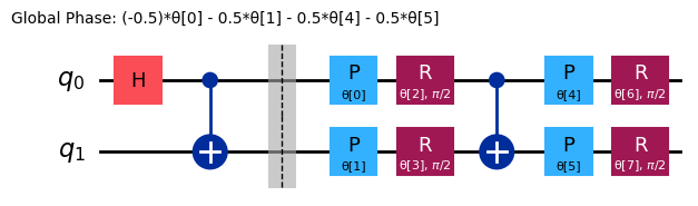
สำหรับ Circuit ใหม่นี้ solution ที่ ideal จะได้เมื่อ parameter ทั้งหมดเป็น $0$ ซึ่งยืนยันว่าการเลือก reference circuit นั้นสมเหตุสมผล

ตอนนี้เราเปรียบเทียบจำนวนการประเมิน cost function จำนวน iteration ของ optimizer และเวลาที่ใช้กับความพยายามก่อนหน้า

import time

start_time = time.time()

ref_result = minimize(
    cost_func_vqe, x0, args=(ref_ansatz, observable_1, estimator), method="COBYLA"
)

end_time = time.time()
execution_time = end_time - start_time

ใช้ parameter ที่ optimal เพื่อคำนวณค่า eigenvalue ต่ำสุด:

experimental_min_eigenvalue_ref = cost_func_vqe(
    ref_result.x, ref_ansatz, observable_1, estimator
)
print(experimental_min_eigenvalue_ref)

-5.999999996759607

print("ADDED REFERENCE STATE:")
print(f"""Number of iterations: {ref_result.nfev}""")
print(f"""Time (s): {execution_time}""")
print(
    f"Percent error: {100*abs((experimental_min_eigenvalue_ref - solution_eigenvalue)/solution_eigenvalue):.2e}"
)

ADDED REFERENCE STATE:
Number of iterations: 127
Time (s): 0.5620882511138916
Percent error: 5.40e-08

ขึ้นอยู่กับระบบของคุณ อาจจะเร็วขึ้นหรือแม่นยำขึ้นหรือไม่ก็ได้ในตัวอย่างขนาดเล็กมากนี้ ประเด็นสำคัญคือ การเริ่มต้นด้วย reference state ที่อิงจากฟิสิกส์จะยิ่งสำคัญขึ้นเรื่อย ๆ ในการเพิ่มความเร็วและความแม่นยำเมื่อปัญหามีขนาดใหญ่ขึ้น

เปลี่ยน initial point

เมื่อเห็นผลของการเพิ่ม reference state แล้ว เราจะสำรวจผลที่เกิดขึ้นเมื่อเลือก initial point $\vec{\theta_0}$ ต่างกัน โดยเฉพาะอย่างยิ่งเราจะใช้ $\vec{\theta_0}=(0,0,0,0,6,0,0,0)$ และ $\vec{\theta_0}=(6,6,6,6,6,6,6,6,6)$

จำไว้ว่า ตามที่กล่าวถึงตอนแนะนำ reference state solution ที่ ideal จะพบเมื่อ parameter ทั้งหมดเป็น $0$ ดังนั้น initial point แรกควรใช้จำนวน evaluation น้อยกว่า

import time

start_time = time.time()

x0 = [0, 0, 0, 0, 6, 0, 0, 0]

x0_1_result = minimize(
    cost_func_vqe, x0, args=(raw_ansatz, observable_1, estimator), method="COBYLA"
)

end_time = time.time()
execution_time = end_time - start_time

print("INITIAL POINT 1:")
print(f"""Number of iterations: {x0_1_result.nfev}""")
print(f"""Time (s): {execution_time}""")

INITIAL POINT 1:
Number of iterations: 108
Time (s): 0.4492197036743164

ปรับ initial point เป็น $\vec{\theta_0}=(6,6,6,6,6,6,6,6,6)$:

import time

start_time = time.time()

x0 = 6 * np.ones(raw_ansatz.num_parameters)

x0_2_result = minimize(
    cost_func_vqe, x0, args=(raw_ansatz, observable_1, estimator), method="COBYLA"
)

end_time = time.time()
execution_time = end_time - start_time

print("INITIAL POINT 2:")
print(f"""Number of iterations: {x0_2_result.nfev}""")
print(f"""Time (s): {execution_time}""")

INITIAL POINT 2:
Number of iterations: 107
Time (s): 0.40889453887939453

การทดลองกับ initial point ต่าง ๆ อาจช่วยให้ convergence เร็วขึ้นและใช้จำนวน function evaluation น้อยลง

ทดลองกับ optimizer ต่าง ๆ

เราสามารถปรับ optimizer โดยใช้ argument method ของ SciPy minimize โดยดูตัวเลือกเพิ่มเติมได้ที่นี่ เดิมเราใช้ constrained minimizer (COBYLA) ในตัวอย่างนี้ เราจะลองใช้ unconstrained minimizer (BFGS) แทน

import time

start_time = time.time()

result = minimize(
    cost_func_vqe, x0, args=(raw_ansatz, observable_1, estimator), method="BFGS"
)

end_time = time.time()
execution_time = end_time - start_time

print("CHANGED TO BFGS OPTIMIZER:")
print(f"""Number of iterations: {result.nfev}""")
print(f"""Time (s): {execution_time}""")

CHANGED TO BFGS OPTIMIZER:
Number of iterations: 117
Time (s): 0.31656408309936523

ตัวอย่าง VQD

ที่นี่เราจะ implement Qiskit patterns framework อย่างชัดเจน

ขั้นตอนที่ 1: แมป input แบบ classical ไปสู่ปัญหา quantum

แทนที่จะหาแค่ค่า eigenvalue ต่ำสุดของ observable เราจะหาทั้ง $4$ ค่า (โดย $k=4$)

จำไว้ว่า cost function ของ VQD คือ:

$$C_{l}(\vec{\theta}) := \langle \psi(\vec{\theta}) | \hat{H} | \psi(\vec{\theta})\rangle + \sum_{j=0}^{l-1}\beta_j |\langle \psi(\vec{\theta})| \psi(\vec{\theta^j})\rangle |^2 \quad \forall l\in\{1,\cdots,k\}=\{1,\cdots,4\}$$

สิ่งนี้สำคัญมากเพราะต้องส่ง vector $\vec{\beta}=(\beta_0,\cdots,\beta_{k-1})$ (ในกรณีนี้คือ $(\beta_0, \beta_1, \beta_2, \beta_3)$) เป็น argument เมื่อนิยาม object VQD

นอกจากนี้ ใน Qiskit's implementation ของ VQD แทนที่จะพิจารณา effective observable ที่อธิบายใน notebook ก่อนหน้า ค่า fidelity $|\langle \psi(\vec{\theta})| \psi(\vec{\theta^j})\rangle |^2$ จะคำนวณโดยตรงผ่านอัลกอริทึม ComputeUncompute ซึ่งใช้ Sampler primitive เพื่อ sample ความน่าจะเป็นของการได้ $|0\rangle$ จาก Circuit $U_A^\dagger(\vec{\theta})U_A(\vec{\theta^j})$ ซึ่งทำงานได้เพราะความน่าจะเป็นนี้คือ

$$\begin{aligned} p_0 & = |\langle 0|U_A^\dagger(\vec{\theta})U_A(\vec{\theta^j})|0\rangle|^2 \\[1mm] & = |\big(\langle 0|U_A^\dagger(\vec{\theta})\big)\big(U_A(\vec{\theta^j})|0\rangle\big)|^2 \\[1mm] & = |\langle \psi(\vec{\theta}) |\psi(\vec{\theta^j}) \rangle|^2 \\[1mm] \end{aligned}$$

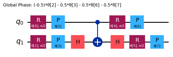
ansatz = n_local(
    num_qubits=2,
    rotation_blocks=["ry", "rz"],
    entanglement_blocks="cz",
    #    entanglement="linear",
    reps=1,
)

ansatz.decompose().draw("mpl")

เริ่มต้นด้วยการตรวจสอบ observable ต่อไปนี้:

$$\hat{O}_2 := 2 II - 3 XX + 2 YY - 4 ZZ$$

observable นี้มีค่า eigenvalue ดังนี้:

$$\left\{ \begin{array}{c} \lambda_0 = -7 \\ \lambda_1 = 3\\ \lambda_2 = 5 \\ \lambda_3 = 7 \end{array} \right\}$$

และ eigenstate:

$$\left\{ \begin{array}{c} |\phi_0\rangle = \frac{1}{\sqrt{2}}(|00\rangle + |11\rangle)\\ |\phi_1\rangle = \frac{1}{\sqrt{2}}(|00\rangle - |11\rangle)\\ |\phi_2\rangle = \frac{1}{\sqrt{2}}(|01\rangle + |10\rangle)\\ |\phi_3\rangle = \frac{1}{\sqrt{2}}(|01\rangle - |10\rangle) \end{array} \right\}$$

from qiskit.quantum_info import SparsePauliOp

observable_2 = SparsePauliOp.from_list([("II", 2), ("XX", -3), ("YY", 2), ("ZZ", -4)])

เราจะใช้ฟังก์ชันต่อไปนี้เพื่อคำนวณ overlap penalty สังเกตว่านี่ยังเป็นส่วนหนึ่งของการแมปปัญหาไปสู่ quantum circuit อย่างไรก็ตาม ตามที่กล่าวถึงใน lesson ก่อนหน้า ฟังก์ชันนี้คำนวณ overlap ระหว่าง variational circuit ปัจจุบันกับ circuit ที่ optimize แล้วจาก state ที่มีพลังงาน/ต้นทุนต่ำกว่าซึ่งได้มาก่อนหน้า Circuit ใหม่ที่สร้างขึ้นยังต้อง transpile เพื่อรันบน hardware จริงด้วย เราเคยเห็นฟังก์ชันนี้มาก่อนบน simulator ที่นี่เราต้องพิจารณา transpile และการ optimize ที่เกี่ยวข้องสำหรับ real backend ไว้ล่วงหน้า ดังนั้นจึงมีบรรทัดเกี่ยวกับ if realbackend == 1 ซึ่งเป็นการผสมขั้นตอนที่ 2 เข้ามาบ้าง แต่เราจะระบุขั้นตอนที่ 2 อย่างชัดเจนในภายหลัง

import numpy as np
from qiskit.transpiler.preset_passmanagers import generate_preset_pass_manager

def calculate_overlaps(
    ansatz, prev_circuits, parameters, sampler, realbackend, backend
):
    def create_fidelity_circuit(circuit_1, circuit_2):
        if len(circuit_1.clbits) > 0:
            circuit_1.remove_final_measurements()
        if len(circuit_2.clbits) > 0:
            circuit_2.remove_final_measurements()

        circuit = circuit_1.compose(circuit_2.inverse())
        circuit.measure_all()
        return circuit

    overlaps = []

    for prev_circuit in prev_circuits:
        fidelity_circuit = create_fidelity_circuit(ansatz, prev_circuit)
        if realbackend == 1:
            pm = generate_preset_pass_manager(backend=backend, optimization_level=3)
            fidelity_circuit = pm.run(fidelity_circuit)
        sampler_job = sampler.run([(fidelity_circuit, parameters)])
        meas_data = sampler_job.result()[0].data.meas

        counts_0 = meas_data.get_int_counts().get(0, 0)
        shots = meas_data.num_shots
        overlap = counts_0 / shots
        overlaps.append(overlap)

    return np.array(overlaps)

ตอนนี้เราเพิ่ม cost function ของ VQD สังเกตว่าเมื่อเทียบกับ lesson ก่อนหน้า เรามี argument เพิ่มสองตัว (realbackend และ backend) เพื่อช่วย transpile เมื่อใช้ real backend

def cost_func_vqd(
    parameters,
    ansatz,
    prev_states,
    step,
    betas,
    estimator,
    sampler,
    hamiltonian,
    realbackend,
    backend,
):
    estimator_job = estimator.run([(ansatz, hamiltonian, [parameters])])

    total_cost = 0

    if step > 1:
        overlaps = calculate_overlaps(
            ansatz, prev_states, parameters, sampler, realbackend, backend
        )
        total_cost = np.sum(
            [np.real(betas[state] * overlap) for state, overlap in enumerate(overlaps)]
        )

    estimator_result = estimator_job.result()[0]

    value = estimator_result.data.evs[0] + total_cost

    return value

เราจะใช้ simulator ในการ debug ก่อน แล้วจึงเปลี่ยนไปใช้ hardware จริง

from qiskit.primitives import StatevectorSampler
from qiskit.primitives import StatevectorEstimator

sampler = StatevectorSampler(default_shots=4092)
estimator = StatevectorEstimator()

ที่นี่เราระบุจำนวน state ที่ต้องการคำนวณ ค่า penalty และชุด parameter เริ่มต้น x0

from qiskit.quantum_info import SparsePauliOp

k = 4
betas = [50, 60, 40]
x0 = np.ones(8)

เราจะทดสอบอัลกอริทึมโดยใช้ simulator:

from scipy.optimize import minimize

prev_states = []
prev_opt_parameters = []
eigenvalues = []

realbackend = 0

for step in range(1, k + 1):
    if step > 1:
        prev_states.append(ansatz.assign_parameters(prev_opt_parameters))

    result = minimize(
        cost_func_vqd,
        x0,
        args=(
            ansatz,
            prev_states,
            step,
            betas,
            estimator,
            sampler,
            observable_2,
            realbackend,
            None,
        ),
        method="COBYLA",
        options={"maxiter": 200, "tol": 0.000001},
    )
    print(result)

    prev_opt_parameters = result.x
    eigenvalues.append(result.fun)

message: Return from COBYLA because the trust region radius reaches its lower bound.
 success: True
  status: 0
     fun: -6.9999999999996
       x: [ 1.571e+00  1.571e+00  2.519e+00  2.100e+00  1.242e+00
            6.935e-01  2.298e+00  1.991e+00]
    nfev: 151
   maxcv: 0.0
 message: Return from COBYLA because the trust region radius reaches its lower bound.
 success: True
  status: 0
     fun: 3.698974255258432
       x: [ 1.269e+00  1.109e+00  1.080e+00  1.200e+00  1.094e+00
            1.163e+00  9.752e-01  9.519e-01]
    nfev: 103
   maxcv: 0.0
 message: Return from COBYLA because the trust region radius reaches its lower bound.
 success: True
  status: 0
     fun: 4.731320121938101
       x: [ 1.533e+00  2.451e+00  2.526e+00  2.406e+00  1.968e+00
            2.105e+00  8.537e-01  8.442e-01]
    nfev: 110
   maxcv: 0.0
 message: Return from COBYLA because the trust region radius reaches its lower bound.
 success: True
  status: 0
     fun: 7.008239313655201
       x: [ 4.150e+00  2.120e+00  3.495e+00  7.262e-01  1.953e+00
           -1.982e-01  3.263e-01  2.563e+00]
    nfev: 126
   maxcv: 0.0

eigenvalues

[np.float64(-6.9999999999996),
 np.float64(3.698974255258432),
 np.float64(4.731320121938101),
 np.float64(7.008239313655201)]

ผลลัพธ์เหล่านี้ใกล้เคียงกับค่าที่คาดหวังพอสมควร ยกเว้น approximation error และ global phase เราสามารถปรับ tolerance ของ classical optimizer และ/หรือค่า penalty สำหรับ statevector overlap เพื่อให้ได้ค่าที่แม่นยำยิ่งขึ้น

solution_eigenvalues = [-7, 3, 5, 7]

for index, experimental_eigenvalue in enumerate(eigenvalues):
    solution_eigenvalue = solution_eigenvalues[index]

    print(
        f"Percent error: {abs((experimental_eigenvalue - solution_eigenvalue)/solution_eigenvalue):.2e}"
    )

Percent error: 5.71e-14
Percent error: 2.33e-01
Percent error: 5.37e-02
Percent error: 1.18e-03

เปลี่ยนค่า betas

ตามที่กล่าวถึงใน lesson ก่อนหน้า ค่า $\vec{\beta}$ ควรมากกว่าความแตกต่างระหว่าง eigenvalue ลองดูว่าจะเกิดอะไรขึ้นเมื่อไม่เป็นไปตามเงื่อนไขนั้นกับ $\hat{O}_2$

$$\hat{O}_2 = 2 II - 3 XX + 2 YY - 4 ZZ$$

ซึ่งมีค่า eigenvalue

$$\left\{ \begin{array}{c} \lambda_0 = -7 \\ \lambda_1 = 3\\ \lambda_2 = 5 \\ \lambda_3 = 7 \end{array} \right\}$$

from qiskit.quantum_info import SparsePauliOp

k = 4
betas = np.ones(3)
x0 = np.zeros(8)

from scipy.optimize import minimize

prev_states = []
prev_opt_parameters = []
eigenvalues = []

realbackend = 0

for step in range(1, k + 1):
    if step > 1:
        prev_states.append(ansatz.assign_parameters(prev_opt_parameters))

    result = minimize(
        cost_func_vqd,
        x0,
        args=(
            ansatz,
            prev_states,
            step,
            betas,
            estimator,
            sampler,
            observable_2,
            realbackend,
            None,
        ),
        method="COBYLA",
        options={"tol": 0.01, "maxiter": 200},
    )
    print(result)

    prev_opt_parameters = result.x
    eigenvalues.append(result.fun)

message: Return from COBYLA because the trust region radius reaches its lower bound.
 success: True
  status: 0
     fun: -6.999916534745094
       x: [ 1.568e+00 -1.569e+00  1.385e-01  1.398e-01 -7.972e-01
            7.835e-01 -2.375e-01  4.539e-02]
    nfev: 125
   maxcv: 0.0
 message: Return from COBYLA because the trust region radius reaches its lower bound.
 success: True
  status: 0
     fun: -1.515139929812874
       x: [-5.317e-04 -2.514e-03  1.016e+00  9.998e-01  3.890e-04
            1.772e-04  1.568e-04  8.497e-04]
    nfev: 35
   maxcv: 0.0
 message: Return from COBYLA because the trust region radius reaches its lower bound.
 success: True
  status: 0
     fun: -0.509948114293115
       x: [-3.796e-03  8.853e-03  3.015e-04  9.997e-01  6.271e-04
           -2.554e-03  1.017e-04  2.766e-04]
    nfev: 37
   maxcv: 0.0
 message: Return from COBYLA because the trust region radius reaches its lower bound.
 success: True
  status: 0
     fun: 0.4914672235935682
       x: [-7.178e-03 -8.652e-03  1.125e+00 -5.428e-02 -1.586e-03
            2.031e-03 -3.462e-03  5.734e-03]
    nfev: 35
   maxcv: 0.0

solution_eigenvalues = [-7, 3, 5, 7]

for index, experimental_eigenvalue in enumerate(eigenvalues):
    solution_eigenvalue = solution_eigenvalues[index]

    print(
        f"Percent error: {abs((experimental_eigenvalue - solution_eigenvalue)/solution_eigenvalue):.2e}"
    )

Percent error: 1.19e-05
Percent error: 1.51e+00
Percent error: 1.10e+00
Percent error: 9.30e-01

คราวนี้ optimizer ส่งคืน state $|\phi_0\rangle = \frac{1}{\sqrt{2}}(|00\rangle + |11\rangle)$ เดิมเป็น solution ที่เสนอสำหรับ eigenstate ทุกตัว ซึ่งผิดอย่างชัดเจน เหตุการณ์นี้เกิดขึ้นเพราะ betas เล็กเกินไปจนไม่สามารถ penalize minimum eigenstate ใน cost function รอบต่อ ๆ มาได้ จึงไม่ถูกกำจัดออกจาก search space ที่ใช้งานได้ในการ iterate ครั้งต่อมา และถูกเลือกเป็น solution ที่ดีที่สุดเสมอ

เราแนะนำให้ทดลองกับค่า $\vec{\beta}$ และมั่นใจว่ามันมากกว่าความแตกต่างระหว่าง eigenvalue

ขั้นตอนที่ 2: Optimize ปัญหาสำหรับการประมวลผล quantum

เพื่อรันบน hardware จริง เราต้อง optimize quantum circuit สำหรับ quantum computer ที่เลือก ในที่นี้เราจะใช้ backend ที่ว่างน้อยที่สุด

from qiskit_ibm_runtime import SamplerV2 as Sampler
from qiskit_ibm_runtime import EstimatorV2 as Estimator
from qiskit_ibm_runtime import Session, EstimatorOptions
from qiskit_ibm_runtime import QiskitRuntimeService

service = QiskitRuntimeService()
backend = service.least_busy(operational=True, simulator=False)
# Or use a specific backend
# backend = service.backend("ibm_brisbane")
print(backend)

<IBMBackend('ibm_brisbane')>

เราจะ transpile Circuit โดยใช้ preset pass manager และ optimization level 3

pm = generate_preset_pass_manager(backend=backend, optimization_level=3)
isa_ansatz = pm.run(ansatz)
isa_observable = observable_2.apply_layout(layout=isa_ansatz.layout)

ขั้นตอนที่ 3: Execute โดยใช้ Qiskit primitives

โดยดูแลให้ reset betas กลับเป็นค่าสูงพอ เราสามารถรันการคำนวณบน real quantum hardware ได้

# Estimated compute resource usage: 25 minutes. Benchmarked at 24 min, 30 sec on an Eagle r3 processor on 5-30-24

k = 2
betas = [30, 50, 80]
x0 = np.zeros(8)

real_prev_states = []
real_prev_opt_parameters = []
real_eigenvalues = []

realbackend = 1

estimator_options = EstimatorOptions(resilience_level=1, default_shots=10_000)

with Session(backend=backend) as session:
    estimator = Estimator(mode=session, options=estimator_options)
    sampler = Sampler(mode=session)

    for step in range(1, k + 1):
        if step > 1:
            real_prev_states.append(isa_ansatz.assign_parameters(prev_opt_parameters))

        result = minimize(
            cost_func_vqd,
            x0,
            args=(
                isa_ansatz,
                real_prev_states,
                step,
                betas,
                estimator,
                sampler,
                isa_observable,
                realbackend,
                backend,
            ),
            method="COBYLA",
            options={"maxiter": 200},
        )
        print(result)

        real_prev_opt_parameters = result.x
        real_eigenvalues.append(result.fun)

session.close()
print(real_eigenvalues)

ขั้นตอนที่ 4: Post-process คืนผลในรูปแบบ classical

output ของเรามีโครงสร้างคล้ายกับที่กล่าวถึงใน lesson และตัวอย่างก่อนหน้า แต่มีบางอย่างที่มีปัญหาในผลลัพธ์ข้างต้น ซึ่งเราสามารถสรุปเป็นข้อเตือนใจสำหรับบริบทของ excited state เพื่อจำกัดเวลาประมวลผลที่ใช้ใน learning example นี้ เราตั้งจำนวน iteration สูงสุดสำหรับ classical optimizer ไว้ที่ 200 ซึ่งอาจต่ำเกินไป: การคำนวณก่อนหน้าบน simulator ไม่ converge ใน 200 iteration ที่นี่ converge แล้ว... แต่ด้วย tolerance เท่าไร เราไม่ได้ระบุ tolerance ให้ COBYLA เพื่อพิจารณาว่า "converge" แล้ว การดูที่ค่า function และเปรียบเทียบกับการรันก่อนหน้าบอกเราว่า COBYLA ยังไม่ใกล้ converge ถึง precision ที่ต้องการ

มีปัญหาอีกประการ: พลังงานของ first excited state ดูเหมือนต่ำกว่าพลังงาน ground state! ลองอธิบายว่าเหตุการณ์นี้เกิดขึ้นได้อย่างไร คำใบ้: เกี่ยวข้องกับ convergence point ที่เราเพิ่งกล่าวถึง พฤติกรรมนี้อธิบายอย่างละเอียดด้านล่างหลังจากนำ VQD ไปใช้กับโมเลกุล H2

เคมีควอนตัม: ตัวแก้พลังงาน ground state และ excited state

เป้าหมายของเราคือ minimize ค่าคาดหวังของ observable ที่แทนพลังงาน (Hamiltonian $\hat{\mathcal{H}}$):

$$\min_{\vec\theta} \langle\psi(\vec\theta)|\hat{\mathcal{H}}|\psi(\vec\theta)\rangle$$

from qiskit.quantum_info import SparsePauliOp
from qiskit.circuit.library import efficient_su2

H2_op = SparsePauliOp.from_list(
    [
        ("II", -1.052373245772859),
        ("IZ", 0.39793742484318045),
        ("ZI", -0.39793742484318045),
        ("ZZ", -0.01128010425623538),
        ("XX", 0.18093119978423156),
    ]
)

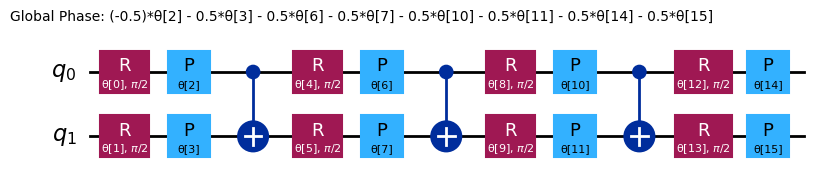
chem_ansatz = efficient_su2(H2_op.num_qubits)

chem_ansatz.decompose().draw("mpl")

from qiskit import QuantumCircuit

def cost_func_vqe(params, ansatz, hamiltonian, estimator):
    """Return estimate of energy from estimator

    Parameters:
        params (ndarray): Array of ansatz parameters
        ansatz (QuantumCircuit): Parameterized ansatz circuit
        hamiltonian (SparsePauliOp): Operator representation of Hamiltonian
        estimator (Estimator): Estimator primitive instance

    Returns:
        float: Energy estimate
    """
    pub = (ansatz, hamiltonian, params)
    cost = estimator.run([pub]).result()[0].data.evs
    #    cost = estimator.run(ansatz, hamiltonian, parameter_values=params).result().values[0]
    return cost

เราตั้งค่า parameter เริ่มต้น:

import numpy as np

x0 = np.ones(chem_ansatz.num_parameters)

เราสามารถ minimize cost function นี้เพื่อคำนวณ parameter ที่เหมาะสมที่สุด และตรวจสอบโค้ดของเราก่อนโดยใช้ local simulator

from qiskit.primitives import StatevectorEstimator as Estimator
from qiskit.primitives import StatevectorSampler as Sampler

estimator = Estimator()
sampler = Sampler()

# SciPy minimizer routine
from scipy.optimize import minimize
import time

start_time = time.time()

result = minimize(
    cost_func_vqe, x0, args=(chem_ansatz, H2_op, estimator), method="COBYLA"
)

end_time = time.time()
execution_time = end_time - start_time

result

message: Optimization terminated successfully.
 success: True
  status: 1
     fun: -1.857275029048451
       x: [ 7.326e-01  1.354e+00 ...  1.040e+00  1.508e+00]
    nfev: 242
   maxcv: 0.0

ค่าต่ำสุดของ cost function (-1.857...) คือพลังงาน ground state ของโมเลกุล H2 ในหน่วย hartrees

Excited States

เราสามารถใช้ VQD เพื่อแก้หา $k=2$ state ทั้งหมด (ground state และ first excited state)

from qiskit.quantum_info import SparsePauliOp
import numpy as np

k = 2
betas = [33, 33]
# x0 = np.zeros(ansatz.num_parameters)
x0 = [
    1.164e00,
    -2.438e-01,
    9.358e-04,
    6.745e-02,
    1.990e00,
    9.810e-02,
    6.154e-01,
    5.454e-01,
]

เราจะเพิ่มการคำนวณ overlap:

from scipy.optimize import minimize

prev_states = []
prev_opt_parameters = []
eigenvalues = []

realbackend = 0

for step in range(1, k + 1):
    if step > 1:
        prev_states.append(ansatz.assign_parameters(prev_opt_parameters))

    result = minimize(
        cost_func_vqd,
        x0,
        args=(
            ansatz,
            prev_states,
            step,
            betas,
            estimator,
            sampler,
            H2_op,
            realbackend,
            None,
        ),
        method="COBYLA",
        options={"tol": 0.001, "maxiter": 2000},
    )
    print(result)

    prev_opt_parameters = result.x
    eigenvalues.append(result.fun)

message: Optimization terminated successfully.
 success: True
  status: 1
     fun: -1.8572671093941977
       x: [ 1.164e+00 -2.437e-01  2.118e-03  6.448e-02  1.990e+00
            9.870e-02  6.167e-01  5.476e-01]
    nfev: 58
   maxcv: 0.0
 message: Optimization terminated successfully.
 success: True
  status: 1
     fun: -1.0322873777662176
       x: [ 3.205e+00  1.502e+00  1.699e+00 -1.107e-02  3.086e+00
            1.530e+00  4.445e-02  7.013e-02]
    nfev: 99
   maxcv: 0.0

eigenvalues

[-1.8572671093941977, -1.0322873777662176]

Hardware จริงและข้อเตือนใจสุดท้าย

เพื่อรันบน hardware จริง เราต้อง optimize quantum circuit สำหรับ quantum computer ที่เลือก ในที่นี้เราจะใช้ backend ที่ว่างน้อยที่สุด

from qiskit_ibm_runtime import SamplerV2 as Sampler
from qiskit_ibm_runtime import EstimatorV2 as Estimator
from qiskit_ibm_runtime import Session, EstimatorOptions
from qiskit_ibm_runtime import QiskitRuntimeService

service = QiskitRuntimeService()
backend = service.least_busy(operational=True, simulator=False)

เราจะใช้ preset pass manager สำหรับ transpilation และ optimize Circuit อย่างสูงสุดด้วย optimization level 3

from qiskit.transpiler.preset_passmanagers import generate_preset_pass_manager

pm = generate_preset_pass_manager(backend=backend, optimization_level=3)
isa_ansatz = pm.run(ansatz)
isa_observable = H2_op.apply_layout(layout=isa_ansatz.layout)

เนื่องจาก VQD มีการ iterate สูงมาก เราจะดำเนินการทุกขั้นตอนภายใน Runtime Session เพื่อให้ job ถูกคิวครั้งเดียวตอนต้น ไม่ใช่ระหว่างการอัปเดต parameter ทุกครั้ง ไม่มีอะไรเปลี่ยนแปลงใน syntax ของ cost function หรือ Estimator

x0 = [
    1.306e00,
    -2.284e-01,
    6.913e-02,
    -2.530e-02,
    1.849e00,
    7.433e-02,
    6.366e-01,
    5.600e-01,
]

# Estimated hardware usage: 20 min benchmarked on an Eagle r3 processor on 5-30-24

real_prev_states = []
real_prev_opt_parameters = []
real_eigenvalues = []

realbackend = 1

estimator_options = EstimatorOptions(resilience_level=1, default_shots=4096)

with Session(backend=backend) as session:
    estimator = Estimator(mode=session)
    sampler = Sampler(mode=session)

    for step in range(1, k + 1):
        if step > 1:
            real_prev_states.append(
                isa_ansatz.assign_parameters(real_prev_opt_parameters)
            )

        result = minimize(
            cost_func_vqd,
            x0,
            args=(
                isa_ansatz,
                real_prev_states,
                step,
                betas,
                estimator,
                sampler,
                isa_observable,
                realbackend,
                backend,
            ),
            method="COBYLA",
            options={"tol": 0.001, "maxiter": 300},
        )
        print(result)

        real_prev_opt_parameters = result.x
        real_eigenvalues.append(result.fun)

session.close()
print(real_eigenvalues)

พลังงาน ground state ที่ได้ (-1.83 hartrees) ไม่ต่างจากค่าที่ถูกต้องมากนัก (-1.85 hartrees) อย่างไรก็ตาม พลังงาน excited state ผิดพลาดค่อนข้างมาก ซึ่งคล้ายกับพฤติกรรมผิดปกติที่เราเห็นก่อนหน้าในบทเรียนนี้ พลังงานที่รายงานสำหรับ excited state ใกล้เคียงกับ ground state มาก ในกรณีก่อนหน้านั้น เราเห็น excited state energy ที่ ต่ำกว่า ground state energy ที่รายงานด้วยซ้ำ

การคำนวณแบบ variational ไม่สามารถให้พลังงานที่ต่ำกว่า ground state energy จริง ๆ ได้ ในกรณีก่อนหน้านั้น ground state energy ที่เราได้ไม่ใกล้เคียงกับ ground state จริง เนื่องจากเราไม่ได้ค่า ground state energy จริงในกรณีนั้น จึงไม่มีความขัดแย้ง ในกรณีปัจจุบัน ground state energy ใกล้เคียงค่าที่ถูกต้องพอสมควร แต่ excited state energy ดูเหมือนใกล้เคียงกับค่าเดียวกันอย่างแปลก ๆ

เพื่อทำความเข้าใจว่าเกิดอะไรขึ้น จำไว้ว่าวิธีที่เราหา excited state คือการบังคับให้ variational state ตั้งฉากกับ ground state (โดยใช้ overlap circuit และ penalty term) หากเราไม่สามารถหาพลังงาน ground state ที่แม่นยำได้ (หรือผิดพลาดสักเปอร์เซ็นต์) เราก็ไม่สามารถหา ground state vector ที่แม่นยำได้เช่นกัน ดังนั้นเมื่อเราบังคับให้ excited state ตั้งฉากกับ state แรกที่หาได้ เรากำลัง impose orthogonality กับ approximation ของ ground state (บางครั้ง approximation ที่ไม่ค่อยดี) ไม่ใช่กับ ground state จริง ดังนั้น excited state จึงไม่ถูกบังคับให้ตั้งฉากกับ ground state จริง และการประมาณพลังงานสำหรับ excited state จึงใกล้เคียงกับ ground state energy มาก

ปัญหานี้จะเป็นข้อกังวลเสมอใน VQD แต่โดยหลักการแล้ว สามารถแก้ไขได้โดยเพิ่มจำนวน iteration สูงสุดสำหรับ classical optimizer กำหนด tolerance ที่ต่ำกว่าสำหรับ classical optimizer และอาจลองใช้ ansatz อื่นหากเราพลาด ground state จริงซ้ำ ๆ เราอาจต้องปรับ overlap penalty (betas) ด้วย แต่นั่นเป็นประเด็นแยกต่างหาก ไม่มี penalty สำหรับ overlap ใดที่จะทำให้คุณห่างจาก ground state จริง ถ้าคุณยังไม่ได้ estimation ที่ดีมากพอสำหรับ true ground state ใน overlap circuit

การ Optimization: Max-Cut

ปัญหา maximum cut (Max-Cut) เป็นปัญหา combinatorial optimization ที่เกี่ยวกับการแบ่ง vertex ของกราฟออกเป็นสองกลุ่มที่ disjoint เพื่อให้จำนวน edge ระหว่างสองกลุ่มมีค่าสูงสุด อย่างเป็นทางการ กำหนดกราฟไม่มีทิศทาง $G=(V,E)$ ซึ่ง $V$ คือเซตของ vertex และ $E$ คือเซตของ edge ปัญหา Max-Cut คือการแบ่ง vertex ออกเป็นสองกลุ่ม $S$ และ $T$ ที่ disjoint เพื่อให้จำนวน edge ที่มี endpoint อยู่ใน $S$ และอีกปลายใน $T$ มีค่าสูงสุด

เราสามารถนำ Max-Cut ไปใช้แก้ปัญหาต่าง ๆ เช่น clustering, network design และ phase transition เริ่มต้นด้วยการสร้างกราฟปัญหา:

import rustworkx as rx
from rustworkx.visualization import mpl_draw

n = 4
G = rx.PyGraph()
G.add_nodes_from(range(n))
# The edge syntax is (start, end, weight)
edges = [(0, 1, 1.0), (0, 2, 1.0), (0, 3, 1.0), (1, 2, 1.0), (2, 3, 1.0)]
G.add_edges_from(edges)

mpl_draw(
    G, pos=rx.shell_layout(G), with_labels=True, edge_labels=str, node_color="#1192E8"
)

ปัญหานี้สามารถแสดงเป็น binary optimization problem สำหรับ node แต่ละตัว $0 \leq i < n$ ซึ่ง $n$ คือจำนวน node ของกราฟ (ในกรณีนี้ $n=4$) เราจะใช้ตัวแปร binary $x_i$ ตัวแปรนี้มีค่า $1$ ถ้า node $i$ อยู่ในกลุ่มที่เราจะเรียกว่า $1$ และ $0$ ถ้าอยู่ในกลุ่มอื่นที่เรียกว่า $0$ เราจะแทน $w_{ij}$ (element $(i,j)$ ของ adjacency matrix $w$) เป็นน้ำหนักของ edge ที่ไปจาก node $i$ ถึง node $j$ เนื่องจากกราฟไม่มีทิศทาง $w_{ij}=w_{ji}$ เราสามารถกำหนดปัญหาเป็นการ maximize cost function ต่อไปนี้:

$$\begin{aligned} C(\vec{x}) & =\sum_{i,j=0}^n w_{ij} x_i(1-x_j)\\[1mm] & = \sum_{i,j=0}^n w_{ij} x_i - \sum_{i,j=0}^n w_{ij} x_ix_j\\[1mm] & = \sum_{i,j=0}^n w_{ij} x_i - \sum_{i=0}^n \sum_{j=0}^i 2w_{ij} x_ix_j \end{aligned}$$

เพื่อแก้ปัญหานี้ด้วยคอมพิวเตอร์ quantum เราจะแสดง cost function เป็นค่าคาดหวังของ observable อย่างไรก็ตาม observable ที่ Qiskit รองรับแบบ native ประกอบด้วย Pauli operator ที่มีค่า eigenvalue $1$ และ $-1$ แทนที่จะเป็น $0$ และ $1$ นั่นคือเหตุผลที่เราจะทำการเปลี่ยนตัวแปรดังนี้:

โดยที่ $\vec{x}=(x_0,x_1,\cdots ,x_{n-1})$ เราสามารถใช้ adjacency matrix $w$ เพื่อเข้าถึงน้ำหนักของ edge ทั้งหมดได้อย่างสะดวก ซึ่งจะนำไปสู่ cost function:

$$z_i = 1-2x_i \rightarrow x_i = \frac{1-z_i}{2}$$

ซึ่งหมายความว่า:

$$\begin{array}{lcl} x_i=0 & \rightarrow & z_i=1 \\ x_i=1 & \rightarrow & z_i=-1.\end{array}$$

ดังนั้น cost function ใหม่ที่เราต้องการ maximize คือ:

$$\begin{aligned} C(\vec{z}) & = \sum_{i,j=0}^n w_{ij} \bigg(\frac{1-z_i}{2}\bigg)\bigg(1-\frac{1-z_j}{2}\bigg)\\[1mm] & = \sum_{i,j=0}^n \frac{w_{ij}}{4} - \sum_{i,j=0}^n \frac{w_{ij}}{4} z_iz_j\\[1mm] & = \sum_{i=0}^n \sum_{j=0}^i \frac{w_{ij}}{2} - \sum_{i=0}^n \sum_{j=0}^i \frac{w_{ij}}{2} z_iz_j \end{aligned}$$

นอกจากนี้ คอมพิวเตอร์ quantum มีแนวโน้มตามธรรมชาติที่จะหาค่าต่ำสุด (โดยทั่วไปคือพลังงานต่ำสุด) แทนที่จะเป็นค่าสูงสุด ดังนั้นแทนที่จะ maximize $C(\vec{z})$ เราจะ minimize:

$$-C(\vec{z}) = \sum_{i=0}^n \sum_{j=0}^i \frac{w_{ij}}{2} z_iz_j - \sum_{i=0}^n \sum_{j=0}^i \frac{w_{ij}}{2}$$

เมื่อเรามี cost function ที่ต้อง minimize ซึ่งตัวแปรมีค่า $-1$ และ $1$ ได้ เราสามารถทำ analogy กับ Pauli $Z$ ดังนี้:

$$z_i \equiv Z_i = \overbrace{I}^{n-1}\otimes ... \otimes \overbrace{Z}^{i} \otimes ... \otimes \overbrace{I}^{0}$$

กล่าวอีกนัยหนึ่ง ตัวแปร $z_i$ จะเทียบเท่ากับ $Z$ Gate ที่กระทำบน Qubit $i$ นอกจากนี้:

$$Z_i|x_{n-1}\cdots x_0\rangle = z_i|x_{n-1}\cdots x_0\rangle \rightarrow \langle x_{n-1}\cdots x_0 |Z_i|x_{n-1}\cdots x_0\rangle = z_i$$

ดังนั้น observable ที่เราจะพิจารณาคือ:

$$\hat{H} = \sum_{i=0}^n \sum_{j=0}^i \frac{w_{ij}}{2} Z_iZ_j$$

ซึ่งเราจะต้องบวก independent term ทีหลัง:

$$\texttt{offset} = - \sum_{i=0}^n \sum_{j=0}^i \frac{w_{ij}}{2}$$

operator คือ linear combination ของ term ที่มี Z operator บน node ที่เชื่อมต่อด้วย edge (โปรดจำว่า Qubit ที่ 0 อยู่ขวาสุด): $IIZZ + IZIZ + IZZI + ZIIZ + ZZII$ เมื่อสร้าง operator แล้ว ansatz สำหรับอัลกอริทึม QAOA สามารถสร้างได้ง่าย ๆ โดยใช้ Circuit QAOAAnsatz จาก Qiskit circuit library

from qiskit.circuit.library import QAOAAnsatz
from qiskit.quantum_info import SparsePauliOp

max_hamiltonian = SparsePauliOp.from_list(
    [("IIZZ", 1), ("IZIZ", 1), ("IZZI", 1), ("ZIIZ", 1), ("ZZII", 1)]
)

max_ansatz = QAOAAnsatz(max_hamiltonian, reps=2)
# Draw
max_ansatz.decompose(reps=3).draw("mpl")

# Sum the weights, and divide by 2

offset = -sum(edge[2] for edge in edges) / 2
print(f"""Offset: {offset}""")

Offset: -2.5

def cost_func(params, ansatz, hamiltonian, estimator):
    """Return estimate of energy from estimator

    Parameters:
        params (ndarray): Array of ansatz parameters
        ansatz (QuantumCircuit): Parameterized ansatz circuit
        hamiltonian (SparsePauliOp): Operator representation of Hamiltonian
        estimator (Estimator): Estimator primitive instance

    Returns:
        float: Energy estimate
    """
    pub = (ansatz, hamiltonian, params)
    cost = estimator.run([pub]).result()[0].data.evs
    #    cost = estimator.run(ansatz, hamiltonian, parameter_values=params).result().values[0]
    return cost

from qiskit.primitives import StatevectorEstimator as Estimator
from qiskit.primitives import StatevectorSampler as Sampler

estimator = Estimator()
sampler = Sampler()

เราตั้งค่า parameter เริ่มต้นแบบสุ่ม:

import numpy as np

x0 = 2 * np.pi * np.random.rand(max_ansatz.num_parameters)
print(x0)

[6.0252949  0.58448176 2.15785731 1.13646074]

สามารถใช้ classical optimizer ใด ๆ เพื่อ minimize cost function ได้ บน quantum system จริง optimizer ที่ออกแบบมาสำหรับ cost function landscape ที่ไม่เรียบมักทำงานได้ดีกว่า ที่นี่เราใช้ COBYLA routine จาก SciPy ผ่านฟังก์ชัน minimize

เนื่องจากเราเรียกใช้ Runtime หลายครั้งซ้ำ ๆ เราใช้ Session เพื่อ execute การเรียกทั้งหมดภายใน block เดียว นอกจากนี้ สำหรับ QAOA solution จะถูก encode ใน output distribution ของ ansatz circuit ที่ bind กับ parameter optimal จากการ minimize ดังนั้นเราจึงต้องการ Sampler primitive และจะสร้าง instance พร้อมกับ Session เดียวกัน แล้วรัน minimization routine:

result = minimize(
    cost_func, x0, args=(max_ansatz, max_hamiltonian, estimator), method="COBYLA"
)

print(result)

message: Optimization terminated successfully.
 success: True
  status: 1
     fun: -2.585287311689236
       x: [ 7.332e+00  3.904e-01  2.045e+00  1.028e+00]
    nfev: 80
   maxcv: 0.0

solution vector ของ parameter angle (x) เมื่อนำไปใส่ใน ansatz circuit จะให้ graph partitioning ที่เราต้องการ

eigenvalue = cost_func(result.x, max_ansatz, max_hamiltonian, estimator)
print(f"""Eigenvalue: {eigenvalue}""")
print(f"""Max-Cut Objective: {eigenvalue + offset}""")

Eigenvalue: -2.585287311689236
Max-Cut Objective: -5.085287311689235

from qiskit.result import QuasiDistribution
from qiskit.primitives import StatevectorSampler

sampler = StatevectorSampler()

# Assign solution parameters to ansatz
qc = max_ansatz.assign_parameters(result.x)

# Add measurements to our circuit
qc.measure_all()

# Sample ansatz at optimal parameters
# samp_dist = sampler.run(qc).result().quasi_dists[0]

shots = 1024
job = sampler.run([qc], shots=shots)

qc.decompose().draw("mpl")

data_pub = job.result()[0].data
bitstrings = data_pub.meas.get_bitstrings()
counts = data_pub.meas.get_counts()
quasi_dist = QuasiDistribution(
    {outcome: freq / shots for outcome, freq in counts.items()}
)
probabilities = quasi_dist

# Close the session since we are now done with it
# session.close()

from qiskit.visualization import plot_distribution

plot_distribution(counts)

binary_string = max(counts.items(), key=lambda kv: kv[1])[0]
x = np.asarray([int(y) for y in reversed(list(binary_string))])

colors = ["r" if x[i] == 0 else "c" for i in range(n)]
mpl_draw(
    G, pos=rx.shell_layout(G), with_labels=True, edge_labels=str, node_color=colors
)

สรุป

จากบทเรียนนี้ คุณได้เรียนรู้:

• วิธีเขียน variational algorithm แบบกำหนดเอง
• วิธีนำ variational algorithm ไปหาค่า eigenvalue ต่ำสุด
• วิธีนำ variational algorithm ไปใช้แก้ปัญหาในการประยุกต์จริง

ไปที่ lesson สุดท้ายเพื่อทำแบบทดสอบและรับ badge!