QUICK-PDE: ฟังก์ชัน Qiskit โดย ColibriTD

ดู API reference

หมายเหตุ

Qiskit Functions เป็นฟีเจอร์ทดลองที่พร้อมใช้สำหรับผู้ใช้แผน IBM Quantum® Premium Plan, Flex Plan และ On-Prem (ผ่าน IBM Quantum Platform API) Plan อยู่ในสถานะ preview release และอาจมีการเปลี่ยนแปลง

ภาพรวม

ตัวแก้สมการอนุพันธ์ย่อย (PDE) ที่นำเสนอนี้เป็นส่วนหนึ่งของแพลตฟอร์ม Quantum Innovative Computing Kit (QUICK) ของเรา (QUICK-PDE) และบรรจุเป็น Qiskit Function ด้วย QUICK-PDE คุณแก้สมการอนุพันธ์ย่อยเฉพาะโดเมนบน IBM Quantum QPUs ได้ ฟังก์ชันนี้อิงจากอัลกอริทึมที่อธิบายไว้ใน บทความอธิบาย H-DES ของ ColibriTD อัลกอริทึมนี้แก้ปัญหา multi-physics ที่ซับซ้อนได้ เริ่มต้นด้วย Computational Fluid Dynamics (CFD) และ Materials Deformation (MD) และกรณีการใช้งานอื่น ๆ กำลังจะตามมา

เพื่อจัดการกับสมการอนุพันธ์ โซลูชันทดลองถูก encode เป็นผลรวมเชิงเส้นของฟังก์ชันตั้งฉาก (โดยทั่วไปคือพหุนาม Chebyshev และโดยเฉพาะ $2^n$ ของพวกมัน โดยที่ $n$ คือจำนวน qubits ที่ encode ฟังก์ชันของคุณ) ซึ่งถูกกำหนดพารามิเตอร์ด้วยมุมของ Variable Quantum Circuit (VQC) ansatz สร้าง state ที่ encode ฟังก์ชัน ซึ่งถูกประเมินโดย observable ที่การผสมผสานช่วยให้ประเมินฟังก์ชันที่ทุกจุดได้ จากนั้นประเมิน loss function ที่สมการอนุพันธ์ถูก encode ไว้ และปรับแต่งมุมในการวนซ้ำแบบ hybrid ดังที่แสดงต่อไปนี้ โซลูชันทดลองค่อย ๆ เข้าใกล้โซลูชันจริงจนกว่าจะได้ผลลัพธ์ที่น่าพอใจ

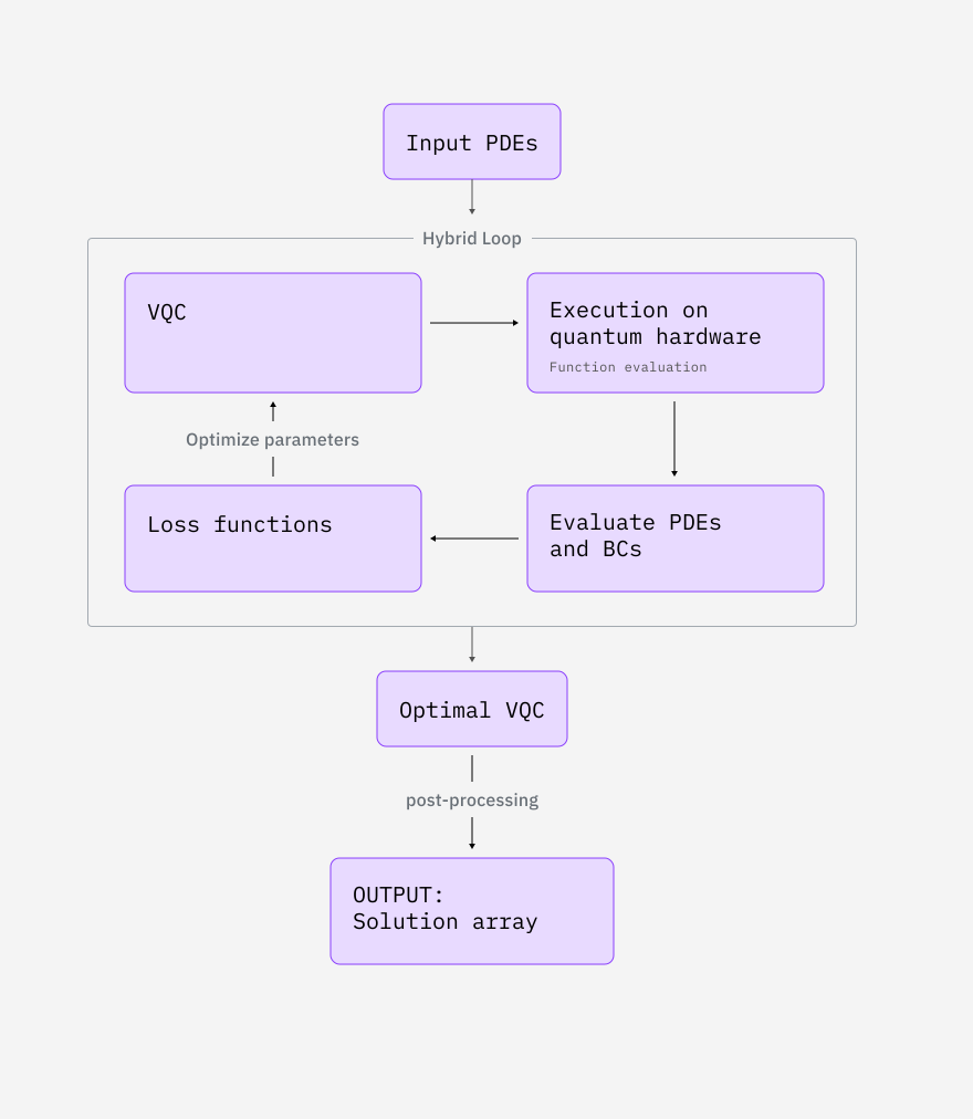
นอกจาก hybrid loop นี้ คุณยังต่อ optimizer หลายตัวเข้าด้วยกันได้ ซึ่งมีประโยชน์เมื่อต้องการ optimizer แบบ global เพื่อหาชุดมุมที่ดี แล้วตามด้วย optimizer ที่ละเอียดกว่าเพื่อไล่ตาม gradient ไปยังชุดมุมที่ดีที่สุดในบริเวณใกล้เคียง ในกรณีของ computational fluid dynamics (CFD) ลำดับการ optimize เริ่มต้นให้ผลลัพธ์ที่ดีที่สุด — แต่ในกรณีของ material deformation (MD) แม้ค่าเริ่มต้นจะให้ผลดี คุณก็กำหนดค่าเพิ่มเติมเพื่อประโยชน์เฉพาะปัญหาได้

หมายเหตุ สำหรับตัวแปรแต่ละตัวของฟังก์ชัน เราระบุจำนวน qubits (ซึ่งคุณปรับเปลี่ยนได้) โดยการซ้อน 10 Circuit เหมือนกันและประเมิน 10 observable เหมือนกันบน qubits ที่ต่างกันตลอด Circuit ใหญ่หนึ่ง Circuit คุณลด noise ภายในกระบวนการ CMA optimization ได้ โดยอาศัยวิธี noise learner และลดจำนวน shots ที่ต้องการอย่างมีนัยสำคัญ

พลศาสตร์ของไหลเชิงคำนวณ

สมการ Burgers' แบบ inviscid สร้างแบบจำลองของไหลไม่มีความหนืดที่ไหลดังนี้:

$\frac{\partial u}{\partial t} + u\frac{\partial u}{\partial x} = 0,$

$u$ แทนฟิลด์ความเร็วของของไหล กรณีการใช้งานนี้มีเงื่อนไขขอบเขตทางเวลา: คุณเลือกเงื่อนไขเริ่มต้นและปล่อยให้ระบบผ่อนคลาย ปัจจุบันเงื่อนไขเริ่มต้นที่ยอมรับได้มีเพียงฟังก์ชันเชิงเส้น: $ax + b$ วิธีแก้เชิงวิเคราะห์คือ:

$u(t, x) = \frac{ax + b}{at + 1}.$

สมการ pressureless Euler จำลองการไหลของของไหลแบบ inviscid ที่บีบอัดได้พร้อมการหน่วง ดังนี้:

$\frac{\partial g}{\partial t} + u\frac{\partial g}{\partial x} + g\frac{\partial u}{\partial x} = 0,$

$u\frac{\partial g}{\partial t} + g\frac{\partial u}{\partial t} + u^2\frac{\partial g}{\partial x} + 2gu\frac{\partial u}{\partial x} + \frac{\mu}{(1+t)^{\lambda}} g u = 0,$

$g$ แทน density field, $u$ แทน velocity field และ $\mu$ แทนสัมประสิทธิ์การหน่วง ในสูตรของเรา เรากำหนด $\lambda = 1$ ดังนั้นจะไม่ถูกใช้เป็นพารามิเตอร์ต่อไป กรณีใช้งานนี้มีเงื่อนไขขอบเขตเชิงเวลา: $g(0, x) = e^{-x}$ และ $u(0, x) = x$ คำตอบเชิงวิเคราะห์คือ:

$g(t, x) = \frac{1-\mu}{(1+t)^{1-\mu} - \mu} \exp\!\left(\frac{(\mu-1)\, x}{(1+t)^{1-\mu} - \mu}\right),$

$u(t, x) = \frac{(1-\mu)\, x}{\left((1+t)^{1-\mu} - \mu\right)(1+t)^{\mu}}.$

อาร์กิวเมนต์สำหรับสมการอนุพันธ์ของ CFD อยู่บน grid คงที่ ดังนี้:

• $t$ อยู่ระหว่าง 0 ถึง 0.95 พร้อม 41 จุดตัวอย่าง $x$ อยู่ระหว่าง 0 ถึง 0.95 พร้อม 41 จุดตัวอย่าง

Material Deformation

กรณีการใช้งานนี้เน้นที่การเสียรูปแบบ hypoelastic ด้วยการทดสอบแรงดึงแบบ 1 มิติ ซึ่งแท่งที่ตรึงอยู่ในพื้นที่ถูกดึงที่ปลายอีกด้าน เราอธิบายปัญหาดังนี้:

$u' - \frac{\sigma}{3K} - \frac{2}{\sqrt{3}}\epsilon_0\left(\frac{\sigma'}{\sigma_0\sqrt{3}}\right)^n = 0,$

$\sigma' - b = 0,$

$K$ แทน bulk modulus ของวัสดุที่ถูกยืด $n$ ตัวชี้กำลังของ power law $b$ แรงต่อมวลหน่วย $\epsilon_0$ ขีดจำกัด proportional stress $\sigma_0$ ขีดจำกัด proportional strain $u$ ฟังก์ชัน stress และ $\sigma$ ฟังก์ชัน strain วิธีแก้เชิงวิเคราะห์คือ:

$\sigma(x) = \sigma_0 - bx,$

$u(x) = -\frac{3^{-(3+n)/2}}{2bK(1+n)\,\sigma_0^{n}}\Biggl[3^{(1+n)/2}b^2\sigma_0^n(1+n)x^2 - 2\cdot 3^{(1+n)/2}b\sigma_0^n(1+n)\sigma_0 x - 12\epsilon_0 K\sigma_0^{1+n}$ $- 12b\epsilon_0 K\sigma_0^n x\left(\frac{-bx+\sigma_0}{\sigma_0}\right)^n + 12\epsilon_0 K\sigma_0^{n+1}\left(\frac{-bx+\sigma_0}{\sigma_0}\right)^n - 12\epsilon_0 K \sigma_0^{1+n}\Biggr],$

โดยที่ $\sigma_0 = g(0)$ คือเงื่อนไขขอบเขตของความเครียด (strain) ที่ $x=0$

แท่งที่พิจารณามีความยาวหนึ่งหน่วย กรณีการใช้งานนี้มีเงื่อนไขขอบเขตสำหรับ surface stress $t$ หรือปริมาณงานที่ต้องการเพื่อยืดแท่ง

อาร์กิวเมนต์สำหรับสมการอนุพันธ์ของ MD อยู่บน grid คงที่ ดังนี้:

• $x$ อยู่ระหว่าง 0 ถึง 1 พร้อม 30 จุดตัวอย่าง

Benchmarks

ตารางต่อไปนี้แสดงสถิติจากการรันฟังก์ชันของเราในหลายครั้ง

ตัวอย่าง	จำนวน qubits	Initialization	Error	เวลารวม (นาที)	Runtime usage (นาที)
สมการ Burgers' แบบ inviscid	50	PHYSICALLY_INFORMED	$10^{-2}$	66	25
สมการ pressureless Euler's	70	PHYSICALLY_INFORMED	$10^{-2}$	48	34
Hypoelastic 1D tensile test	18	RANDOM	$10^{-2}$	123	100

เริ่มต้นใช้งาน

กรอก แบบฟอร์มเพื่อขอเข้าถึงฟังก์ชัน QUICK-PDE จากนั้น สมมติว่า บันทึกบัญชีของคุณแล้ว ไว้ใน local environment ให้เลือกฟังก์ชันดังนี้:

# Added by doQumentation — required packages for this notebook
!pip install -q matplotlib numpy qiskit-ibm-catalog

from qiskit_ibm_catalog import QiskitFunctionsCatalog

catalog = QiskitFunctionsCatalog(
    channel="ibm_cloud / ibm_quantum_platform",
    instance="USER_CRN / HGP",
    token="USER_API_KEY / IQP_API_TOKEN",
)

catalog = QiskitFunctionsCatalog(channel="ibm_quantum_platform")

# Verify that you have access to the function
catalog.list()

quick = catalog.load("colibritd/quick-pde")

ตัวอย่าง

ในการเริ่มต้น ลองทำหนึ่งในตัวอย่างต่อไปนี้:

สมการ Burgers' แบบ inviscid (CFD)

สำหรับสมการ Burgers' เมื่อเงื่อนไขเริ่มต้นตั้งเป็น $u(0,x) = x$ ผลลัพธ์มีดังนี้:

# launch the simulation with initial conditions u(0,x) = a*x + b
job = quick.run(
    use_case="CFD_BURGER", physical_parameters={"a": 1.0, "b": 0.0}
)

ตรวจสอบ status ของ Qiskit Function workload หรือดึง ผลลัพธ์ ดังนี้:

# Print the ID so you can use it later, if necessary
print(job.job_id)
print(job.status())
solution = job.result()

import numpy as np
import matplotlib.pyplot as plt

def plot_result_3d(result):
    fig = plt.figure()
    ax = fig.add_subplot(projection="3d")

    t, x = np.meshgrid(result["samples"]["t"], result["samples"]["x"])

    ax.plot_surface(
        t,
        x,
        result["functions"]["u"],
        edgecolor="royalblue",
        lw=0.25,
        rstride=26,
        cstride=26,
        alpha=0.3,
    )
    ax.scatter(t, x, result["functions"]["u"], marker=".")
    ax.set(xlabel="t", ylabel="x", zlabel="u(t,x)")

    plt.show()

# Call
plot_result_3d(solution)

สมการ pressureless Euler's (CFD)

สำหรับสมการ Euler's เมื่อเงื่อนไขเริ่มต้นตั้งเป็น $g(0, x) = e^{-x}$ และ $u(0, x) = x$ สำหรับ $\mu$ ที่กำหนด (ในที่นี้ $\mu = 0.1$) และ $\lambda = 1$ ผลลัพธ์มีดังนี้:

# Launches the solving for an arbitrary mu
job = quick.run(use_case="CFD_EULER", physical_parameters={"mu": 0.1})

solution = job.result()

# Colorplot function
def plot_result_2d(result):
    fig, axes = plt.subplots(1, 2, figsize=(14, 5))

    configs = {
        "g": {"cmap": "viridis", "title": "g(t, x)"},
        "u": {"cmap": "plasma", "title": "u(t, x)"},
    }

    t = result["samples"]["t"]
    x = result["samples"]["x"]

    for ax, (field, cfg) in zip(axes, configs.items()):
        v = result["functions"][field]

        im = ax.contourf(t, x, v, levels=50, cmap=cfg["cmap"])
        fig.colorbar(im, ax=ax, label=cfg["title"])

        ax.set_xlabel("t")
        ax.set_ylabel("x")
        ax.set_title(cfg["title"], fontsize=13, fontweight="bold")

    plt.tight_layout()
    plt.show()

plot_result_2d(solution)

Material Deformation

กรณีการใช้งาน material deformation ต้องการพารามิเตอร์ทางกายภาพของวัสดุและแรงที่ใช้ ดังนี้:

# Select the properties of your material
job = quick.run(
    use_case="MD",
    physical_parameters={
        "t": 12.0,
        "K": 100.0,
        "n": 4.0,
        "b": 10.0,
        "epsilon_0": 0.1,
        "sigma_0": 5.0,
    },
)

# Plot the result
solution = job.result()

_ = plt.figure()
stress_plot = plt.subplot(211)
plt.plot(solution["samples"]["x"], solution["functions"]["u"])
strain_plot = plt.subplot(212)
plt.plot(solution["samples"]["x"], solution["functions"]["sigma"])

plt.show()

ต่อไปนี้เป็นตัวอย่างวิธีรับค่าของฟังก์ชันสำหรับชุดพิกัดเฉพาะ:

# u(t=0.2, x=0.7) == 2
assert solution["samples"]["t"][1] == 0.2
assert solution["samples"]["x"][2] == 0.7
assert solution["functions"]["u"][1, 2] == 2

ดึงข้อความ error

ถ้าสถานะ workload เป็น ERROR ให้ใช้ job.error_message() เพื่อดึงข้อความ error มาช่วย debug ดังนี้:

job = quick.run(use_case="MD", physical_params={})

print(job.error_message())

# A wrapper can also be used for a more human readable version
def pprint_error(job):
    print("".join(eval(job.error_message())["error"]))

print("___")
pprint_error(job)

รับการสนับสนุน

สำหรับการสนับสนุน ติดต่อ qiskit-function-support@colibritd.com

ขั้นตอนถัดไป

คำแนะนำ

• กรอกแบบฟอร์มเพื่อ ขอเข้าถึงฟังก์ชัน QUICK-PDE
• เยี่ยมชม API reference สำหรับ Qiskit Function นี้
• ลองสร้างแบบจำลองของไหลไม่มีความหนืดโดยใช้ QUICK-PDE ใน tutorial
• อ่าน Jaffali, H., et al. (2025). H-DES: a Quantum-Classical Hybrid Differential Equation Solver. arXiv preprint arXiv:2410.01130.