Singularity Machine Learning - Classification: A Qiskit Function by Multiverse Computing

See the API reference

Package versions

The code on this page was developed using the following requirements. We recommend using these versions or newer.

scikit-learn~=1.8.0

Note

• Qiskit Functions เป็นฟีเจอร์ทดลองที่ให้บริการเฉพาะผู้ใช้แผน IBM Quantum® Premium Plan, Flex Plan และ On-Prem (ผ่าน IBM Quantum Platform API) เท่านั้น อยู่ในสถานะ preview release และอาจมีการเปลี่ยนแปลงได้

ภาพรวม

ด้วยฟังก์ชัน "Singularity Machine Learning - Classification" คุณสามารถแก้ปัญหา machine learning ในโลกจริงบน quantum hardware ได้โดยไม่ต้องมีความเชี่ยวชาญด้าน quantum ฟังก์ชัน Application นี้อิงจาก ensemble methods และเป็น hybrid classifier ที่ใช้ประโยชน์จากวิธีแบบคลาสสิก เช่น boosting, bagging และ stacking สำหรับการฝึก ensemble เบื้องต้น จากนั้นจึงนำ quantum algorithms อย่าง variational quantum eigensolver (VQE) และ quantum approximate optimization algorithm (QAOA) มาใช้เพื่อเพิ่มความหลากหลาย ความสามารถในการ generalization และความซับซ้อนโดยรวมของ ensemble ที่ฝึกแล้ว

ต่างจาก quantum machine learning อื่น ๆ ฟังก์ชันนี้สามารถจัดการชุดข้อมูลขนาดใหญ่ที่มีตัวอย่างและ feature หลายล้านรายการได้ โดยไม่ถูกจำกัดด้วยจำนวน Qubit ใน QPU เป้าหมาย จำนวน Qubit จะกำหนดแค่ขนาดของ ensemble ที่สามารถฝึกได้เท่านั้น ฟังก์ชันนี้ยังมีความยืดหยุ่นสูง และสามารถใช้แก้ปัญหา classification ในหลากหลายโดเมน ทั้งด้านการเงิน สาธารณสุข และความปลอดภัยทางไซเบอร์ มันสามารถทำความแม่นยำสูงอย่างสม่ำเสมอบนปัญหาที่ท้าทายสำหรับคอมพิวเตอร์แบบคลาสสิก ซึ่งมีข้อมูลมิติสูง มีสัญญาณรบกวน และมีความไม่สมดุลของคลาส เหมาะสำหรับ:

1. วิศวกรและนักวิทยาศาสตร์ข้อมูลในบริษัทที่ต้องการยกระดับผลิตภัณฑ์และบริการด้วยการนำ quantum machine learning มาผสานรวม
2. นักวิจัยในห้องปฏิบัติการวิจัย quantum ที่กำลังสำรวจการประยุกต์ใช้ quantum machine learning และต้องการใช้ quantum computing สำหรับงาน classification และ
3. นักศึกษาและอาจารย์ในสถาบันการศึกษาในรายวิชา machine learning ที่ต้องการแสดงให้เห็นถึงข้อได้เปรียบของ quantum computing

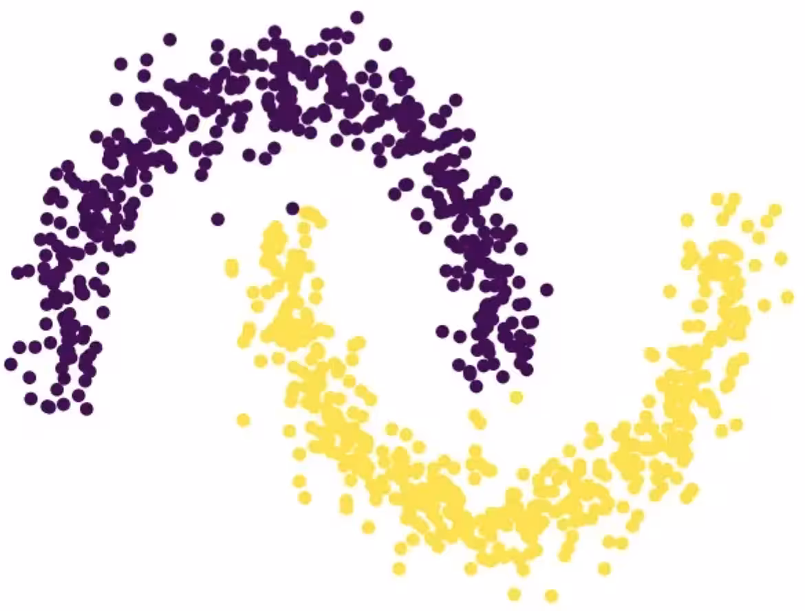
ตัวอย่างต่อไปนี้แสดงฟังก์ชันต่าง ๆ ของมัน ได้แก่ create, list, fit และ predict และแสดงวิธีใช้งานกับปัญหาสังเคราะห์ที่ประกอบด้วยครึ่งวงกลมสองอันเชื่อมต่อกัน ซึ่งเป็นปัญหาที่ท้าทายอย่างมากเนื่องจาก decision boundary ที่ไม่เป็นเส้นตรง

คำอธิบายฟังก์ชัน

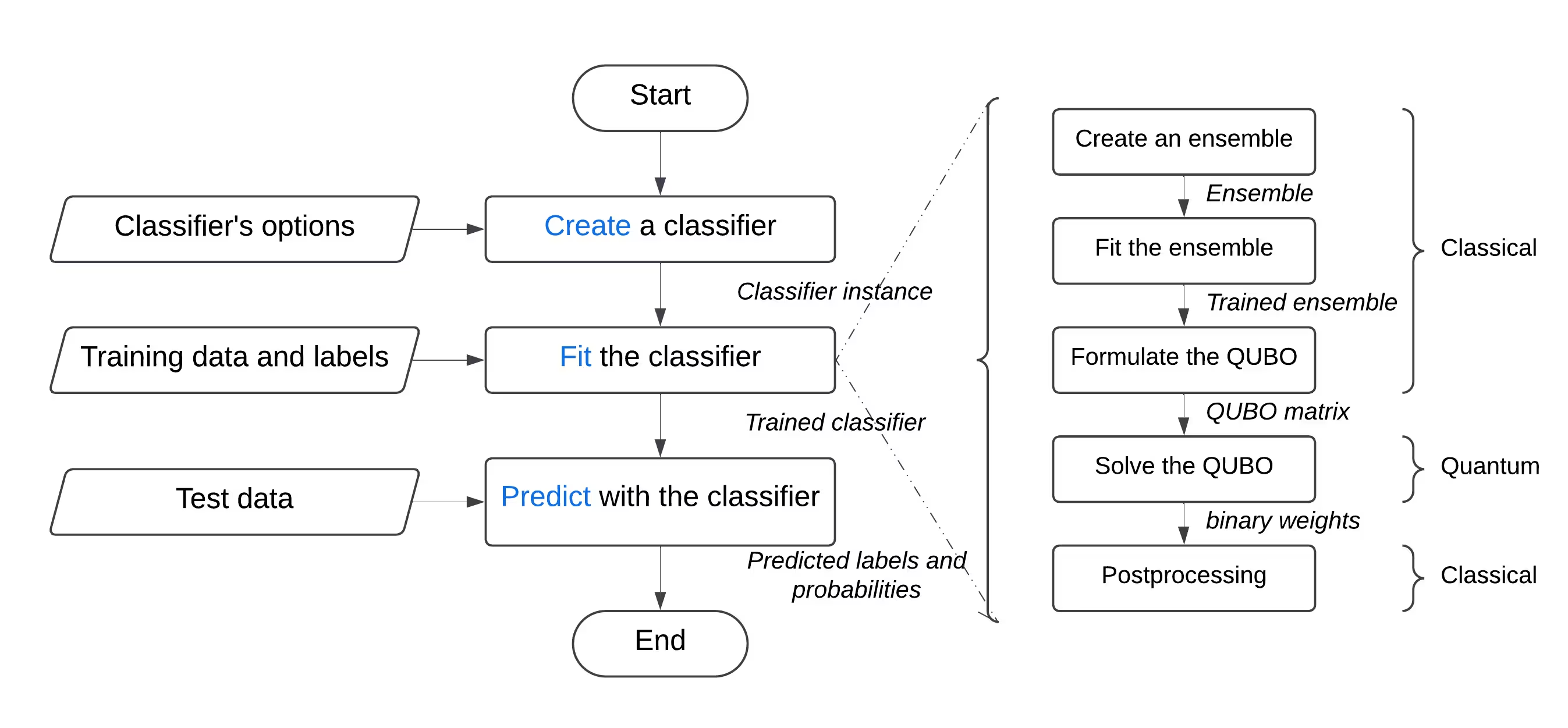
Qiskit Function นี้ช่วยให้ผู้ใช้สามารถแก้ปัญหา binary classification โดยใช้ quantum-enhanced ensemble classifier ของ Singularity เบื้องหลัง มันใช้แนวทาง hybrid ในการฝึก ensemble ของ classifier แบบคลาสสิกบนชุดข้อมูลที่มี label แล้วปรับแต่งให้มีความหลากหลายและ generalization สูงสุดโดยใช้ Quantum Approximate Optimization Algorithm (QAOA) บน IBM® QPUs ผ่านอินเตอร์เฟซที่ใช้งานง่าย ผู้ใช้สามารถกำหนดค่า classifier ตามความต้องการ ฝึกมันบนชุดข้อมูลที่เลือก และใช้มันทำนายผลบนชุดข้อมูลที่ไม่เคยเห็นมาก่อน

เพื่อแก้ปัญหา classification ทั่วไป:

1. ประมวลผลชุดข้อมูลล่วงหน้า และแบ่งออกเป็นชุดฝึกและชุดทดสอบ ถ้าต้องการ สามารถแบ่งชุดฝึกออกเป็นชุดฝึกและชุด validation เพิ่มเติมได้ ทำได้โดยใช้ scikit-learn
2. ถ้าชุดฝึกไม่สมดุล คุณสามารถทำการ resample เพื่อปรับสมดุลของคลาสได้โดยใช้ imbalanced-learn
3. อัปโหลดชุดฝึก ชุด validation และชุดทดสอบแยกกันไปยัง storage ของฟังก์ชัน โดยใช้เมธอด file_upload ของ catalog และส่ง path ที่เกี่ยวข้องในแต่ละครั้ง
4. เริ่มต้น quantum classifier โดยใช้ action create ของฟังก์ชัน ซึ่งรับ hyperparameter ต่าง ๆ เช่น จำนวนและประเภทของ learner, regularization (ค่า lambda) และตัวเลือกการ optimization รวมถึงจำนวน layer, ประเภทของ classical optimizer, quantum Backend และอื่น ๆ
5. ฝึก quantum classifier บนชุดฝึกโดยใช้ action fit ของฟังก์ชัน โดยส่งชุดฝึกที่มี label และชุด validation (ถ้ามี)
6. ทำนายผลบนชุดทดสอบที่ไม่เคยเห็นมาก่อนโดยใช้ action predict ของฟังก์ชัน

---

Get started

ยืนยันตัวตนด้วย IBM Quantum Platform API key แล้วเลือก Qiskit Function ดังนี้:

# Added by doQumentation — required packages for this notebook
!pip install -q numpy qiskit-ibm-catalog scikit-learn

from qiskit_ibm_catalog import QiskitFunctionsCatalog

catalog = QiskitFunctionsCatalog(channel="ibm_quantum_platform")

# load function
singularity = catalog.load("multiverse/singularity")

Examples

Classify a dataset

ในตัวอย่างนี้ เราจะใช้ฟังก์ชัน "Singularity Machine Learning - Classification" เพื่อจำแนกชุดข้อมูลที่ประกอบด้วยครึ่งวงกลมสองอันที่พันกันเป็นรูปพระจันทร์เสี้ยว ชุดข้อมูลนี้เป็นชุดสังเคราะห์ สองมิติ และมีป้ายกำกับแบบไบนารี ออกแบบมาให้ท้าทายกับอัลกอริทึม เช่น การจัดกลุ่มแบบ centroid-based และการจำแนกเชิงเส้น ในกระบวนการนี้ เราจะเรียนรู้วิธีสร้าง classifier, fit กับข้อมูล training, ใช้ทำนายข้อมูล test และลบ classifier เมื่อใช้งานเสร็จ ก่อนเริ่มต้น ต้องติดตั้ง scikit-learn ก่อน ติดตั้งด้วยคำสั่งต่อไปนี้:

python3 -m pip install scikit-learn

ทำตามขั้นตอนต่อไปนี้:

1. สร้างชุดข้อมูลสังเคราะห์โดยใช้ฟังก์ชัน make_moons จาก scikit-learn
2. อัปโหลดชุดข้อมูลสังเคราะห์ที่สร้างขึ้นไปยัง shared data directory
3. สร้าง quantum-enhanced classifier โดยใช้ action create
4. ดูรายการ classifier ของคุณโดยใช้ action list
5. เทรน classifier ด้วยข้อมูล train โดยใช้ action fit
6. ใช้ classifier ที่เทรนแล้วเพื่อทำนายข้อมูล test โดยใช้ action predict
7. ลบ classifier โดยใช้ action delete
8. ล้างข้อมูลเมื่อทำเสร็จแล้ว

ขั้นตอนที่ 1. นำเข้าโมดูลที่จำเป็นและสร้างชุดข้อมูลสังเคราะห์ จากนั้นแบ่งเป็นชุดข้อมูล training และ test

# import the necessary modules for this example
import os
import tarfile
import numpy as np

# Import the make_moons and the train_test_split functions from scikit-learn
# to create a synthetic dataset and split it into training and test datasets
from sklearn.datasets import make_moons
from sklearn.model_selection import train_test_split

# generate the synthetic dataset
X, y = make_moons(n_samples=10000)

# split the data into training and test datasets
X_train, X_test, y_train, y_test = train_test_split(X, y, test_size=0.2)

# print the first 10 samples of the training dataset
print("Features:", X_train[:10, :])
print("Targets:", y_train[:10])

Features: [[ 0.84757037 -0.48831433]
 [ 0.98132552  0.19235443]
 [-0.71626723  0.6978261 ]
 [ 1.18957848 -0.48186557]
 [ 0.52118982 -0.37791846]
 [ 0.81115408  0.58483251]
 [ 0.48706462  0.87336593]
 [-0.81880144  0.57407682]
 [ 1.67335408 -0.23932015]
 [ 0.50181306  0.8649761 ]]
Targets: [1 0 0 1 1 0 0 0 1 0]

ขั้นตอนที่ 2. บันทึกชุดข้อมูล training และ test ที่มีป้ายกำกับลงในดิสก์ในเครื่อง จากนั้นอัปโหลดไปยัง shared data directory

def make_tarfile(file_path, tar_file_name):
    with tarfile.open(tar_file_name, "w") as tar:
        tar.add(file_path, arcname=os.path.basename(file_path))

# save the training and test datasets on your local disk
np.save("X_train.npy", X_train)
np.save("y_train.npy", y_train)
np.save("X_test.npy", X_test)
np.save("y_test.npy", y_test)

# create tar files for the datasets
make_tarfile("X_train.npy", "X_train.npy.tar")
make_tarfile("y_train.npy", "y_train.npy.tar")
make_tarfile("X_test.npy", "X_test.npy.tar")
make_tarfile("y_test.npy", "y_test.npy.tar")

# upload the datasets to the shared data directory
catalog.file_upload("X_train.npy.tar", singularity)
catalog.file_upload("y_train.npy.tar", singularity)
catalog.file_upload("X_test.npy.tar", singularity)
catalog.file_upload("y_test.npy.tar", singularity)

# view/enlist the uploaded files in the shared data directory
print(catalog.files(singularity))

['X_test.npy.tar', 'X_train.npy.tar', 'y_test.npy.tar', 'y_train.npy.tar']

ขั้นตอนที่ 3. สร้าง quantum-enhanced classifier โดยใช้ action create

job = singularity.run(
    action="create",
    name="my_classifier",
    num_learners=10,
    learners_types=[
        "DecisionTreeClassifier",
        "KNeighborsClassifier",
    ],
    learners_proportions=[0.5, 0.5],
    learners_options=[{}, {}],
    regularization=0.01,
    weight_update_method="logarithmic",
    sample_scaling=True,
    optimizer_options={"simulator": True},
    voting="soft",
    prob_threshold=0.5,
)

print(job.result())

{'status': 'ok', 'message': 'Classifier created.', 'data': {}, 'metadata': {'resource_usage': {}}}

# list available classifiers using the list action
job = singularity.run(action="list")

print(job.result())

# you can also find your classifiers in the shared data directory with a *.pkl.tar extension
print(catalog.files(singularity))

{'status': 'ok', 'message': 'Classifiers listed.', 'data': {'classifiers': ['my_classifier']}, 'metadata': {'resource_usage': {}}}

['X_test.npy.tar', 'X_train.npy.tar', 'my_classifier.pkl.tar', 'y_test.npy.tar', 'y_train.npy.tar']

ขั้นตอนที่ 4. เทรน quantum-enhanced classifier โดยใช้ action fit

job = singularity.run(
    action="fit",
    name="my_classifier",
    X="X_train.npy",  # you do not need to specify the tar extension
    y="y_train.npy",  # you do not need to specify the tar extension
)

print(job.result())

{'status': 'ok', 'message': 'Classifier fitted.', 'data': {}, 'metadata': {'resource_usage': {'RUNNING: MAPPING': {'CPU_TIME': 13.655871629714966}, 'RUNNING: WAITING_QPU': {'CPU_TIME': 54.688621282577515}, 'RUNNING: POST_PROCESSING': {'CPU_TIME': 56.92286920547485}, 'RUNNING: EXECUTING_QPU': {'QPU_TIME': 57.92738223075867}}}}

ขั้นตอนที่ 5. รับผลการทำนายและความน่าจะเป็นจาก quantum-enhanced classifier โดยใช้ action predict

job = singularity.run(
    action="predict",
    name="my_classifier",
    X="X_test.npy",  # you do not need to specify the tar extension
)

result = job.result()

print("Action result status: ", result["status"])
print("Action result message: ", result["message"])
print("Predictions (first five results):", result["data"]["predictions"][:5])
print(
    "Probabilities (first five results):", result["data"]["probabilities"][:5]
)

Action result status:  ok
Action result message:  Classifier predicted.
Predictions (first five results): [0, 0, 1, 0, 1]
Probabilities (first five results): [[1.0, 0.0], [1.0, 0.0], [0.0, 1.0], [1.0, 0.0], [0.0, 1.0]]

ขั้นตอนที่ 6. ลบ quantum-enhanced classifier โดยใช้ action delete

job = singularity.run(
    action="delete",
    name="my_classifier",
)

# or you can delete from the shared data directory
# catalog.file_delete("my_classifier.pkl.tar", singularity)

print(job.result())

{'status': 'ok', 'message': 'Classifier deleted.', 'data': {}, 'metadata': {'resource_usage': {}}}

ขั้นตอนที่ 7. ล้างข้อมูลในไดเรกทอรีในเครื่องและไดเรกทอรีข้อมูลที่แชร์

# delete the numpy files from your local disk
os.remove("X_train.npy")
os.remove("y_train.npy")
os.remove("X_test.npy")
os.remove("y_test.npy")

# delete the tar files from your local disk
os.remove("X_train.npy.tar")
os.remove("y_train.npy.tar")
os.remove("X_test.npy.tar")
os.remove("y_test.npy.tar")

# delete the tar files from the shared data
catalog.file_delete("X_train.npy.tar", singularity)
catalog.file_delete("y_train.npy.tar", singularity)
catalog.file_delete("X_test.npy.tar", singularity)
catalog.file_delete("y_test.npy.tar", singularity)

'Requested file was deleted.'

ตัวอย่าง create_fit_predict

ตัวอย่างต่อไปนี้แสดงการใช้งาน action create_fit_predict

# Import QiskitFunctionsCatalog to load the
# "Singularity Machine Learning - Classification" function by Multiverse Computing
from qiskit_ibm_catalog import QiskitFunctionsCatalog

# Import the make_moons and the train_test_split functions from scikit-learn
# to create a synthetic dataset and split it into training and test datasets
from sklearn.datasets import make_moons
from sklearn.model_selection import train_test_split

# authentication
# If you have not previously saved your credentials, follow instructions at
# /docs/guides/functions
# to authenticate with your API key.
catalog = QiskitFunctionsCatalog(channel="ibm_quantum_platform")

# load "Singularity Machine Learning - Classification" function by Multiverse Computing
singularity = catalog.load("multiverse/singularity")

# generate the synthetic dataset
X, y = make_moons(n_samples=1000)

# split the data into training and test datasets
X_train, X_test, y_train, y_test = train_test_split(X, y, test_size=0.2)

job = singularity.run(
    action="create_fit_predict",
    num_learners=10,
    regularization=0.01,
    optimizer_options={"simulator": True},
    X_train=X_train,
    y_train=y_train,
    X_test=X_test,
    options={"save": False},
)

# get job status and result
status = job.status()
result = job.result()

print("Job status: ", status)
print("Action result status: ", result["status"])
print("Action result message: ", result["message"])
print("Predictions (first five results): ", result["data"]["predictions"][:5])
print(
    "Probabilities (first five results): ",
    result["data"]["probabilities"][:5],
)
print("Usage metadata: ", result["metadata"]["resource_usage"])

Job status:  QUEUED
Action result status:  ok
Action result message:  Classifier created, fitted, and predicted.
Predictions (first five results):  [0, 0, 1, 0, 0]
Probabilities (first five results):  [[0.87119766531518, 0.1288023346848197], [0.87119766531518, 0.1288023346848197], [0.24470328446479797, 0.7552967155352032], [0.820524432250189, 0.17947556774981072], [0.6847610293419495, 0.31523897065805173]]
Usage metadata:  {'RUNNING: MAPPING': {'CPU_TIME': 10.967791318893433}, 'RUNNING: WAITING_QPU': {'CPU_TIME': 59.91712307929993}, 'RUNNING: POST_PROCESSING': {'CPU_TIME': 59.097386837005615}, 'RUNNING: EXECUTING_QPU': {'QPU_TIME': 56.93338203430176}}

Benchmarks

Benchmarks เหล่านี้แสดงให้เห็นว่า classifier สามารถบรรลุความแม่นยำสูงมากบนปัญหาที่ท้าทายได้ นอกจากนี้ยังแสดงให้เห็นว่าการเพิ่มจำนวน learner ใน ensemble (จำนวน Qubit) สามารถนำไปสู่ความแม่นยำที่เพิ่มขึ้นได้

"Classical accuracy" หมายถึงความแม่นยำที่ได้จากการใช้ state of the art แบบ classical ที่สอดคล้องกัน ซึ่งในกรณีนี้คือ AdaBoost classifier ที่อิงบน ensemble ขนาด 75 ส่วน "Quantum accuracy" หมายถึงความแม่นยำที่ได้จากการใช้ "Singularity Machine Learning - Classification"

ปัญหา	ขนาด Dataset	ขนาด Ensemble	จำนวน Qubit	ความแม่นยำแบบ Classical	ความแม่นยำแบบ Quantum	การปรับปรุง
Grid stability	5000 ตัวอย่าง, 12 features	55	55	76%	91%	15%
Grid stability	5000 ตัวอย่าง, 12 features	65	65	76%	92%	16%
Grid stability	5000 ตัวอย่าง, 12 features	75	75	76%	94%	18%
Grid stability	5000 ตัวอย่าง, 12 features	85	85	76%	94%	18%
Grid stability	5000 ตัวอย่าง, 12 features	100	100	76%	95%	19%

---

เมื่อ hardware ของ quantum พัฒนาและขยายขนาดขึ้น ผลกระทบต่อ quantum classifier ของเราก็มีความสำคัญมากขึ้นเรื่อยๆ แม้ว่าจำนวน Qubit จะกำหนดข้อจำกัดในขนาดของ ensemble ที่สามารถใช้ได้ แต่ก็ไม่ได้จำกัดปริมาณข้อมูลที่สามารถประมวลผลได้ ความสามารถอันทรงพลังนี้ทำให้ classifier สามารถจัดการ dataset ที่มีข้อมูลหลายล้านจุดและ features หลายพันรายการได้อย่างมีประสิทธิภาพ สิ่งสำคัญคือข้อจำกัดที่เกี่ยวข้องกับขนาด ensemble สามารถแก้ไขได้ผ่านการนำ classifier เวอร์ชันขนาดใหญ่มาใช้ การใช้ประโยชน์จากแนวทาง iterative outer-loop ทำให้ ensemble สามารถขยายขนาดได้แบบ dynamic เพิ่มความยืดหยุ่นและประสิทธิภาพโดยรวม อย่างไรก็ตาม ควรทราบว่าฟีเจอร์นี้ยังไม่ได้ถูกนำมาใช้ในเวอร์ชันปัจจุบันของ classifier

Changelog

4 มิถุนายน 2025

• อัปเกรด QuantumEnhancedEnsembleClassifier ด้วยการอัปเดตดังต่อไปนี้:
  • เพิ่ม onsite/alpha regularization สามารถกำหนด regularization_type เป็น onsite หรือ alpha ได้
  • เพิ่ม auto-regularization สามารถตั้ง regularization เป็น auto เพื่อใช้ auto-regularization
  • เพิ่มพารามิเตอร์ optimization_data ใน method fit เพื่อเลือกข้อมูลสำหรับ quantum optimization สามารถใช้หนึ่งในตัวเลือกเหล่านี้: train, validation, หรือ both
  • ปรับปรุงประสิทธิภาพโดยรวม
• เพิ่มการติดตามสถานะอย่างละเอียดสำหรับ job ที่กำลังทำงาน

20 พฤษภาคม 2025

• ปรับมาตรฐานการจัดการข้อผิดพลาด

18 มีนาคม 2025

• อัปเกรด qiskit-serverless เป็น 0.20.0 และ base image เป็น 0.20.1

14 กุมภาพันธ์ 2025

• อัปเกรด base image เป็น 0.19.1

6 กุมภาพันธ์ 2025

• อัปเกรด qiskit-serverless เป็น 0.19.0 และ base image เป็น 0.19.0

13 พฤศจิกายน 2024

• เปิดตัว Singularity Machine Learning - Classification

Get support

สำหรับคำถามใดๆ ติดต่อ Multiverse Computing

อย่าลืมใส่ข้อมูลต่อไปนี้:

• Qiskit Function Job ID (job.job_id)
• คำอธิบายปัญหาอย่างละเอียด
• ข้อความหรือรหัสข้อผิดพลาดที่เกี่ยวข้อง
• ขั้นตอนในการทำซ้ำปัญหา

Next steps

คำแนะนำ

• ขอสิทธิ์เข้าถึง Multiverse Computing's Singularity Machine Learning Classification function.
• เยี่ยมชม API reference สำหรับ Qiskit Function นี้
• อ่าน Leclerc, L., et al. (2023). Financial risk management on a neutral atom quantum processor. Physical Review Research, 5, 043117