การใช้งาน Qiskit

ในบทเรียนนี้ เราจะนำแนวคิดบางส่วนจากบทเรียนเรื่อง entanglement in action มาสู่การปฏิบัติโดยใช้ Qiskit

# Added by doQumentation — required packages for this notebook
!pip install -q qiskit qiskit-aer

from qiskit import __version__

print(__version__)

2.1.1

from qiskit import QuantumCircuit, QuantumRegister, ClassicalRegister
from qiskit_aer import AerSimulator
from qiskit.visualization import plot_histogram, array_to_latex
from qiskit.result import marginal_distribution
from qiskit.circuit.library import UGate
from math import pi
import random

ต่อไปนี้คือการใช้งาน Circuit ควอนตัมของโปรโตคอล teleportation

qubit = QuantumRegister(1, "Q")
ebit0 = QuantumRegister(1, "A")
ebit1 = QuantumRegister(1, "B")
a = ClassicalRegister(1, "a")
b = ClassicalRegister(1, "b")

protocol = QuantumCircuit(qubit, ebit0, ebit1, a, b)

# Prepare ebit used for teleportation
protocol.h(ebit0)
protocol.cx(ebit0, ebit1)
protocol.barrier()

# Alice's operations
protocol.cx(qubit, ebit0)
protocol.h(qubit)
protocol.barrier()

# Alice measures and sends classical bits to Bob
protocol.measure(ebit0, a)
protocol.measure(qubit, b)
protocol.barrier()

# Bob uses the classical bits to conditionally apply gates
with protocol.if_test((a, 1)):
    protocol.x(ebit1)
with protocol.if_test((b, 1)):
    protocol.z(ebit1)

display(protocol.draw(output="mpl"))

Circuit นี้ใช้ฟีเจอร์บางอย่างของ Qiskit ที่เราไม่เคยเห็นในบทเรียนก่อนหน้า ได้แก่ฟังก์ชัน barrier และ if_test ฟังก์ชัน barrier สร้างการแบ่งแยกทางภาพทำให้ diagram ของ Circuit อ่านง่ายขึ้น และยังป้องกันไม่ให้ Qiskit ทำการปรับปรุงและ optimize ข้ามบริเวณ barrier ระหว่างการ compile เมื่อรัน Circuit บน hardware จริง ฟังก์ชัน if_test ใช้งาน operation แบบมีเงื่อนไขขึ้นอยู่กับ classical bit หรือ register

Circuit นี้จะเริ่มต้นด้วยการทำให้ $(\mathsf{A},\mathsf{B})$ อยู่ใน state $\vert \phi^+\rangle$ (ซึ่งไม่ได้เป็นส่วนหนึ่งของโปรโตคอลเอง) ตามด้วย operation ของ Alice แล้วจึงเป็นการวัดผล และสุดท้าย operation ของ Bob เพื่อทดสอบว่าโปรโตคอลทำงานได้ถูกต้อง เราจะใช้ Gate เดี่ยว-Qubit ที่สร้างแบบสุ่มกับ state $\vert 0\rangle$ ที่กำหนดค่าเริ่มต้นของ $\mathsf{Q}$ เพื่อให้ได้ vector state ควอนตัมสุ่มที่จะทำการ teleport จากนั้นโดยการใช้ inverse (คือ conjugate transpose) ของ Gate นั้นกับ $\mathsf{B}$ หลังจากที่รันโปรโตคอลแล้ว เราสามารถตรวจสอบว่า state ถูก teleport ได้สำเร็จโดยวัดเพื่อดูว่ามันกลับมาอยู่ที่ state $\vert 0\rangle$ หรือไม่

ขั้นแรกเราจะสุ่มเลือก Gate Qubit แบบ unitary

random_gate = UGate(
    theta=random.random() * 2 * pi,
    phi=random.random() * 2 * pi,
    lam=random.random() * 2 * pi,
)

display(array_to_latex(random_gate.to_matrix()))

$$\begin{bmatrix} 0.9897212158 & -0.0195080103 - 0.141673401 i \\ 0.0603319186 + 0.1296609988 i & -0.8319925233 + 0.5360378028 i \\ \end{bmatrix}$$

ต่อมาเราจะสร้าง Circuit ทดสอบใหม่ที่ขั้นแรกใช้ Gate สุ่มของเรากับ $\mathsf{Q}$, จากนั้นรัน Circuit teleportation และสุดท้ายใช้ inverse ของ Gate สุ่มของเรากับ Qubit $\mathsf{B}$ แล้ววัดผล ผลลัพธ์ควรเป็น $0$ อย่างแน่นอน

# Create a new circuit including the same bits and qubits used in the
# teleportation protocol.

test = QuantumCircuit(qubit, ebit0, ebit1, a, b)

# Start with the randomly selected gate on Q

test.append(random_gate, qubit)
test.barrier()

# Append the entire teleportation protocol from above.

test = test.compose(protocol)
test.barrier()

# Finally, apply the inverse of the random unitary to B and measure.

test.append(random_gate.inverse(), ebit1)
result = ClassicalRegister(1, "Result")
test.add_register(result)
test.measure(ebit1, result)

display(test.draw(output="mpl"))

สุดท้าย ลองรัน Aer simulator บน Circuit นี้และพล็อต histogram ของผลลัพธ์ เราจะเห็น statistics สำหรับ classical bit ทั้งสามตัว: bit ล่าง/ซ้ายสุดควรเป็น $0$ เสมอ ซึ่งแสดงว่า Qubit $\mathsf{Q}$ ถูก teleport ไปยัง $\mathsf{B}$ สำเร็จ ในขณะที่ bit อีกสองตัวควรสม่ำเสมอโดยประมาณ

result = AerSimulator().run(test).result()
statistics = result.get_counts()
display(plot_histogram(statistics))

เราสามารถกรอง statistics เพื่อโฟกัสเฉพาะที่ Qubit ผลการทดสอบได้หากต้องการ เช่นนี้:

filtered_statistics = marginal_distribution(statistics, [2])
display(plot_histogram(filtered_statistics))

การเข้ารหัสแบบซูเปอร์เดนส์

Superdense coding คือโปรโตคอลที่ในแง่หนึ่งมีเป้าหมายที่เป็น complement กับ teleportation แทนที่จะช่วยให้ส่ง Qubit หนึ่งตัวโดยใช้การสื่อสาร classical bit สองบิต (แลกกับ e-bit ของ entanglement หนึ่งหน่วย) มันอนุญาตให้ส่ง classical bit สองบิตโดยใช้การสื่อสารควอนตัม qubit หนึ่งตัว (อีกครั้งแลกกับ e-bit ของ entanglement หนึ่งหน่วย)

ในรายละเอียดมากขึ้น เรามีผู้ส่ง (Alice) และผู้รับ (Bob) ที่แชร์ e-bit ของ entanglement หนึ่งหน่วย ตามข้อตกลงในบทเรียน นั่นหมายความว่า Alice ถือ Qubit $\mathsf{A}$, Bob ถือ Qubit $\mathsf{B}$, และคู่ $(\mathsf{A},\mathsf{B})$ อยู่ใน state $\vert\phi^+\rangle$ Alice ต้องการส่ง classical bit สองบิตให้ Bob ซึ่งเราจะเรียกว่า $c$ และ $d$, และเธอจะทำสิ่งนี้โดยส่ง Qubit หนึ่งตัวให้เขา

เป็นเรื่องสมเหตุสมผลที่จะมองว่าความสำเร็จนี้น่าสนใจน้อยกว่าสิ่งที่ teleportation ทำได้ การส่ง Qubit นั้นน่าจะยากกว่าการส่ง classical bit มากในอนาคตอันใกล้ ดังนั้นการแลก quantum communication หนึ่ง Qubit กับ classical communication สองบิต โดยแลกกับ e-bit อีกด้วย แทบจะไม่คุ้มค่า อย่างไรก็ตาม สิ่งนี้ไม่ได้หมายความว่า superdense coding ไม่น่าสนใจ เพราะมันน่าสนใจอย่างแน่นอน

สอดคล้องกับธีมของบทเรียน เหตุผลหนึ่งที่ superdense coding น่าสนใจคือมันแสดงให้เห็นถึงการใช้งาน entanglement ที่เป็นรูปธรรมและ (ในบริบทของทฤษฎีสารสนเทศ) ค่อนข้างน่าประทับใจ ทฤษฎีบทที่มีชื่อเสียงในทฤษฎีสารสนเทศควอนตัม ที่รู้จักกันในชื่อ ทฤษฎีบทของ Holevo หมายความว่าหากไม่มีการใช้ state entangled ที่แชร์กัน เป็นไปไม่ได้ที่จะสื่อสาร classical information มากกว่าหนึ่งบิตโดยการส่ง Qubit เดียว (ทฤษฎีบทของ Holevo นั้นมีความทั่วไปมากกว่านี้ ถ้อยความที่แม่นยำนั้นมีความเป็นเทคนิคและต้องการการอธิบาย แต่นี่คือผลลัพธ์หนึ่งของมัน) ดังนั้น ผ่าน superdense coding entanglement ที่แชร์กันช่วยให้ เพิ่มเป็นสองเท่า ของความสามารถในการบรรจุ classical information ของการส่ง Qubit ได้อย่างมีประสิทธิภาพ

โปรโตคอล

Diagram ของ Circuit ควอนตัมต่อไปนี้อธิบายโปรโตคอล superdense coding:

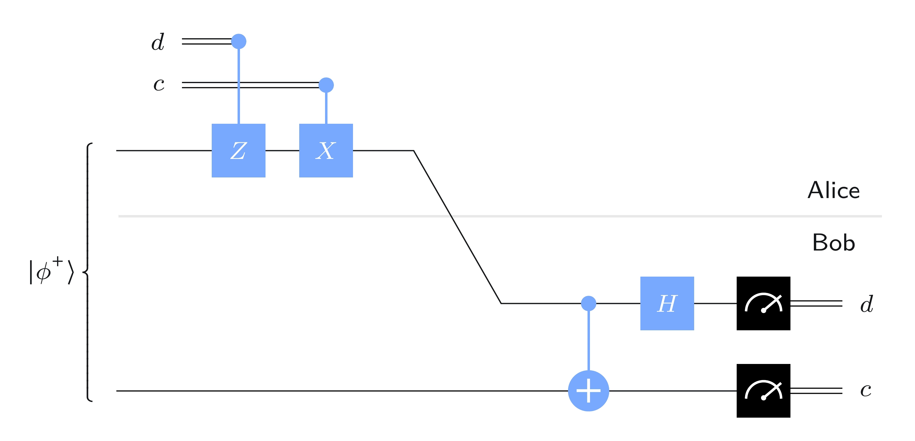
สิ่งที่ Alice ทำในภาษาทั่วไปมีดังนี้:

1. ถ้า $d=1$, Alice ทำ $Z$ Gate กับ Qubit $\mathsf{A}$ ของเธอ (และถ้า $d=0$ เธอไม่ทำ)

2. ถ้า $c=1$, Alice ทำ $X$ Gate กับ Qubit $\mathsf{A}$ ของเธอ (และถ้า $c=0$ เธอไม่ทำ)

จากนั้น Alice ส่ง Qubit $\mathsf{A}$ ของเธอให้ Bob

สิ่งที่ Bob ทำเมื่อได้รับ Qubit $\mathsf{A}$ คือขั้นแรกทำ controlled-NOT Gate โดยให้ $\mathsf{A}$ เป็น control และ $\mathsf{B}$ เป็น target จากนั้นเขาใช้ Hadamard Gate กับ $\mathsf{A}$ จากนั้นเขาวัด $\mathsf{B}$ เพื่อให้ได้ $c$ และวัด $\mathsf{A}$ เพื่อให้ได้ $d$ โดยวัดด้วย standard basis ในทั้งสองกรณี

การวิเคราะห์

แนวคิดเบื้องหลังโปรโตคอลนี้ง่าย: Alice เลือกได้อย่างมีประสิทธิภาพว่าเธอต้องการแชร์ Bell state ใดกับ Bob เธอส่ง Qubit ของเธอให้ Bob และ Bob วัดเพื่อตรวจสอบว่า Alice เลือก Bell state ใด

กล่าวคือ ในตอนแรกพวกเขาแชร์ $\vert\phi^+\rangle$ และขึ้นอยู่กับบิต $c$ และ $d,$ Alice จะปล่อย state นี้ไว้ตามเดิมหรือเปลี่ยนมันไปยัง Bell state อื่นโดยการใช้ $\mathbb{I},$ $X,$ $Z,$ หรือ $XZ$ กับ Qubit $\mathsf{A}$ ของเธอ

$$\begin{aligned} (\mathbb{I} \otimes \mathbb{I}) \vert \phi^+ \rangle & = \vert \phi^+\rangle \\ (\mathbb{I} \otimes Z) \vert \phi^+ \rangle & = \vert \phi^-\rangle \\ (\mathbb{I} \otimes X) \vert \phi^+ \rangle & = \vert \psi^+\rangle \\ (\mathbb{I} \otimes XZ) \vert \phi^+ \rangle & = \vert \psi^-\rangle \end{aligned}$$

การกระทำของ Bob มีผลต่อ Bell state ทั้งสี่ดังนี้:

$$\begin{aligned} \vert \phi^+\rangle & \mapsto \vert 00\rangle\\ \vert \phi^-\rangle & \mapsto \vert 01\rangle\\ \vert \psi^+\rangle & \mapsto \vert 10\rangle\\ \vert \psi^-\rangle & \mapsto -\vert 11\rangle\\ \end{aligned}$$

สิ่งนี้สามารถตรวจสอบได้โดยตรง โดยคำนวณผลลัพธ์ของ operation ของ Bob กับ state เหล่านี้ทีละ state

ดังนั้น เมื่อ Bob ทำการวัด เขาสามารถตรวจสอบได้ว่า Alice เลือก Bell state ใด การตรวจสอบว่าโปรโตคอลทำงานได้ถูกต้องนั้นเป็นเรื่องของการตรวจแต่ละกรณี:

• ถ้า $cd = 00$, state ของ $(\mathsf{B},\mathsf{A})$ เมื่อ Bob รับ $\mathsf{A}$ คือ $\vert \phi^+\rangle$ เขาแปลง state นี้เป็น $\vert 00\rangle$ และได้ $cd = 00$

• ถ้า $cd = 01$, state ของ $(\mathsf{B},\mathsf{A})$ เมื่อ Bob รับ $\mathsf{A}$ คือ $\vert \phi^-\rangle$ เขาแปลง state นี้เป็น $\vert 01\rangle$ และได้ $cd = 01$

• ถ้า $cd = 10$, state ของ $(\mathsf{B},\mathsf{A})$ เมื่อ Bob รับ $\mathsf{A}$ คือ $\vert \psi^+\rangle$ เขาแปลง state นี้เป็น $\vert 10\rangle$ และได้ $cd = 10$

• ถ้า $cd = 11$, state ของ $(\mathsf{B},\mathsf{A})$ เมื่อ Bob รับ $\mathsf{A}$ คือ $\vert \psi^-\rangle$ เขาแปลง state นี้เป็น $-\vert 11\rangle$ และได้ $cd = 11$ (ตัวประกอบ phase ลบหนึ่งไม่มีผลในที่นี้)

การใช้งาน superdense coding

ต่อไปนี้คือการใช้งาน superdense coding แบบง่ายที่เราระบุ Circuit ตามบิตที่จะส่ง ขั้นแรกเราจะเลือกสองบิตที่จะส่ง (ในภายหลังเราจะเลือกแบบสุ่ม แต่ตอนนี้เราจะแค่เลือกแบบ arbitrary)

c = "1"
d = "0"

ตอนนี้เราจะสร้าง Circuit ตามนั้น ที่นี่เราจะให้ Qiskit ใช้ชื่อ default สำหรับ Qubit: $\mathsf{q}_0$ สำหรับ Qubit บนและ $\mathsf{q}_1$ สำหรับ Qubit ล่าง

protocol = QuantumCircuit(2)

# Prepare ebit used for superdense coding
protocol.h(0)
protocol.cx(0, 1)
protocol.barrier()

# Alice's operations
if d == "1":
    protocol.z(0)
if c == "1":
    protocol.x(0)
protocol.barrier()

# Bob's actions
protocol.cx(0, 1)
protocol.h(0)
protocol.measure_all()

display(protocol.draw(output="mpl"))

ไม่มีอะไรใหม่มากนัก ยกเว้นฟังก์ชัน measure_all ซึ่งวัด Qubit ทั้งหมดและนำผลลัพธ์ไปใส่ใน classical register เดียว (ดังนั้นจึงมีสองบิตในกรณีนี้)

การรัน Aer simulator ให้ผลลัพธ์ที่คาดหวัง

result = AerSimulator().run(protocol).result()
statistics = result.get_counts()

for outcome, frequency in statistics.items():
    print(f"Measured {outcome} with frequency {frequency}")

display(plot_histogram(statistics))

Measured 10 with frequency 1024

ตอนนี้ลองใช้ Qubit เพิ่มเติมเป็นตัวสร้างบิตสุ่ม — โดยหลักแล้วเพื่อพลิก fair coin เราจะใช้มันเพื่อเลือก $c$ และ $d$ แบบสุ่ม แล้วรันโปรโตคอล superdense coding

rbg = QuantumRegister(1, "coin")
ebit0 = QuantumRegister(1, "A")
ebit1 = QuantumRegister(1, "B")

Alice_c = ClassicalRegister(1, "Alice c")
Alice_d = ClassicalRegister(1, "Alice d")

test = QuantumCircuit(rbg, ebit0, ebit1, Alice_d, Alice_c)

# Initialize the ebit
test.h(ebit0)
test.cx(ebit0, ebit1)
test.barrier()

# Use the 'coin' qubit twice to generate Alice's bits c and d.
test.h(rbg)
test.measure(rbg, Alice_c)
test.h(rbg)
test.measure(rbg, Alice_d)
test.barrier()

# Now the protocol runs, starting with Alice's actions, which depend
# on her bits.
with test.if_test((Alice_d, 1), label="Z"):
    test.z(ebit0)
with test.if_test((Alice_c, 1), label="X"):
    test.x(ebit0)
test.barrier()

# Bob's actions
test.cx(ebit0, ebit1)
test.h(ebit0)
test.barrier()

Bob_c = ClassicalRegister(1, "Bob c")
Bob_d = ClassicalRegister(1, "Bob d")
test.add_register(Bob_d)
test.add_register(Bob_c)
test.measure(ebit0, Bob_d)
test.measure(ebit1, Bob_c)

display(test.draw(output="mpl"))

การรัน Aer simulator แสดงผลลัพธ์: classical bit ของ Alice และ Bob ตรงกันเสมอ

result = AerSimulator().run(test).result()
statistics = result.get_counts()
display(plot_histogram(statistics))

การใช้งานใน Qiskit

เราสามารถใช้งาน CHSH game พร้อมกับกลยุทธ์ควอนตัมที่กำหนดไว้ข้างต้นใน Qiskit ได้ดังนี้

ก่อนอื่น นี่คือนิยามของเกมเอง ซึ่งรับกลยุทธ์ใดก็ได้เข้ามาเป็น argument

def chsh_game(strategy):
    # This function runs the CHSH game, using the strategy (a function
    # from two bits to two bits), returning 1 for a win and 0 for a loss.

    # Choose x and y randomly
    x, y = random.randint(0, 1), random.randint(0, 1)

    # Use the strategy to determine a and b
    a, b = strategy(x, y)

    # Decide if the strategy wins or loses
    if (a != b) == (x & y):
        return 1  # Win
    return 0  # Lose

ตอนนี้เราจะสร้างฟังก์ชันที่ส่งออก Circuit ขึ้นอยู่กับคำถามสำหรับ Alice และ Bob เราจะให้ Qubit ใช้ชื่อดีฟอลต์เพื่อความเรียบง่าย และจะใช้ Gate $R_y(\theta)$ ที่มีอยู่แล้วสำหรับการกระทำของ Alice และ Bob

def chsh_circuit(x, y):
    # This function creates a `QuantumCircuit` implementing the quantum
    # strategy described above (including the e-bit preparation).

    qc = QuantumCircuit(2, 2)

    # Prepare an e-bit
    qc.h(0)
    qc.cx(0, 1)
    qc.barrier()

    # Alice's actions
    if x == 0:
        qc.ry(0, 0)
    else:
        qc.ry(-pi / 2, 0)
    qc.measure(0, 0)

    # Bob's actions
    if y == 0:
        qc.ry(-pi / 4, 1)
    else:
        qc.ry(pi / 4, 1)
    qc.measure(1, 1)

    return qc

นี่คือ Circuit ที่เป็นไปได้ทั้งสี่แบบ ขึ้นอยู่กับคำถามที่ถาม

# Draw the four possible circuits

print("(x,y) = (0,0)")
display(chsh_circuit(0, 0).draw(output="mpl"))

print("(x,y) = (0,1)")
display(chsh_circuit(0, 1).draw(output="mpl"))

print("(x,y) = (1,0)")
display(chsh_circuit(1, 0).draw(output="mpl"))

print("(x,y) = (1,1)")
display(chsh_circuit(1, 1).draw(output="mpl"))

(x,y) = (0,0)

(x,y) = (0,1)

(x,y) = (1,0)

(x,y) = (1,1)

ตอนนี้เราจะสร้าง job โดยใช้ Aer simulator ที่รัน Circuit หนึ่งครั้งสำหรับคู่อินพุต $(x,y)$ ที่กำหนด

def quantum_strategy(x, y):
    # This function runs the appropriate quantum circuit defined above
    # one time and returns the measurement results

    # Setting `shots=1` to run the circuit once
    result = AerSimulator().run(chsh_circuit(x, y), shots=1).result()
    statistics = result.get_counts()

    # Determine the output bits and return them
    bits = list(statistics.keys())[0]
    a, b = bits[0], bits[1]
    return a, b

สุดท้าย เราจะเล่นเกม 1000 ครั้งและคำนวณสัดส่วนที่กลยุทธ์ชนะ

NUM_GAMES = 1000
TOTAL_SCORE = 0

for _ in range(NUM_GAMES):
    TOTAL_SCORE += chsh_game(quantum_strategy)

print("Fraction of games won:", TOTAL_SCORE / NUM_GAMES)

Fraction of games won: 0.867

เราสามารถกำหนดกลยุทธ์แบบคลาสสิกและดูว่ามันทำงานได้ดีแค่ไหน นี่เป็นเพียงกลยุทธ์หนึ่ง — สามารถทดสอบกลยุทธ์อื่นๆ ได้โดยการเปลี่ยนโค้ด — แต่เป็นหนึ่งในกลยุทธ์คลาสสิกที่เหมาะสมที่สุด

def classical_strategy(x, y):
    # This function implements just one example of an optimal classical
    # strategy for the CHSH game. Other classical strategies can be
    # implemented by changing the bit values assigned to a and b.

    # Alice's answer
    if x == 0:
        a = 0
    elif x == 1:
        a = 1

    # Bob's answer
    if y == 0:
        b = 1
    elif y == 1:
        b = 0

    return a, b

มาเล่นเกม 1000 ครั้งอีกครั้งเพื่อดูว่ามันทำงานได้ดีแค่ไหน

NUM_GAMES = 1000
TOTAL_SCORE = 0

for _ in range(NUM_GAMES):
    TOTAL_SCORE += chsh_game(classical_strategy)

print("Fraction of games won:", TOTAL_SCORE / NUM_GAMES)

Fraction of games won: 0.747

แม้จะมีความสุ่มเข้ามาเกี่ยวข้อง แต่สถิติก็ไม่น่าจะเบี่ยงเบนมากนักหลังจาก 1000 รัน กลยุทธ์ควอนตัมชนะประมาณ 85% ของครั้งทั้งหมด ในขณะที่กลยุทธ์คลาสสิกไม่สามารถชนะได้มากกว่าประมาณ 75% ของครั้งทั้งหมด