การตัด Gate เพื่อลดความลึกของ Circuit
ใน tutorial นี้ เราจะลดความลึกของ Circuit โดยการตัด Gate ที่อยู่ห่างกัน ซึ่งช่วยหลีกเลี่ยง swap gate ที่จะเกิดขึ้นจากการ routing
นี่คือขั้นตอนที่เราจะทำใน Qiskit pattern นี้:
-
ขั้นตอนที่ 1: แมปปัญหาไปยัง quantum circuits และ operators:
- แมป Hamiltonian ลงบน quantum Circuit
-
ขั้นตอนที่ 2: ปรับให้เหมาะกับฮาร์ดแวร์เป้าหมาย [ใช้ cutting addon]:
- ตัด Circuit และ observable
-
Transpile subexperiments สำหรับฮาร์ดแวร์
-
ขั้นตอนที่ 3: รันบนฮาร์ดแวร์เป้าหมาย:
- รัน subexperiments ที่ได้จากขั้นตอนที่ 2 โดยใช้
Samplerprimitive
- รัน subexperiments ที่ได้จากขั้นตอนที่ 2 โดยใช้
-
ขั้นตอนที่ 4: ประมวลผลหลังการรัน [ใช้ cutting addon]:
- รวมผลลัพธ์จากขั้นตอนที่ 3 เพื่อสร้าง expectation value ของ observable ที่กล่าวถึงขึ้นใหม่
ขั้นตอนที่ 1: แมป
สร้าง Circuit สำหรับรันบน Backend
# Added by doQumentation — installs the packages this notebook needs if they are missing
import importlib.util

_needed = {"numpy": "numpy", "qiskit": "qiskit", "qiskit_addon_cutting": "qiskit-addon-cutting", "qiskit_aer": "qiskit-aer", "qiskit_ibm_runtime": "qiskit-ibm-runtime"}
_missing = [pip for module, pip in _needed.items()
            if importlib.util.find_spec(module) is None]
# One at a time, so a package that fails to install does not block the others
for _pip in _missing:
    %pip install -q {_pip}
if not _missing:
    print("\u2713 All required packages are installed")
from qiskit.circuit.library import efficient_su2

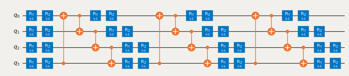
circuit = efficient_su2(num_qubits=4, entanglement="circular")
circuit.assign_parameters([0.4] * len(circuit.parameters), inplace=True)
circuit.draw("mpl", scale=0.8)
ระบุ observable
from qiskit.quantum_info import SparsePauliOp

observable = SparsePauliOp(["ZZII", "IZZI", "-IIZZ", "XIXI", "ZIZZ", "IXIX"])
ขั้นตอนที่ 2: ปรับแต่ง
ระบุ Backend
สามารถใช้ fake backend หรือ hardware backend จาก Qiskit Runtime ก็ได้
from qiskit_ibm_runtime.fake_provider import FakeManilaV2

backend = FakeManilaV2()
Transpile Circuit, ดู swap และสังเกตความลึก
เราเลือก layout ที่ต้องการ swap สองครั้งเพื่อรัน Gate ระหว่าง Qubit 3 กับ 0 และ swap อีกสองครั้งเพื่อคืน Qubit กลับสู่ตำแหน่งเดิม
from qiskit.transpiler import generate_preset_pass_manager

pass_manager = generate_preset_pass_manager(
    optimization_level=1, backend=backend, initial_layout=[0, 1, 2, 3]
)

transpiled_qc = pass_manager.run(circuit)
print(f"Transpiled circuit depth: {transpiled_qc.depth(lambda x: len(x.qubits) >= 2)}")
Transpiled circuit depth: 30
transpiled_qc.draw("mpl", scale=0.4, idle_wires=False, fold=-1)

แทนที่ Gate ที่อยู่ห่างกันด้วย TwoQubitQPDGate โดยระบุ index
cut_gates จะแทนที่ Gate ใน index ที่ระบุด้วย TwoQubitQPDGate และยังคืนรายการของ QPDBasis instance ด้วย — หนึ่งรายการต่อการแตก Gate แต่ละตัว
from qiskit_addon_cutting import cut_gates

# Find the indices of the distant gates
cut_indices = [
    i
    for i, instruction in enumerate(circuit.data)
    if {circuit.find_bit(q)[0] for q in instruction.qubits} == {0, 3}
]

# Decompose distant CNOTs into TwoQubitQPDGate instances
qpd_circuit, bases = cut_gates(circuit, cut_indices)

qpd_circuit.draw("mpl", scale=0.8)

สร้าง subexperiments สำหรับรันบน Backend
generate_cutting_experiments รับ Circuit ที่มี TwoQubitQPDGate และ observables ในรูปแบบ PauliList
เพื่อจำลอง expectation value ของ Circuit ขนาดเต็ม จะมีการสร้าง subexperiments จำนวนมากจาก joint quasiprobability distribution ของ Gate ที่ถูกแตก แล้วนำไปรันบน Backend หนึ่งตัวหรือมากกว่า จำนวนตัวอย่างที่สุ่มจาก distribution ควบคุมด้วย num_samples และจะได้ค่า coefficient รวมหนึ่งค่าต่อตัวอย่างที่ไม่ซ้ำกัน สำหรับข้อมูลเพิ่มเติมเกี่ยวกับการคำนวณ coefficient ดูที่ เนื้อหาอธิบาย
หมายเหตุ: อาร์กิวเมนต์ observables ของ generate_cutting_experiments มีประเภทเป็น PauliList ค่า coefficient และ phase ของ observable term จะถูกละเว้นระหว่างการแตกปัญหาและการรัน subexperiments แต่สามารถนำกลับมาใช้ได้ในขั้นตอนการสร้าง expectation value ขึ้นใหม่
import numpy as np
from qiskit_addon_cutting import generate_cutting_experiments

# Generate the subexperiments and sampling coefficients
subexperiments, coefficients = generate_cutting_experiments(
    circuits=qpd_circuit, observables=observable.paulis, num_samples=np.inf
)
คำนวณ sampling overhead สำหรับการตัดที่เลือก
ในที่นี้เราตัด CNOT gate สามตัว ส่งผลให้มี sampling overhead เป็น
สำหรับข้อมูลเพิ่มเติมเกี่ยวกับ sampling overhead ที่เกิดจากการตัด Circuit ดูที่ เนื้อหาอธิบาย
print(f"Sampling overhead: {np.prod([basis.overhead for basis in bases])}")
Sampling overhead: 729.0
แสดงให้เห็นว่า QPD subexperiments จะตื้นลงหลังจากตัด Gate ที่อยู่ห่างกัน
นี่คือตัวอย่าง subexperiment หนึ่งที่เลือกมาแบบไม่เจาะจงจากบรรดา subexperiment ที่สร้างจาก QPD Circuit ความลึกลดลงมากกว่าครึ่ง ต้องสร้างและประเมิน subexperiment เชิงความน่าจะเป็นเหล่านี้จำนวนมาก เพื่อสร้าง expectation value ของ Circuit ที่ลึกกว่าขึ้นใหม่
# Transpile the decomposed circuit to the same layout
transpiled_qpd_circuit = pass_manager.run(subexperiments[100])

print(
    f"Original circuit depth after transpile: {transpiled_qc.depth(lambda x: len(x.qubits) >= 2)}"
)
print(
    f"QPD subexperiment depth after transpile: {transpiled_qpd_circuit.depth(lambda x: len(x.qubits) >= 2)}"
)
transpiled_qpd_circuit.draw("mpl", scale=0.8, idle_wires=False, fold=-1)
Original circuit depth after transpile: 30
QPD subexperiment depth after transpile: 7

เตรียม subexperiments สำหรับ Backend
# Transpile the subeperiments to the backend's instruction set architecture (ISA)
isa_subexperiments = pass_manager.run(subexperiments)
ขั้นตอนที่ 3: รัน
รัน subexperiments โดยใช้ Qiskit Runtime Sampler primitive
from qiskit_ibm_runtime import SamplerV2

# Set up the Qiskit Runtime Sampler primitive.  For a fake backend, this will use a local simulator.
sampler = SamplerV2(backend)

# Submit the subexperiments
job = sampler.run(isa_subexperiments)
# Retrieve the results
results = job.result()
ขั้นตอนที่ 4: ประมวลผลหลังการรัน
สร้าง expectation value ขึ้นใหม่
สร้าง expectation value ใหม่สำหรับแต่ละ observable term แล้วนำมารวมกันเพื่อสร้าง expectation value ของ observable ต้นฉบับ
from qiskit_addon_cutting import reconstruct_expectation_values

reconstructed_expval_terms = reconstruct_expectation_values(
    results,
    coefficients,
    observable.paulis,
)
# Reconstruct final expectation value
reconstructed_expval = np.dot(reconstructed_expval_terms, observable.coeffs)
เปรียบเทียบ expectation value ที่สร้างขึ้นใหม่กับค่าที่แน่นอนจาก Circuit และ observable ต้นฉบับ
from qiskit_aer.primitives import EstimatorV2

estimator = EstimatorV2()
exact_expval = estimator.run([(circuit, observable)]).result()[0].data.evs
print(f"Reconstructed expectation value: {np.real(np.round(reconstructed_expval, 8))}")
print(f"Exact expectation value: {np.round(exact_expval, 8)}")
print(f"Error in estimation: {np.real(np.round(reconstructed_expval-exact_expval, 8))}")
print(
    f"Relative error in estimation: {np.real(np.round((reconstructed_expval-exact_expval) / exact_expval, 8))}"
)
Reconstructed expectation value: 0.44018555
Exact expectation value: 0.50497603
Error in estimation: -0.06479049
Relative error in estimation: -0.12830408