การปรับปรุงการประมาณพลังงานของ Chemistry Hamiltonian ด้วย SQD

ใน tutorial นี้ เราจะสร้าง Qiskit pattern ที่แสดงวิธีประมวลผลตัวอย่างควอนตัมที่มีสัญญาณรบกวนเพื่อหาค่าประมาณของ ground state ของ chemistry Hamiltonian: โมเลกุล $N_2$ ที่สภาวะสมดุลในชุดฐาน 6-31G เราจะใช้ แนวทาง sample-based quantum diagonalization เพื่อประมวลผลตัวอย่างจาก quantum circuit ansatz ขนาด 36-qubit (ในที่นี้คือ LUCJ circuit) และเพื่อรับมือกับผลกระทบจากสัญญาณรบกวนของควอนตัม จะใช้เทคนิค configuration recovery

pattern นี้แบ่งออกเป็นสี่ขั้นตอน:

ขั้นตอนที่ 1: แปลงปัญหาเป็นปัญหาควอนตัม
- สร้าง ansatz สำหรับประมาณ ground state
ขั้นตอนที่ 2: ปรับแต่งปัญหา
- Transpile ansatz ให้เหมาะกับ Backend
ขั้นตอนที่ 3: ทำการทดลอง
- สุ่มตัวอย่างจาก ansatz โดยใช้ primitive Sampler
ขั้นตอนที่ 4: ประมวลผลผลลัพธ์
- Self-consistent configuration recovery loop
  - ประมวลผลชุด bitstring ตัวอย่างทั้งหมด โดยใช้ความรู้เบื้องต้นเกี่ยวกับจำนวนอนุภาคและค่าเฉลี่ยของ orbital occupancy ที่คำนวณได้จากรอบการวนซ้ำล่าสุด
  - สร้างชุดย่อยของตัวอย่างแบบ probabilistic จาก bitstring ที่ผ่านการ recover แล้ว
  - Project และ diagonalize molecular Hamiltonian บน subspace ของแต่ละตัวอย่าง
  - บันทึกค่าพลังงาน ground state ต่ำสุดที่พบในทุก batch และอัปเดตค่าเฉลี่ย orbital occupancy

สำหรับตัวอย่างนี้ Hamiltonian ของอิเล็กตรอนที่มีปฏิสัมพันธ์กันมีรูปแบบทั่วไปดังนี้:

\hat{H} = \sum_{ \substack{pr\\\sigma} } h_{pr} \, \hat{a}^\dagger_{p\sigma} \hat{a}_{r\sigma} + \sum_{ \substack{prqs\\\sigma\tau} } \frac{(pr|qs)}{2} \, \hat{a}^\dagger_{p\sigma} \hat{a}^\dagger_{q\tau} \hat{a}_{s\tau} \hat{a}_{r\sigma}

$\hat{a}^\dagger_{p\sigma}$ / $\hat{a}_{p\sigma}$ คือ fermionic creation/annihilation operators ที่สัมพันธ์กับองค์ประกอบชุดฐานลำดับที่ $p$ และ spin $\sigma$ ส่วน $h_{pr}$ และ $(pr|qs)$ คือ one- และ two-body electronic integrals

workflow ของ SQD พร้อมกับ self-consistent configuration recovery แสดงไว้ในแผนภาพต่อไปนี้

SQD diagram

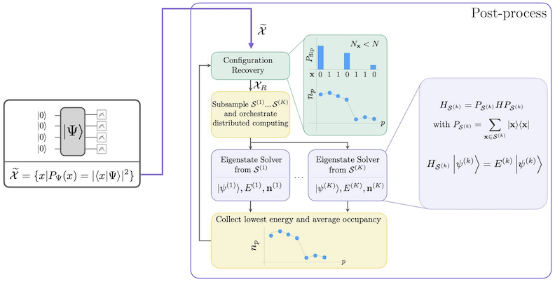
SQD ทำงานได้ดีเมื่อ eigenstate เป้าหมายมีความ sparse: wave function มีค่าไม่เป็นศูนย์อยู่ในชุดของ basis states $\mathcal{S} = \{|x\rangle \}$ ที่ขนาดไม่เพิ่มขึ้นแบบ exponential ตามขนาดของปัญหา ในกรณีนี้ การ diagonalization ของ Hamiltonian ที่ project ลงบน subspace ที่นิยามโดย $\mathcal{S}$ :

H_\mathcal{S} = P_\mathcal{S} H P_\mathcal{S} \textrm{ with } P_\mathcal{S} = \sum_{x \in \mathcal{S}} |x \rangle \langle x |;

จะให้ค่าประมาณที่ดีของ eigenstate เป้าหมาย บทบาทของอุปกรณ์ควอนตัมคือการผลิตตัวอย่างของสมาชิกใน $\mathcal{S}$ เท่านั้น ก่อนอื่น quantum circuit จะเตรียม state $|\Psi\rangle$ ในอุปกรณ์ควอนตัม โดยใช้ Jordan-Wigner encoding ดังนั้น สมาชิกของ computational basis จึงแทน Fock states (electronic configurations/determinants) Circuit จะถูก sample ใน computational basis ให้ได้ชุดของ noisy configurations $\tilde{\mathcal{X}}$ ซึ่งแทนด้วย bitstring จากนั้นชุด $\tilde{\mathcal{X}}$ จะถูกส่งไปยัง classical post-processing block ที่ใช้ เทคนิค self-consistent configuration recovery ใน framework ของ SQD บทบาทของอุปกรณ์ควอนตัมคือการผลิต probability distribution

ขั้นตอนที่ 1: แปลงปัญหาเป็น quantum circuit

ใน tutorial นี้ เราจะประมาณพลังงาน ground state ของโมเลกุล $N_2$ ก่อนอื่นจะระบุคุณสมบัติของโมเลกุล จากนั้นจะสร้าง local unitary cluster Jastrow (LUCJ) ansatz (quantum circuit) เพื่อสุ่มตัวอย่างจากคอมพิวเตอร์ควอนตัมสำหรับการประมาณพลังงาน ground state

ก่อนอื่น เราจะระบุโมเลกุลและคุณสมบัติของมัน

# Added by doQumentation — required packages for this notebook
!pip install -q ffsim matplotlib numpy pyscf qiskit qiskit-addon-sqd qiskit-ibm-runtime

import warnings

warnings.filterwarnings("ignore")

import pyscf
import pyscf.cc
import pyscf.mcscf

# Specify molecule properties
open_shell = False
spin_sq = 0

# Build N2 molecule
mol = pyscf.gto.Mole()
mol.build(
    atom=[["N", (0, 0, 0)], ["N", (1.0, 0, 0)]],
    basis="6-31g",
    symmetry="Dooh",
)

# Define active space
n_frozen = 2
active_space = range(n_frozen, mol.nao_nr())

# Get molecular integrals
scf = pyscf.scf.RHF(mol).run()
num_orbitals = len(active_space)
n_electrons = int(sum(scf.mo_occ[active_space]))
num_elec_a = (n_electrons + mol.spin) // 2
num_elec_b = (n_electrons - mol.spin) // 2
cas = pyscf.mcscf.CASCI(scf, num_orbitals, (num_elec_a, num_elec_b))
mo = cas.sort_mo(active_space, base=0)
hcore, nuclear_repulsion_energy = cas.get_h1cas(mo)
eri = pyscf.ao2mo.restore(1, cas.get_h2cas(mo), num_orbitals)

# Compute exact energy
exact_energy = cas.run().e_tot

converged SCF energy = -108.835236570775
CASCI E = -109.046671778080  E(CI) = -32.8155692383188  S^2 = 0.0000000

ต่อไปเราจะสร้าง ansatz โดย LUCJ ansatz คือ parameterized quantum circuit และเราจะกำหนดค่าเริ่มต้นด้วย amplitude t2 และ t1 ที่ได้จากการคำนวณ CCSD

# Get CCSD t2 amplitudes for initializing the ansatz
ccsd = pyscf.cc.CCSD(scf, frozen=[i for i in range(mol.nao_nr()) if i not in active_space]).run()
t1 = ccsd.t1
t2 = ccsd.t2

E(CCSD) = -109.0398256929734  E_corr = -0.2045891221988311

เราจะใช้แพ็กเกจ ffsim เพื่อสร้างและกำหนดค่าเริ่มต้น ansatz ด้วย amplitude t2 และ t1 ที่คำนวณไว้ข้างต้น เนื่องจากโมเลกุลของเรามี closed-shell Hartree-Fock state จึงจะใช้รูปแบบ spin-balanced ของ UCJ ansatz คือ UCJOpSpinBalanced

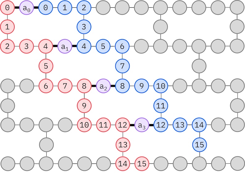
เนื่องจาก IBM hardware เป้าหมายมี heavy-hex topology เราจะใช้ zig-zag pattern สำหรับการเชื่อมต่อ qubit ในรูปแบบนี้ orbital (ที่แทนด้วย qubit) ที่มี spin เดียวกันจะเชื่อมต่อกันแบบ line topology (วงกลมสีแดงและน้ำเงิน) โดยแต่ละเส้นจะมีรูปร่างซิกแซกเนื่องจากการเชื่อมต่อแบบ heavy-hex ของ hardware เป้าหมาย และด้วย heavy-hex topology เช่นกัน orbital ที่ต่าง spin จะมีการเชื่อมต่อกันทุกๆ orbital ที่ 4 (0, 4, 8 เป็นต้น) (วงกลมสีม่วง)

lucj_ansatz

import ffsim
from qiskit import QuantumCircuit, QuantumRegister

n_reps = 1
alpha_alpha_indices = [(p, p + 1) for p in range(num_orbitals - 1)]
alpha_beta_indices = [(p, p) for p in range(0, num_orbitals, 4)]

ucj_op = ffsim.UCJOpSpinBalanced.from_t_amplitudes(
    t2=t2,
    t1=t1,
    n_reps=n_reps,
    interaction_pairs=(alpha_alpha_indices, alpha_beta_indices),
)

nelec = (num_elec_a, num_elec_b)

# create an empty quantum circuit
qubits = QuantumRegister(2 * num_orbitals, name="q")
circuit = QuantumCircuit(qubits)

# prepare Hartree-Fock state as the reference state and append it to the quantum circuit
circuit.append(ffsim.qiskit.PrepareHartreeFockJW(num_orbitals, nelec), qubits)

# apply the UCJ operator to the reference state
circuit.append(ffsim.qiskit.UCJOpSpinBalancedJW(ucj_op), qubits)
circuit.measure_all()

ขั้นตอนที่ 2: ปรับแต่งปัญหา

ต่อไป เราจะปรับแต่ง Circuit ให้เหมาะกับ hardware เป้าหมาย เราต้องเลือกอุปกรณ์ hardware ก่อนที่จะปรับแต่ง Circuit เราจะใช้ fake 127-qubit Backend จาก qiskit_ibm_runtime เพื่อจำลองอุปกรณ์จริง ถ้าต้องการรันบน QPU จริง เพียงแค่เปลี่ยน fake Backend เป็น Backend จริง ดูข้อมูลเพิ่มเติมได้ที่ Qiskit IBM Runtime docs

from qiskit_ibm_runtime.fake_provider import FakeSherbrooke

backend = FakeSherbrooke()

ต่อไป เราแนะนำขั้นตอนต่อไปนี้เพื่อปรับแต่ง ansatz ให้เข้ากันได้กับ hardware

เลือก physical qubit (initial_layout) จาก hardware เป้าหมายที่เป็นไปตาม zig-zag pattern ที่อธิบายข้างต้น การวาง qubit ตามรูปแบบนี้จะทำให้ได้ Circuit ที่เข้ากันได้กับ hardware อย่างมีประสิทธิภาพโดยใช้ Gate น้อยลง
สร้าง staged pass manager โดยใช้ฟังก์ชัน generate_preset_pass_manager จาก Qiskit พร้อมกับ backend และ initial_layout ที่เลือก
กำหนด pre_init stage ของ staged pass manager เป็น ffsim.qiskit.PRE_INIT ซึ่งรวม Transpiler passes ของ Qiskit ที่ decompose Gate เป็น orbital rotation แล้วรวม orbital rotation เข้าด้วยกัน ส่งผลให้ Circuit สุดท้ายมี Gate น้อยลง
รัน pass manager บน Circuit ของเรา

from qiskit.transpiler.preset_passmanagers import generate_preset_pass_manager

spin_a_layout = [0, 14, 18, 19, 20, 33, 39, 40, 41, 53, 60, 61, 62, 72, 81, 82]
spin_b_layout = [2, 3, 4, 15, 22, 23, 24, 34, 43, 44, 45, 54, 64, 65, 66, 73]
initial_layout = spin_a_layout + spin_b_layout

pass_manager = generate_preset_pass_manager(
    optimization_level=3, backend=backend, initial_layout=initial_layout
)

# without PRE_INIT passes
isa_circuit = pass_manager.run(circuit)
print(f"Gate counts (w/o pre-init passes): {isa_circuit.count_ops()}")

# with PRE_INIT passes
# We will use the circuit generated by this pass manager for hardware execution
pass_manager.pre_init = ffsim.qiskit.PRE_INIT
isa_circuit = pass_manager.run(circuit)
print(f"Gate counts (w/ pre-init passes): {isa_circuit.count_ops()}")

Gate counts (w/o pre-init passes): OrderedDict({'rz': 4420, 'sx': 3432, 'ecr': 1366, 'x': 239, 'measure': 32, 'barrier': 1})
Gate counts (w/ pre-init passes): OrderedDict({'rz': 2460, 'sx': 2156, 'ecr': 730, 'x': 71, 'measure': 32, 'barrier': 1})

Step 3: Execute experiments

หลังจาก optimize วงจรสำหรับการรันบนฮาร์ดแวร์แล้ว เราก็พร้อมรันบนฮาร์ดแวร์จริงและเก็บ sample สำหรับการประมาณพลังงาน ground state ได้เลย เนื่องจากเรามีวงจรเดียว เราจะใช้ Job execution mode ของ Qiskit Runtime และรันวงจรของเรา

หมายเหตุ: เราได้คอมเมนต์โค้ดสำหรับรันวงจรบน QPU ไว้เป็นข้อมูลอ้างอิงสำหรับผู้ใช้ แทนที่จะรันบนฮาร์ดแวร์จริงในบทแนะนำนี้ เราจะสร้าง random sample จากการกระจาย uniform แทน

import numpy as np
from qiskit_addon_sqd.counts import generate_bit_array_uniform

# from qiskit_ibm_runtime import SamplerV2 as Sampler

# sampler = Sampler(mode=backend)
# job = sampler.run([isa_circuit], shots=10_000)
# primitive_result = job.result()
# pub_result = primitive_result[0]
# bit_array = pub_result.data.meas

rng = np.random.default_rng(24)
bit_array = generate_bit_array_uniform(10_000, num_orbitals * 2, rand_seed=rng)

Step 4: Post-process results

ตอนนี้เราจะรัน SQD algorithm โดยใช้ฟังก์ชัน diagonalize_fermionic_hamiltonian ดูที่ API documentation สำหรับคำอธิบาย argument ของฟังก์ชันนี้

solver ที่รวมอยู่ใน SQD addon ใช้ implementation ของ selected CI จาก PySCF โดยเฉพาะคือ pyscf.fci.selected_ci.kernel_fixed_space ตัวอย่างด้านล่างยังแสดงวิธีส่ง keyword argument ไปยังฟังก์ชันนั้นผ่าน solver ที่รวมมาด้วย ที่นี่เราส่ง argument max_cycle

from functools import partial

from qiskit_addon_sqd.fermion import SCIResult, diagonalize_fermionic_hamiltonian, solve_sci_batch

# SQD options
energy_tol = 1e-3
occupancies_tol = 1e-3
max_iterations = 5

# Eigenstate solver options
num_batches = 1
samples_per_batch = 300
symmetrize_spin = True
carryover_threshold = 1e-4
max_cycle = 200

# Pass options to the built-in eigensolver. If you just want to use the defaults,
# you can omit this step, in which case you would not specify the sci_solver argument
# in the call to diagonalize_fermionic_hamiltonian below.
sci_solver = partial(solve_sci_batch, spin_sq=0.0, max_cycle=max_cycle)

# List to capture intermediate results
result_history = []

def callback(results: list[SCIResult]):
    result_history.append(results)
    iteration = len(result_history)
    print(f"Iteration {iteration}")
    for i, result in enumerate(results):
        print(f"\tSubsample {i}")
        print(f"\t\tEnergy: {result.energy + nuclear_repulsion_energy}")
        print(f"\t\tSubspace dimension: {np.prod(result.sci_state.amplitudes.shape)}")

result = diagonalize_fermionic_hamiltonian(
    hcore,
    eri,
    bit_array,
    samples_per_batch=samples_per_batch,
    norb=num_orbitals,
    nelec=nelec,
    num_batches=num_batches,
    energy_tol=energy_tol,
    occupancies_tol=occupancies_tol,
    max_iterations=max_iterations,
    sci_solver=sci_solver,
    symmetrize_spin=symmetrize_spin,
    carryover_threshold=carryover_threshold,
    callback=callback,
    seed=rng,
)

Iteration 1
	Subsample 0
		Energy: -105.45358671756313
		Subspace dimension: 5476
Iteration 2
	Subsample 0
		Energy: -107.95172900082163
		Subspace dimension: 249001
Iteration 3
	Subsample 0
		Energy: -108.97460330369815
		Subspace dimension: 339889
Iteration 4
	Subsample 0
		Energy: -109.02739376648793
		Subspace dimension: 440896
Iteration 5
	Subsample 0
		Energy: -109.030972328451
		Subspace dimension: 597529

ตอนนี้เราจะ plot ผลลัพธ์กัน

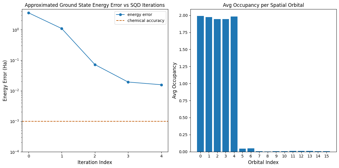
กราฟแรกแสดงให้เห็นว่าหลังจากผ่านไปไม่กี่ iteration เราสามารถประมาณพลังงาน ground state ได้ภายใน ~16 mH (ความแม่นยำทางเคมีโดยทั่วไปยอมรับที่ 1 kcal/mol $\approx$ 1.6 mH) จำไว้ว่า quantum sample ในเดโมนี้เป็นแค่ noise ล้วนๆ signal ที่ได้มาจาก ความรู้เบื้องต้น เกี่ยวกับโครงสร้างอิเล็กทรอนิกส์และ molecular Hamiltonian

กราฟที่สองแสดงค่าเฉลี่ยการครอบครอง (occupancy) ของแต่ละ spatial orbital หลัง iteration สุดท้าย เราจะเห็นว่าทั้งอิเล็กตรอน spin-up และ spin-down ครอบครอง orbital ห้าตัวแรกด้วยความน่าจะเป็นสูงในผลลัพธ์ของเรา

import matplotlib.pyplot as plt

# Data for energies plot
x1 = range(len(result_history))
min_e = [
    min(result, key=lambda res: res.energy).energy + nuclear_repulsion_energy
    for result in result_history
]
e_diff = [abs(e - exact_energy) for e in min_e]
yt1 = [1.0, 1e-1, 1e-2, 1e-3, 1e-4]

# Chemical accuracy (+/- 1 milli-Hartree)
chem_accuracy = 0.001

# Data for avg spatial orbital occupancy
y2 = np.sum(result.orbital_occupancies, axis=0)
x2 = range(len(y2))

fig, axs = plt.subplots(1, 2, figsize=(12, 6))

# Plot energies
axs[0].plot(x1, e_diff, label="energy error", marker="o")
axs[0].set_xticks(x1)
axs[0].set_xticklabels(x1)
axs[0].set_yticks(yt1)
axs[0].set_yticklabels(yt1)
axs[0].set_yscale("log")
axs[0].set_ylim(1e-4)
axs[0].axhline(y=chem_accuracy, color="#BF5700", linestyle="--", label="chemical accuracy")
axs[0].set_title("Approximated Ground State Energy Error vs SQD Iterations")
axs[0].set_xlabel("Iteration Index", fontdict={"fontsize": 12})
axs[0].set_ylabel("Energy Error (Ha)", fontdict={"fontsize": 12})
axs[0].legend()

# Plot orbital occupancy
axs[1].bar(x2, y2, width=0.8)
axs[1].set_xticks(x2)
axs[1].set_xticklabels(x2)
axs[1].set_title("Avg Occupancy per Spatial Orbital")
axs[1].set_xlabel("Orbital Index", fontdict={"fontsize": 12})
axs[1].set_ylabel("Avg Occupancy", fontdict={"fontsize": 12})

print(f"Exact energy: {exact_energy:.5f} Ha")
print(f"SQD energy: {min_e[-1]:.5f} Ha")
print(f"Absolute error: {e_diff[-1]:.5f} Ha")
plt.tight_layout()
plt.show()

Exact energy: -109.04667 Ha
SQD energy: -109.03097 Ha
Absolute error: 0.01570 Ha

Plot output

ขั้นตอนที่ 1: แปลงปัญหาเป็น quantum circuit​

ขั้นตอนที่ 2: ปรับแต่งปัญหา​

Step 3: Execute experiments​

Step 4: Post-process results​

ขั้นตอนที่ 1: แปลงปัญหาเป็น quantum circuit

ขั้นตอนที่ 2: ปรับแต่งปัญหา

Step 3: Execute experiments

Step 4: Post-process results