การปรับปรุงการประมาณพลังงานของโมเดลตาข่าย Fermionic ด้วย SQD
ในบทแนะนำนี้ เราจะสร้าง Qiskit pattern ที่แสดงวิธีการประมวลผลหลัง (post-process) ตัวอย่างควอนตัมที่มีสัญญาณรบกวน เพื่อหาการประมาณสถานะพื้น (ground state) ของ Hamiltonian ตาข่าย Fermionic ที่เรียกว่า single-impurity Anderson model เราจะใช้แนวทาง sample-based quantum diagonalization เพื่อประมวลผลตัวอย่างที่ได้จากชุดสถานะฐาน Krylov ขนาด 16-Qubit ในช่วงเวลาที่เพิ่มขึ้นเรื่อยๆ สถานะเหล่านี้ถูกสร้างบนอุปกรณ์ควอนตัมโดยใช้ Trotterization ของวิวัฒนาการตามเวลา เพื่อรับมือกับผลกระทบของสัญญาณรบกวนควอนตัม จึงใช้เทคนิค configuration recovery แนวทางนี้ได้รับการพิสูจน์ว่าลู่เข้าอย่างมีประสิทธิภาพ เมื่อสถานะเริ่มต้นดีและสถานะพื้นมีความเบาบาง (sparsity)
รูปแบบสามารถอธิบายได้ใน 4 ขั้นตอน:
-
ขั้นตอนที่ 1: แปลงเป็นปัญหาควอนตัม
- สร้างชุดสถานะฐาน Krylov (กล่าวคือ Circuit วิวัฒนาการตามเวลาแบบ Trotterized) ในช่วงเวลาที่เพิ่มขึ้นเรื่อยๆ เพื่อประมาณสถานะพื้น
-
ขั้นตอนที่ 2: ปรับแต่งปัญหา
- Transpile Circuit สำหรับ Backend
-
ขั้นตอนที่ 3: รันการทดลอง
- ดึงตัวอย่าง (sample) จาก circuit โดยใช้ primitive
Sampler
- ดึงตัวอย่าง (sample) จาก circuit โดยใช้ primitive
-
ขั้นตอนที่ 4: ประมวลผลผลลัพธ์
-
ลูป self-consistent configuration recovery
-
ประมวลผลชุดตัวอย่าง bitstring ทั้งหมด โดยใช้ความรู้ล่วงหน้าเกี่ยวกับจำนวนอนุภาคและค่าเฉลี่ยการครอบครอง orbital ที่คำนวณจากการวนซ้ำล่าสุด
-
สร้าง batch ของ subsample จาก bitstring ที่กู้คืนแล้วแบบความน่าจะเป็น
-
โปรเจกต์และ diagonalize Hamiltonian ตาข่าย Fermionic บน subspace แต่ละตัวที่สุ่มมา
-
บันทึกพลังงานสถานะพื้นต่ำสุดที่พบในทุก batch และอัปเดตค่าเฉลี่ยการครอบครอง orbital
-
-
ขั้นตอนที่ 1: แปลงปัญหาเป็น Circuit ควอนตัม
ก่อนอื่น เราจะสร้าง Hamiltonian แบบหนึ่งตัวและสองตัวที่อธิบาย single-impurity Anderson model (SIAM) แบบหนึ่งมิติพร้อม bath sites จำนวน 7 แห่ง (อิเล็กตรอน 8 ตัวใน 8 orbital) โมเดลนี้ใช้สำหรับอธิบายสิ่งเจือปนแม่เหล็ก (magnetic impurities) ที่ฝังอยู่ในโลหะ
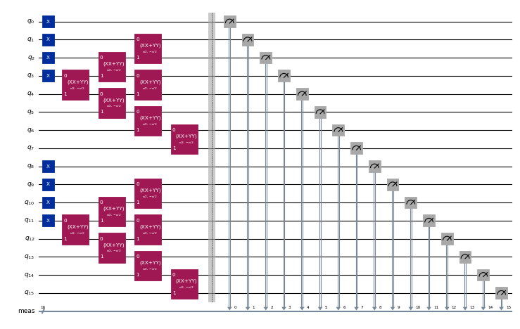
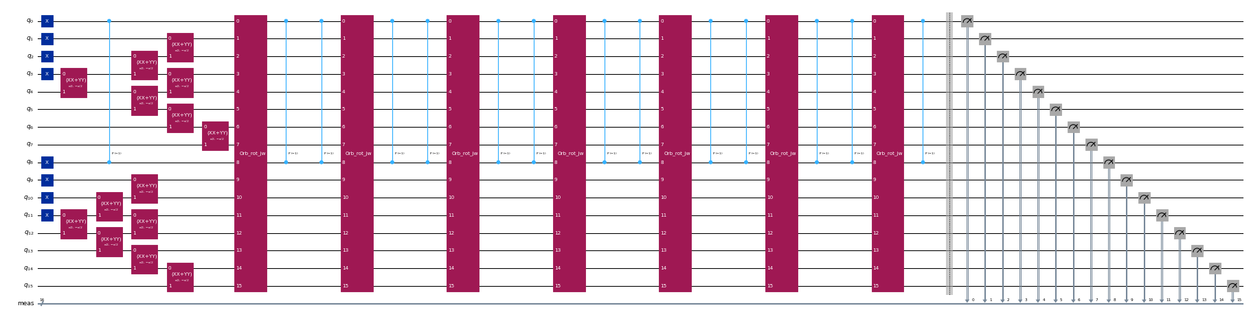
จากนั้นเราจะสร้าง Trotter Circuit ขนาด 16-Qubit ที่ใช้สร้าง quantum Krylov subspace
# Added by doQumentation — installs the packages this notebook needs if they are missing
import importlib.util

_needed = {"ffsim": "ffsim", "matplotlib": "matplotlib", "numpy": "numpy", "qiskit": "qiskit", "qiskit_addon_sqd": "qiskit-addon-sqd", "qiskit_ibm_runtime": "qiskit-ibm-runtime", "scipy": "scipy"}
_missing = [pip for module, pip in _needed.items()
            if importlib.util.find_spec(module) is None]
# One at a time, so a package that fails to install does not block the others
for _pip in _missing:
    %pip install -q {_pip}
if not _missing:
    print("\u2713 All required packages are installed")
import numpy as np

n_bath = 7  # number of bath sites

V = 1  # hybridization amplitude
t = 1  # bath hopping amplitude
U = 10  # Impurity onsite repulsion
eps = -U / 2  # Chemical potential for the impurity

# Place the impurity on the first qubit
impurity_index = 0

# One body matrix elements in the "position" basis
h1e = -t * np.diag(np.ones(n_bath), k=1) - t * np.diag(np.ones(n_bath), k=-1)
h1e[impurity_index, impurity_index + 1] = -V
h1e[impurity_index + 1, impurity_index] = -V
h1e[impurity_index, impurity_index] = eps

# Two body matrix elements in the "position" basis
h2e = np.zeros((n_bath + 1, n_bath + 1, n_bath + 1, n_bath + 1))
h2e[impurity_index, impurity_index, impurity_index, impurity_index] = U
ต่อไป เราจะสร้าง quantum Krylov subspace ด้วยชุด Circuit ควอนตัมแบบ Trotterized เราจะสร้าง helper สำหรับสร้างสถานะเริ่มต้น (reference) รวมถึงวิวัฒนาการตามเวลาสำหรับส่วนหนึ่งตัวและสองตัวของ Hamiltonian สำหรับคำอธิบายโดยละเอียดเพิ่มเติมเกี่ยวกับโมเดลนี้และวิธีออกแบบ Circuit โปรดดู บทความ
import ffsim
import scipy
from qiskit import QuantumCircuit, QuantumRegister
from qiskit.circuit.library import CPhaseGate, XGate, XXPlusYYGate

n_modes = n_bath + 1
nelec = (n_modes // 2, n_modes // 2)

dt = 0.2
Utar = scipy.linalg.expm(-1j * dt * h1e)

# The reference state
def initial_state(q_circuit, norb, nocc):
    """Prepare an initial state."""
    for i in range(nocc):
        q_circuit.append(XGate(), [i])
        q_circuit.append(XGate(), [norb + i])
    rot = XXPlusYYGate(np.pi / 2, -np.pi / 2)

    for i in range(3):
        for j in range(nocc - i - 1, nocc + i, 2):
            q_circuit.append(rot, [j, j + 1])
            q_circuit.append(rot, [norb + j, norb + j + 1])
    q_circuit.append(rot, [j + 1, j + 2])
    q_circuit.append(rot, [norb + j + 1, norb + j + 2])

# The one-body time evolution
free_fermion_evolution = ffsim.qiskit.OrbitalRotationJW(n_modes, Utar)

# The two-body time evolution
def append_diagonal_evolution(dt, U, impurity_qubit, num_orb, q_circuit):
    """Append two-body time evolution to a quantum circuit."""
    if U != 0:
        q_circuit.append(
            CPhaseGate(-dt / 2 * U),
            [impurity_qubit, impurity_qubit + num_orb],
        )
สร้างสถานะที่วิวัฒนาการตามเวลาจำนวน d สถานะที่กำหนด quantum Krylov subspace ที่นี่เราเลือก d=8 ข้อผิดพลาดจากการสุ่มตัวอย่างสถานะฐาน Krylov จะลู่เข้าเมื่อ d เพิ่มขึ้น โปรดทราบว่าลักษณะเฉพาะของปัญหานี้อนุญาตให้คอมไพล์วิวัฒนาการหนึ่งตัวได้อย่างมีประสิทธิภาพโดยใช้ OrbitalRotationJW อย่างไรก็ตาม โดยทั่วไปแล้ว สามารถใช้ PauliEvolutionGate ของ Qiskit เพื่อสร้างวิวัฒนาการตามเวลาแบบ Trotterized ของ Hamiltonian ทั้งหมดได้
# Generate the initial state
qubits = QuantumRegister(2 * n_modes, name="q")
init_state = QuantumCircuit(qubits)
initial_state(init_state, n_modes, n_modes // 2)
init_state.draw("mpl", scale=0.4, fold=-1)

d = 8  # Number of Krylov basis states
circuits = []
for i in range(d):
    circ = init_state.copy()
    circuits.append(circ)
    for _ in range(i):
        append_diagonal_evolution(dt, U, impurity_index, n_modes, circ)
        circ.append(free_fermion_evolution, qubits)
        append_diagonal_evolution(dt, U, impurity_index, n_modes, circ)
    circ.measure_all()
circuits[0].draw("mpl", scale=0.4, fold=-1)
circuits[-1].draw("mpl", scale=0.4, fold=-1)
ขั้นตอนที่ 2: ปรับแต่งปัญหา
หลังจากสร้าง Circuit แบบ Trotterized แล้ว เราจะปรับแต่งให้เหมาะสมกับฮาร์ดแวร์เป้าหมาย เราต้องเลือกอุปกรณ์ฮาร์ดแวร์ที่จะใช้ก่อนการปรับแต่ง เราจะใช้ Backend จำลองขนาด 127-Qubit จาก qiskit_ibm_runtime เพื่อจำลองอุปกรณ์จริง หากต้องการรันบน QPU จริง เพียงแทนที่ Backend จำลองด้วย Backend จริง ดูข้อมูลเพิ่มเติมได้ที่ Qiskit IBM Runtime docs
from qiskit_ibm_runtime.fake_provider.backends import FakeSherbrooke

backend = FakeSherbrooke()
ต่อไป เราจะ Transpile Circuit ไปยัง Backend เป้าหมายโดยใช้ Qiskit
from qiskit.transpiler import generate_preset_pass_manager

# The circuit needs to be transpiled to the AerSimulator target
pass_manager = generate_preset_pass_manager(optimization_level=3, backend=backend)
isa_circuits = pass_manager.run(circuits)
ขั้นตอนที่ 3: รันการทดลอง
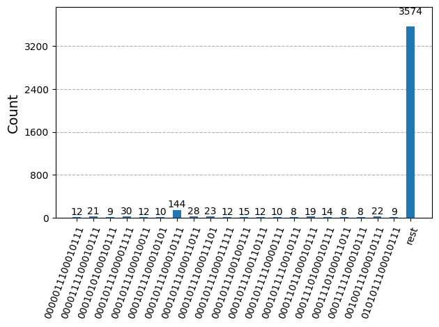
หลังจากปรับแต่ง Circuit สำหรับการรันบนฮาร์ดแวร์แล้ว เราพร้อมรันบนฮาร์ดแวร์เป้าหมายและเก็บตัวอย่างสำหรับการประมาณพลังงานสถานะพื้น ที่นี่เราใช้ SamplerV2 จาก qiskit-ibm-runtime เพื่อจำลองตัวอย่างที่มีสัญญาณรบกวนจาก Backend ibm_sherbrooke จากนั้นเราจะรวม counts จากแต่ละสถานะฐาน Krylov เข้าเป็น counts dictionary เดียวและพล็อต 20 bitstring ที่ถูกสุ่มบ่อยที่สุด
หมายเหตุ: ต้องใช้ Qiskit Aer เพื่อจำลองตัวอย่างจาก Circuit ที่ผ่าน Transpile แล้ว
from qiskit.primitives import BitArray
from qiskit.visualization import plot_histogram
from qiskit_ibm_runtime import SamplerV2 as Sampler

# Sample from the circuits
noisy_sampler = Sampler(backend, options={"simulator": {"seed_simulator": 24}})
job = noisy_sampler.run(isa_circuits, shots=500)

# Combine the counts from the individual Trotter circuits
bit_array = BitArray.concatenate_shots([result.data.meas for result in job.result()])

plot_histogram(bit_array.get_counts(), number_to_keep=20)
ขั้นตอนที่ 4: ประมวลผลผลลัพธ์
ตอนนี้ เราจะรันอัลกอริทึม SQD โดยใช้ฟังก์ชัน diagonalize_fermionic_hamiltonian ดู เอกสาร API สำหรับคำอธิบายของอาร์กิวเมนต์ของฟังก์ชันนี้
from qiskit_addon_sqd.fermion import SCIResult, diagonalize_fermionic_hamiltonian

# List to capture intermediate results
result_history = []

def callback(results: list[SCIResult]):
    result_history.append(results)
    iteration = len(result_history)
    print(f"Iteration {iteration}")
    for i, result in enumerate(results):
        print(f"\tSubsample {i}")
        print(f"\t\tEnergy: {result.energy}")
        print(f"\t\tSubspace dimension: {np.prod(result.sci_state.amplitudes.shape)}")

rng = np.random.default_rng(24)
result = diagonalize_fermionic_hamiltonian(
    h1e,
    h2e,
    bit_array,
    samples_per_batch=300,
    norb=n_modes,
    nelec=nelec,
    num_batches=3,
    max_iterations=10,
    symmetrize_spin=True,
    callback=callback,
    seed=rng,
)
Iteration 1
	Subsample 0
		Energy: -13.257128325607997
		Subspace dimension: 3969
	Subsample 1
		Energy: -13.257128325607997
		Subspace dimension: 3969
	Subsample 2
		Energy: -13.257128325607997
		Subspace dimension: 3969
Iteration 2
	Subsample 0
		Energy: -13.319666127542039
		Subspace dimension: 4096
	Subsample 1
		Energy: -13.420534292304595
		Subspace dimension: 4624
	Subsample 2
		Energy: -9.136171594591085
		Subspace dimension: 4624
Iteration 3
	Subsample 0
		Energy: -13.422491814612833
		Subspace dimension: 4900
	Subsample 1
		Energy: -13.422491814612833
		Subspace dimension: 4900
	Subsample 2
		Energy: -13.422491814612833
		Subspace dimension: 4900
Iteration 4
	Subsample 0
		Energy: -13.422491814612833
		Subspace dimension: 4900
	Subsample 1
		Energy: -13.422491814612833
		Subspace dimension: 4900
	Subsample 2
		Energy: -13.422491814612833
		Subspace dimension: 4900
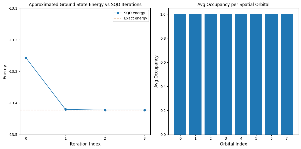
ตอนนี้ เราพล็อตผลลัพธ์ กราฟแรกแสดงให้เห็นว่าหลังจากวนซ้ำไม่กี่ครั้ง เราได้ค่าพลังงานสถานะพื้นที่แม่นตรง (exact)
ตัวอย่างนี้มีขนาดเล็กพอที่เราสามารถสำรวจ Hilbert space เต็มรูปแบบได้ ดังที่เห็นในคำสั่ง print ข้างต้น จำไว้ว่า Hilbert space เต็มรูปแบบมีมิติเท่ากับ (num_orbitals choose nelec_a) * (num_orbitals choose nelec_b) สำหรับปัญหานี้: (8 choose 4)**2 = 4900 มิติของ subspace เพิ่มขึ้นเนื่องจาก configuration recovery ที่ดีขึ้น และยังเนื่องจากอัลกอริทึม SQD นำ configuration ที่สำคัญจากการวนซ้ำหนึ่งไปยังครั้งถัดไป เมื่อถึงการวนซ้ำครั้งสุดท้าย เราทำการ diagonalize ใน Hilbert space ทั้งหมด
กราฟที่สองแสดงการครอบครองเฉลี่ยของ spatial orbital แต่ละตัว จากผลเฉลยของทุก batch เราเห็นว่าด้วยความน่าจะเป็นสูง แต่ละ orbital มีอิเล็กตรอนหนึ่งตัว
import matplotlib.pyplot as plt

exact_energy = -13.422491814605827
min_es = [min(result, key=lambda res: res.energy).energy for result in result_history]
min_id, min_e = min(enumerate(min_es), key=lambda x: x[1])

# Data for energies plot
x1 = range(len(result_history))
yt1 = list(np.arange(-13.5, -13.1, 0.1))
ytl = [f"{i:.1f}" for i in yt1]

# Data for avg spatial orbital occupancy
y2 = np.sum(result.orbital_occupancies, axis=0)
x2 = range(len(y2))

fig, axs = plt.subplots(1, 2, figsize=(12, 6))

# Plot energies
axs[0].plot(x1, min_es, label="SQD energy", marker="o")
axs[0].set_xticks(x1)
axs[0].set_xticklabels(x1)
axs[0].set_yticks(yt1)
axs[0].set_yticklabels(ytl)
axs[0].axhline(y=exact_energy, color="#BF5700", linestyle="--", label="Exact energy")
axs[0].set_title("Approximated Ground State Energy vs SQD Iterations")
axs[0].set_xlabel("Iteration Index", fontdict={"fontsize": 12})
axs[0].set_ylabel("Energy", fontdict={"fontsize": 12})
axs[0].legend()

# Plot orbital occupancy
axs[1].bar(x2, y2, width=0.8)
axs[1].set_xticks(x2)
axs[1].set_xticklabels(x2)
axs[1].set_title("Avg Occupancy per Spatial Orbital")
axs[1].set_xlabel("Orbital Index", fontdict={"fontsize": 12})
axs[1].set_ylabel("Avg Occupancy", fontdict={"fontsize": 12})

print(f"Exact energy: {exact_energy:.5f}")
print(f"SQD energy: {min_e:.5f}")
print(f"Absolute error: {abs(min_e - exact_energy):.5f}")
plt.tight_layout()
plt.show()
Exact energy: -13.42249
SQD energy: -13.42249
Absolute error: 0.00000