การตัด Gate เพื่อลดความกว้างของ Circuit

ใน notebook นี้ เราจะทำตามขั้นตอนของ Qiskit pattern โดยใช้ circuit cutting เพื่อลดจำนวน Qubit ใน Circuit เราจะตัด Gate เพื่อให้สามารถสร้าง expectation value ของ Circuit สี่ Qubit ขึ้นมาใหม่ได้จากการทดลองสองสอง Qubit เท่านั้น

ขั้นตอนที่เราจะดำเนินการมีดังนี้:

• ขั้นตอนที่ 1: แมปปัญหาไปยัง quantum circuit และ operator:
  • แมป Hamiltonian ลงบน quantum circuit
• ขั้นตอนที่ 2: ปรับให้เหมาะกับฮาร์ดแวร์เป้าหมาย [ใช้ cutting addon]:
  • ตัด Circuit และ observable
  • Transpile subexperiment สำหรับฮาร์ดแวร์
• ขั้นตอนที่ 3: รันบนฮาร์ดแวร์เป้าหมาย:
  • รัน subexperiment ที่ได้จากขั้นตอนที่ 2 โดยใช้ primitive Sampler
• ขั้นตอนที่ 4: ประมวลผลผลลัพธ์ [ใช้ cutting addon]:
  • รวมผลลัพธ์จากขั้นตอนที่ 3 เพื่อสร้าง expectation value ของ observable ที่ต้องการขึ้นมาใหม่

ขั้นตอนที่ 1: แมป

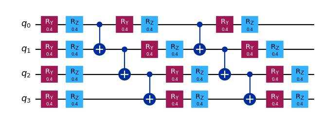
สร้าง Circuit เพื่อตัด

# Added by doQumentation — required packages for this notebook
!pip install -q numpy qiskit qiskit-addon-cutting qiskit-aer qiskit-ibm-runtime

from qiskit.circuit.library import efficient_su2

qc = efficient_su2(4, entanglement="linear", reps=2)
qc.assign_parameters([0.4] * len(qc.parameters), inplace=True)

qc.draw("mpl", scale=0.8)

ระบุ observable

from qiskit.quantum_info import SparsePauliOp

observable = SparsePauliOp(["ZZII", "IZZI", "-IIZZ", "XIXI", "ZIZZ", "IXIX"])

ขั้นตอนที่ 2: ปรับให้เหมาะสม

แยก Circuit และ observable ตามการแบ่งพาร์ติชัน Qubit ที่กำหนด

แต่ละ label ใน partition_labels จะสอดคล้องกับ Qubit ของ circuit ในตำแหน่งเดียวกัน Qubit ที่มี partition label เหมือนกันจะถูกจัดกลุ่มเข้าด้วยกัน และ Gate ที่ไม่ใช่ local ที่ครอบคลุมพาร์ติชันมากกว่าหนึ่งพาร์ติชันจะถูกตัด

หมายเหตุ: argument observables ของ partition_problem มีประเภทเป็น PauliList สัมประสิทธิ์และเฟสของ observable term จะถูกละเว้นระหว่างการ decompose ปัญหาและการรัน subexperiment แต่สามารถนำกลับมาใช้ได้อีกครั้งในระหว่างการสร้าง expectation value ขึ้นมาใหม่

from qiskit_addon_cutting import partition_problem

partitioned_problem = partition_problem(
    circuit=qc, partition_labels="AABB", observables=observable.paulis
)
subcircuits = partitioned_problem.subcircuits
subobservables = partitioned_problem.subobservables
bases = partitioned_problem.bases

แสดงผลปัญหาที่ decompose แล้ว

subobservables

{'A': PauliList(['II', 'ZI', 'ZZ', 'XI', 'ZZ', 'IX']),
 'B': PauliList(['ZZ', 'IZ', 'II', 'XI', 'ZI', 'IX'])}

subcircuits["A"].draw("mpl", scale=0.8)

subcircuits["B"].draw("mpl", scale=0.8)

คำนวณ sampling overhead สำหรับการตัดที่เลือก

ที่นี่เราตัด CNOT Gate สองตัว ส่งผลให้เกิด sampling overhead เป็น $9^2$

สำหรับข้อมูลเพิ่มเติมเกี่ยวกับ sampling overhead ที่เกิดจาก circuit cutting ดูที่ เนื้อหาอธิบาย

import numpy as np

print(f"Sampling overhead: {np.prod([basis.overhead for basis in bases])}")

Sampling overhead: 81.0

สร้าง subexperiment เพื่อรันบน Backend

generate_cutting_experiments รับ argument circuits/observables เป็น dictionary ที่แมป qubit partition label ไปยัง subcircuit/subobservables ที่เกี่ยวข้อง

เพื่อจำลอง expectation value ของ Circuit ขนาดเต็ม จะมีการสร้าง subexperiment จำนวนมากจาก joint quasiprobability distribution ของ Gate ที่ decompose แล้ว จากนั้นรันบน Backend หนึ่งตัวหรือมากกว่า จำนวนตัวอย่างที่นำมาจาก distribution ควบคุมโดย num_samples และจะมีสัมประสิทธิ์รวมหนึ่งตัวสำหรับแต่ละ sample ที่ไม่ซ้ำกัน สำหรับข้อมูลเพิ่มเติมเกี่ยวกับวิธีคำนวณสัมประสิทธิ์ ดูที่ เนื้อหาอธิบาย

from qiskit_addon_cutting import generate_cutting_experiments

subexperiments, coefficients = generate_cutting_experiments(
    circuits=subcircuits, observables=subobservables, num_samples=np.inf
)

เลือก Backend

ที่นี่เราใช้ fake backend ซึ่งจะทำให้ Qiskit Runtime รันในโหมด local (กล่าวคือบน local simulator)

from qiskit_ibm_runtime.fake_provider import FakeManilaV2

backend = FakeManilaV2()

เตรียม subexperiment สำหรับ Backend

เราต้อง Transpile Circuit โดยใช้ Backend ของเราเป็น target ก่อนส่งไปยัง Qiskit Runtime

from qiskit.transpiler import generate_preset_pass_manager

# Transpile the subexperiments to ISA circuits
pass_manager = generate_preset_pass_manager(optimization_level=1, backend=backend)
isa_subexperiments = {
    label: pass_manager.run(partition_subexpts)
    for label, partition_subexpts in subexperiments.items()
}

ขั้นตอนที่ 3: รัน

รัน subexperiment โดยใช้ Qiskit Runtime Sampler primitive

from qiskit_ibm_runtime import SamplerV2, Batch

# Submit each partition's subexperiments to the Qiskit Runtime Sampler
# primitive, in a single batch so that the jobs will run back-to-back.
with Batch(backend=backend) as batch:
    sampler = SamplerV2(mode=batch)
    jobs = {
        label: sampler.run(subsystem_subexpts, shots=2**12)
        for label, subsystem_subexpts in isa_subexperiments.items()
    }

/home/garrison/Qiskit/qiskit-ibm-runtime/qiskit_ibm_runtime/session.py:157: UserWarning: Session is not supported in local testing mode or when using a simulator.
  warnings.warn(

# Retrieve results
results = {label: job.result() for label, job in jobs.items()}

ขั้นตอนที่ 4: ประมวลผลหลังการรัน

สร้าง expectation value ขึ้นมาใหม่

สร้าง expectation value สำหรับแต่ละ observable term ขึ้นมาใหม่ แล้วรวมกันเพื่อสร้าง expectation value ของ observable ต้นฉบับ

from qiskit_addon_cutting import reconstruct_expectation_values

# Get expectation values for each observable term
reconstructed_expval_terms = reconstruct_expectation_values(
    results,
    coefficients,
    subobservables,
)

# Reconstruct final expectation value
reconstructed_expval = np.dot(reconstructed_expval_terms, observable.coeffs)

เปรียบเทียบ expectation value ที่สร้างขึ้นใหม่กับ expectation value ที่แน่นอนจาก Circuit และ observable ต้นฉบับ

from qiskit_aer.primitives import EstimatorV2

estimator = EstimatorV2()
exact_expval = estimator.run([(qc, observable)]).result()[0].data.evs
print(f"Reconstructed expectation value: {np.real(np.round(reconstructed_expval, 8))}")
print(f"Exact expectation value: {np.round(exact_expval, 8)}")
print(f"Error in estimation: {np.real(np.round(reconstructed_expval-exact_expval, 8))}")
print(
    f"Relative error in estimation: {np.real(np.round((reconstructed_expval-exact_expval) / exact_expval, 8))}"
)

Reconstructed expectation value: 0.6991539
Exact expectation value: 0.56254612
Error in estimation: 0.13660778
Relative error in estimation: 0.24283836