การลดความลึกของ Circuit ด้วย Operator Backpropagation
Operator backpropagation เป็นเทคนิคที่ดูดซับ operation จากท้าย quantum circuit เข้าไปใน Pauli operator ซึ่งโดยทั่วไปจะลดความลึกของ Circuit แลกกับจำนวนพจน์ใน operator ที่เพิ่มขึ้น เป้าหมายคือ backpropagate Circuit ให้ได้มากที่สุดโดยไม่ปล่อยให้ operator ใหญ่เกินไป
วิธีหนึ่งที่ช่วยให้ backpropagation เข้าไปใน circuit ได้ลึกขึ้น ในขณะที่ป้องกันไม่ให้ operator ขยายใหญ่เกินไป คือการตัดพจน์ (truncate) ที่มีสัมประสิทธิ์ขนาดเล็กออก แทนที่จะเพิ่มเข้าไปใน operator การตัดพจน์เหล่านี้สามารถลดจำนวน quantum circuit ที่ต้องรันได้ แต่การทำเช่นนี้ก็ทำให้เกิดข้อผิดพลาดบางส่วนในการคำนวณค่าความคาดหวัง (expectation value) สุดท้าย ซึ่งเป็นสัดส่วนกับขนาดของสัมประสิทธิ์ของพจน์ที่ถูกตัดออก ในบทช่วยสอนนี้เราจะนำ Qiskit pattern มาใช้เพื่อจำลองพลศาสตร์เชิงควอนตัมของ Heisenberg spin chain โดยใช้ operator backpropagation:
-
ขั้นตอนที่ 1: แปลงเป็น quantum problem
- แปลง Hamiltonian ที่ผ่านการ time-evolve ให้เป็น quantum circuit
-
ขั้นตอนที่ 2: ปรับปรุง problem
-
แบ่ง Circuit เป็น slice
- Backpropagate slice จาก Circuit ไปยัง Pauli observable
-
รวม slice ที่เหลือเข้าเป็น Circuit เดียว
-
Transpile Circuit สำหรับ Backend
-
-
ขั้นตอนที่ 3: รันการทดลอง
- คำนวณค่าความคาดหวัง (expectation value) โดยใช้ Circuit ที่ลดขนาดแล้วและ observable ที่ขยายออกด้วย StatevectorEstimator เพื่อความง่ายใน notebook นี้
-
ขั้นตอนที่ 4: สร้างผลลัพธ์กลับคืน (reconstruct)
- ไม่มี
หมายเหตุ: Qiskit อธิบาย layers อย่างกว้างๆ ว่าเป็นการแบ่ง Circuit แบบ depth-1 ครอบคลุมทุก Qubit แพ็กเกจนี้ใช้คำว่า slices เพื่ออธิบาย layer ที่มีความลึกได้ตามต้องการ ฟังก์ชัน qiskit_addon_obp.backpropagate ถูกออกแบบให้ backpropagate ทีละ slice ดังนั้นการเลือกวิธีแบ่ง Circuit เป็น slice จึงมีผลอย่างมากต่อประสิทธิภาพของ backpropagation สำหรับแต่ละ problem โดยจะได้เรียนรู้เพิ่มเติมเกี่ยวกับ slices ด้านล่าง
ขั้นตอนที่ 1: แปลงเป็น quantum problem
แปลง time-evolution ของ quantum Heisenberg model เป็นการทดลอง quantum
แพ็กเกจ qiskit_addon_utils มีฟังก์ชันที่ใช้งานซ้ำได้สำหรับหลายวัตถุประสงค์
โมดูล qiskit_addon_utils.problem_generators มีฟังก์ชันสำหรับสร้าง Heisenberg-like Hamiltonians บน connectivity graph ที่กำหนด graph นี้อาจเป็น rustworkx.PyGraph หรือ CouplingMap ก็ได้ ทำให้ใช้งานใน workflow ที่ใช้ Qiskit เป็นศูนย์กลางได้สะดวก
ต่อไปนี้ เราจะสร้าง heavy-hex CouplingMap ก่อน แล้วจึงตัดเอาสาย Qubit แบบ linear chain 10 Qubit ออกมา ทั้งนี้ index ของ reduced_coupling_map ใหม่นี้จะเริ่มจากศูนย์อีกครั้ง
# Added by doQumentation — installs the packages this notebook needs if they are missing
import importlib.util

_needed = {"numpy": "numpy", "qiskit": "qiskit", "qiskit_addon_obp": "qiskit-addon-obp", "qiskit_addon_utils": "qiskit-addon-utils", "qiskit_ibm_runtime": "qiskit-ibm-runtime", "rustworkx": "rustworkx"}
_missing = [pip for module, pip in _needed.items()
            if importlib.util.find_spec(module) is None]
# One at a time, so a package that fails to install does not block the others
for _pip in _missing:
    %pip install -q {_pip}
if not _missing:
    print("\u2713 All required packages are installed")
from qiskit.transpiler import CouplingMap

coupling_map = CouplingMap.from_heavy_hex(3, bidirectional=False)

# Choose a 10-qubit linear chain on this coupling map
reduced_coupling_map = coupling_map.reduce([0, 13, 1, 14, 10, 16, 5, 12, 8, 18])
from rustworkx.visualization import graphviz_draw

graphviz_draw(reduced_coupling_map.graph, method="circo")

ถัดมา เราจะสร้าง Pauli operator สำหรับจำลอง Heisenberg XYZ Hamiltonian
J_{y} \sigma_j^{y} \sigma_{k}^{y} + J_{z} \sigma_j^{z} \sigma_{k}^{z}) + \sum_{j\in V} (h_{x} \sigma_j^{x} + h_{y} \sigma_j^{y} + h_{z} \sigma_j^{z})$$ โดยที่ $G(V,E)$ คือ graph ของ coupling map ที่กำหนดให้ ```python import numpy as np from qiskit_addon_utils.problem_generators import generate_xyz_hamiltonian # Get a qubit operator describing the Heisenberg XYZ model hamiltonian = generate_xyz_hamiltonian( reduced_coupling_map, coupling_constants=(np.pi / 8, np.pi / 4, np.pi / 2), ext_magnetic_field=(np.pi / 3, np.pi / 6, np.pi / 9), ) print(hamiltonian) ``` ```text SparsePauliOp(['IIIIIIIXXI', 'IIIIIIIYYI', 'IIIIIIIZZI', 'IIIIIXXIII', 'IIIIIYYIII', 'IIIIIZZIII', 'IIIXXIIIII', 'IIIYYIIIII', 'IIIZZIIIII', 'IXXIIIIIII', 'IYYIIIIIII', 'IZZIIIIIII', 'IIIIIIIIXX', 'IIIIIIIIYY', 'IIIIIIIIZZ', 'IIIIIIXXII', 'IIIIIIYYII', 'IIIIIIZZII', 'IIIIXXIIII', 'IIIIYYIIII', 'IIIIZZIIII', 'IIXXIIIIII', 'IIYYIIIIII', 'IIZZIIIIII', 'XXIIIIIIII', 'YYIIIIIIII', 'ZZIIIIIIII', 'IIIIIIIIIX', 'IIIIIIIIIY', 'IIIIIIIIIZ', 'IIIIIIIIXI', 'IIIIIIIIYI', 'IIIIIIIIZI', 'IIIIIIIXII', 'IIIIIIIYII', 'IIIIIIIZII', 'IIIIIIXIII', 'IIIIIIYIII', 'IIIIIIZIII', 'IIIIIXIIII', 'IIIIIYIIII', 'IIIIIZIIII', 'IIIIXIIIII', 'IIIIYIIIII', 'IIIIZIIIII', 'IIIXIIIIII', 'IIIYIIIIII', 'IIIZIIIIII', 'IIXIIIIIII', 'IIYIIIIIII', 'IIZIIIIIII', 'IXIIIIIIII', 'IYIIIIIIII', 'IZIIIIIIII', 'XIIIIIIIII', 'YIIIIIIIII', 'ZIIIIIIIII'], coeffs=[0.39269908+0.j, 0.78539816+0.j, 1.57079633+0.j, 0.39269908+0.j, 0.78539816+0.j, 1.57079633+0.j, 0.39269908+0.j, 0.78539816+0.j, 1.57079633+0.j, 0.39269908+0.j, 0.78539816+0.j, 1.57079633+0.j, 0.39269908+0.j, 0.78539816+0.j, 1.57079633+0.j, 0.39269908+0.j, 0.78539816+0.j, 1.57079633+0.j, 0.39269908+0.j, 0.78539816+0.j, 1.57079633+0.j, 0.39269908+0.j, 0.78539816+0.j, 1.57079633+0.j, 0.39269908+0.j, 0.78539816+0.j, 1.57079633+0.j, 1.04719755+0.j, 0.52359878+0.j, 0.34906585+0.j, 1.04719755+0.j, 0.52359878+0.j, 0.34906585+0.j, 1.04719755+0.j, 0.52359878+0.j, 0.34906585+0.j, 1.04719755+0.j, 0.52359878+0.j, 0.34906585+0.j, 1.04719755+0.j, 0.52359878+0.j, 0.34906585+0.j, 1.04719755+0.j, 0.52359878+0.j, 0.34906585+0.j, 1.04719755+0.j, 0.52359878+0.j, 0.34906585+0.j, 1.04719755+0.j, 0.52359878+0.j, 0.34906585+0.j, 1.04719755+0.j, 0.52359878+0.j, 0.34906585+0.j, 1.04719755+0.j, 0.52359878+0.j, 0.34906585+0.j]) ``` จาก qubit operator เราสามารถสร้าง quantum circuit ที่จำลอง time evolution ของมันได้ โมดูล [qiskit_addon_utils.problem_generators](https://qiskit.github.io/qiskit-addon-utils/stubs/qiskit_addon_utils.problem_generators.html) ก็มีฟังก์ชันที่สะดวกสำหรับทำสิ่งนี้เช่นกัน: ```python from qiskit.synthesis import LieTrotter from qiskit_addon_utils.problem_generators import generate_time_evolution_circuit circuit = generate_time_evolution_circuit( hamiltonian, time=0.2, synthesis=LieTrotter(reps=2), ) circuit.draw("mpl", style="iqp", scale=0.6) ``` 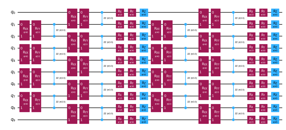 ## ขั้นตอนที่ 2: ปรับปรุง problem \{#step-2-optimize-the-problem} ### สร้าง circuit slice สำหรับ backpropagation \{#create-circuit-slices-to-backpropagate} จำไว้ว่าฟังก์ชัน ``backpropagate`` จะ backpropagate ทีละ slice ดังนั้นการเลือกวิธีแบ่ง slice จึงส่งผลต่อประสิทธิภาพของ backpropagation สำหรับแต่ละ problem ที่นี่ เราจะจัดกลุ่ม Gate ประเภทเดียวกันเข้าด้วยกันเป็น slice โดยใช้ฟังก์ชัน [slice_by_gate_types](https://qiskit.github.io/qiskit-addon-utils/stubs/qiskit_addon_utils.slicing.slice_by_gate_types.html) สำหรับการอภิปรายโดยละเอียดเกี่ยวกับ circuit slicing ดูได้ที่ [how-to guide](https://qiskit.github.io/qiskit-addon-utils/how_tos/create_circuit_slices.html) ของแพ็กเกจ [qiskit-addon-utils](https://qiskit.github.io/qiskit-addon-utils/index.html) ```python from qiskit_addon_utils.slicing import slice_by_gate_types slices = slice_by_gate_types(circuit) print(f"Separated the circuit into {len(slices)} slices.") ``` ```text Separated the circuit into 18 slices. ``` ### กำหนดขีดจำกัดขนาด operator ระหว่าง backpropagation \{#constrain-how-large-the-operator-may-grow-during-backpropagation} ระหว่าง backpropagation จำนวนพจน์ใน operator มักจะเพิ่มขึ้นอย่างรวดเร็วไปถึง $4^N$ โดยที่ $N$ คือจำนวน Qubit ขนาดของ operator สามารถควบคุมได้โดยระบุ kwarg ``operator_budget`` ของฟังก์ชัน ``backpropagate`` ซึ่งรับ instance ของ [OperatorBudget](https://qiskit.github.io/qiskit-addon-obp/stubs/qiskit_addon_obp.utils.simplify.OperatorBudget.html) ที่นี่เราระบุว่า backpropagation ควรหยุดเมื่อจำนวน qubit-wise commuting Pauli group ใน operator เกิน 8 ```python from qiskit_addon_obp.utils.simplify import OperatorBudget op_budget = OperatorBudget(max_qwc_groups=8) ``` ### Backpropagate slice จาก Circuit \{#backpropagate-slices-from-the-circuit} ก่อนอื่น เราจะกำหนด Pauli-Z observable บน Qubit 0 แล้ว backpropagate slice จาก time-evolution circuit จนกว่าพจน์ใน observable จะไม่สามารถรวมให้เป็น 8 qubit-wise commuting Pauli group หรือน้อยกว่าได้อีก ด้านล่างจะเห็นว่าเรา backpropagate ได้ 7 slice แต่ใช้ไปเพียง 6 จาก 8 Pauli group ที่จัดสรรไว้ ซึ่งหมายความว่าการ backpropagate อีก 1 slice จะทำให้จำนวน Pauli group เกิน 8 เราสามารถตรวจสอบสิ่งนี้ได้โดยดูจาก metadata ที่คืนค่ามา ```python from qiskit.quantum_info import SparsePauliOp from qiskit_addon_obp import backpropagate from qiskit_addon_utils.slicing import combine_slices # Specify a single-qubit observable observable = SparsePauliOp("IIIIIIIIIZ") # Backpropagate slices onto the observable bp_obs, remaining_slices, metadata = backpropagate(observable, slices, operator_budget=op_budget) # Recombine the slices remaining after backpropagation bp_circuit = combine_slices(remaining_slices, include_barriers=True) print(f"Backpropagated {metadata.num_backpropagated_slices} slices.") print( f"New observable has {len(bp_obs.paulis)} terms, which can be combined into {len(bp_obs.group_commuting(qubit_wise=True))} groups." ) print( f"Note that backpropagating one more slice would result in {metadata.backpropagation_history[-1].num_paulis[0]} terms " f"across {metadata.backpropagation_history[-1].num_qwc_groups} groups." ) print("The remaining circuit after backpropagation looks as follows:") bp_circuit.draw("mpl", scale=0.6) ``` ```text Backpropagated 7 slices. New observable has 18 terms, which can be combined into 8 groups. Note that backpropagating one more slice would result in 27 terms across 12 groups. The remaining circuit after backpropagation looks as follows: ``` 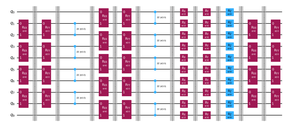 ถัดมา เราจะกำหนด problem เดิมพร้อมข้อจำกัดขนาด output observable เหมือนเดิม แต่คราวนี้เราจะจัดสรร error budget ให้แต่ละ slice โดยใช้ฟังก์ชัน [setup_budet](https://qiskit.github.io/qiskit-addon-obp/stubs/qiskit_addon_obp.utils.truncating.setup_budget.html) Pauli term ที่มีสัมประสิทธิ์ขนาดเล็กจะถูกตัดออกจากแต่ละ slice จนกว่า error budget จะเต็ม และ budget ที่เหลือจะถูกนำไปรวมกับ budget ของ slice ถัดไป เพื่อเปิดใช้งานการตัดแบบนี้ เราต้องตั้งค่า error budget ดังนี้: ```python from qiskit_addon_obp.utils.truncating import setup_budget truncation_error_budget = setup_budget(max_error_per_slice=0.005) ``` สังเกตว่าการจัดสรร `5e-3` error ต่อ slice สำหรับการตัด ทำให้เราลบ slice ออกจาก Circuit ได้อีก 3 slice ขณะที่ยังอยู่ภายใน budget เดิมที่ 8 commuting Pauli group ใน observable โดยค่าเริ่มต้น `backpropagate` จะใช้ L1 norm ของสัมประสิทธิ์ที่ถูกตัดเพื่อจำกัดขอบเขต (bound) ของ total error ที่เกิดจากการตัด สำหรับตัวเลือกอื่นดูได้ที่ [how-to guide on specifying the p_norm](https://qiskit.github.io/qiskit-addon-obp/how_tos/bound_error_using_p_norm.html) ในตัวอย่างนี้ที่เรา backpropagate 10 slice total truncation error ไม่ควรเกิน ``(5e-3 error/slice) * (10 slices) = 5e-2`` สำหรับการอภิปรายเพิ่มเติมเกี่ยวกับการกระจาย error budget ไปยัง slice ต่างๆ ดูได้ที่ [how-to guide นี้](https://qiskit.github.io/qiskit-addon-obp/how_tos/truncate_operator_terms.html) ```python # Run the same experiment but truncate observable terms with small coefficients bp_obs_trunc, remaining_slices_trunc, metadata = backpropagate( observable, slices, operator_budget=op_budget, truncation_error_budget=truncation_error_budget ) # Recombine the slices remaining after backpropagation bp_circuit_trunc = combine_slices(remaining_slices_trunc, include_barriers=True) print(f"Backpropagated {metadata.num_backpropagated_slices} slices.") print( f"New observable has {len(bp_obs_trunc.paulis)} terms, which can be combined into {len(bp_obs_trunc.group_commuting(qubit_wise=True))} groups.\n" f"After truncation, the error in our observable is bounded by {metadata.accumulated_error(0):.3e}" ) print( f"Note that backpropagating one more slice would result in {metadata.backpropagation_history[-1].num_paulis[0]} terms " f"across {metadata.backpropagation_history[-1].num_qwc_groups} groups." ) print("The remaining circuit after backpropagation looks as follows:") bp_circuit_trunc.draw("mpl", scale=0.6) ``` ```text Backpropagated 10 slices. New observable has 19 terms, which can be combined into 8 groups. After truncation, the error in our observable is bounded by 4.933e-02 Note that backpropagating one more slice would result in 27 terms across 13 groups. The remaining circuit after backpropagation looks as follows: ``` 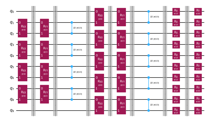 ### เมื่อมี ansatz ที่ลดขนาดแล้วและ observable ที่ขยายออกแล้ว เราสามารถ transpile การทดลองไปยัง Backend ได้ \{#now-that-we-have-our-reduced-ansatze-and-expanded-observables-we-can-transpile-our-experiments-to-the-backend} ที่นี่เราจะใช้ [FakeMelbourneV2](https://quantum.cloud.ibm.com/docs/api/qiskit-ibm-runtime/fake-provider-fake-melbourne-v2) ขนาด 14 Qubit จาก [qiskit-ibm-runtime](https://quantum.cloud.ibm.com/docs/api/qiskit-ibm-runtime) เพื่อสาธิตวิธี transpile ไปยัง QPU Backend ```python from qiskit.transpiler.preset_passmanagers import generate_preset_pass_manager from qiskit_ibm_runtime.fake_provider import FakeMelbourneV2 # Specify a backend and a pass manager for transpilation backend = FakeMelbourneV2() pm = generate_preset_pass_manager(backend=backend, optimization_level=1) # Transpile original experiment circuit_isa = pm.run(circuit) observable_isa = observable.apply_layout(circuit_isa.layout) # Transpile backpropagated experiment bp_circuit_isa = pm.run(bp_circuit) bp_obs_isa = bp_obs.apply_layout(bp_circuit_isa.layout) # Transpile the backpropagated experiment with truncated observable terms bp_circuit_trunc_isa = pm.run(bp_circuit_trunc) bp_obs_trunc_isa = bp_obs_trunc.apply_layout(bp_circuit_trunc_isa.layout) ``` ## ขั้นตอนที่ 3: รัน quantum experiments \{#step-3-execute-quantum-experiments} ### คำนวณค่าความคาดหวัง (expectation value) \{#calculate-expectation-value} สุดท้าย เราสามารถรัน experiment ที่ backpropagate แล้วและเปรียบเทียบกับ experiment แบบเต็มโดยใช้ [StatevectorEstimator](https://quantum.cloud.ibm.com/docs/api/qiskit/qiskit.primitives.StatevectorEstimator) ที่ไม่มี noise จะเห็นว่าค่าความคาดหวัง (expectation value) ที่ได้จาก backpropagation โดยไม่มีการตัดนั้นเทียบเท่ากับค่าที่แม่นตรง (exact value) ภายในขีดจำกัดของความแม่นยำเชิงตัวเลข ค่าความคาดหวัง (expectation value) บน operator ที่มีการตัดพจน์ออกมีความผิดพลาดในระดับ ``1e-4`` ซึ่งอยู่ภายใน tolerance ที่คาดไว้ **หมายเหตุ:** เราใช้ ``Estimator`` primitive แบบ statevector เพื่อแสดงให้เห็นผลของการตัดต่อ output หากต้องการรันบน Backend ที่ transpile ไว้ในขั้นตอนที่ 2 ให้ import [EstimatorV2](https://quantum.cloud.ibm.com/docs/api/qiskit-ibm-runtime/estimator-v2) จาก ``qiskit-ibm-runtime`` แล้วส่ง instance ของ Backend เข้าไปใน constructor ```python from qiskit.primitives import StatevectorEstimator as Estimator estimator = Estimator() # Run the experiments using Estimator primitive result_exact = estimator.run([(circuit_isa, observable_isa)]).result()[0].data.evs.item() result_bp = estimator.run([(bp_circuit_isa, bp_obs_isa)]).result()[0].data.evs.item() result_bp_trunc = ( estimator.run([(bp_circuit_trunc_isa, bp_obs_trunc_isa)]).result()[0].data.evs.item() ) print(f"Exact expectation value: {result_exact}") print(f"Backpropagated expectation value: {result_bp}") print(f"Backpropagated expectation value with truncation: {result_bp_trunc}") print(f" - Expected Error for truncated observable: {metadata.accumulated_error(0):.3e}") print(f" - Observed Error for truncated observable: {abs(result_exact - result_bp_trunc):.3e}") ``` ```text Exact expectation value: 0.8854160687717507 Backpropagated expectation value: 0.8854160687717532 Backpropagated expectation value with truncation: 0.8850236647156059 - Expected Error for truncated observable: 4.933e-02 - Observed Error for truncated observable: 3.924e-04 ``` <TutorialFeedback /> {/* doqumentation-source-hash: 6a2b8207 */}