Qubit Gate และ Circuit ควอนตัม

หมายเหตุ

Kifumi Numata (19 Apr 2024)

คลิก ที่นี่ เพื่อดาวน์โหลด PDF ของบทเรียนต้นฉบับ โปรดทราบว่าโค้ดบางส่วนอาจล้าสมัยไปแล้ว เนื่องจากเป็นภาพนิ่ง

เวลา QPU โดยประมาณสำหรับการรันการทดลองนี้คือ 5 วินาที

1. บทนำ

บิต Gate และ Circuit คือส่วนประกอบพื้นฐานของการคำนวณแบบควอนตัม คุณจะได้เรียนรู้การคำนวณแบบควอนตัมด้วยโมเดลวงจรโดยใช้บิตควอนตัมและ Gate รวมทั้งทบทวนเรื่องซูเปอร์โพสิชัน การวัดค่า และการพันกัน (entanglement)

ในบทเรียนนี้ คุณจะได้เรียนรู้:

• Single-qubit Gate
• Bloch sphere
• ซูเปอร์โพสิชัน
• การวัดค่า
• Two-qubit Gate และสถานะการพันกัน

ในตอนท้ายของบทเรียนนี้ คุณจะได้เรียนรู้เกี่ยวกับความลึกของ Circuit ซึ่งมีความสำคัญอย่างยิ่งสำหรับการคำนวณแบบควอนตัมในระดับ utility scale

2. การคำนวณในรูปแบบไดอะแกรม

เมื่อต้องการใช้งาน Qubit หรือบิต เราต้องจัดการกับมันเพื่อแปลง input ที่มีอยู่ให้เป็น output ที่ต้องการ สำหรับโปรแกรมง่ายๆ ที่มีบิตจำนวนน้อย การแสดงกระบวนการนี้ในรูปแบบไดอะแกรมที่เรียกว่า Circuit diagram จะเป็นประโยชน์มาก

รูปด้านล่างซ้ายเป็นตัวอย่างของ Circuit แบบคลาสสิก ส่วนรูปด้านล่างขวาเป็นตัวอย่างของ Circuit แบบควอนตัม ในทั้งสองกรณี input อยู่ทางซ้ายและ output อยู่ทางขวา ในขณะที่ operation ต่างๆ แสดงด้วยสัญลักษณ์ สัญลักษณ์ที่ใช้สำหรับ operation เหล่านี้เรียกว่า "Gate" ซึ่งส่วนใหญ่เป็นชื่อที่มาจากประวัติศาสตร์

3. Single-qubit quantum Gate

3.1 สถานะควอนตัมและ Bloch sphere

สถานะของ Qubit แสดงในรูปแบบซูเปอร์โพสิชันของ $|0\rangle$ และ $|1\rangle$ สถานะควอนตัมทั่วไปแสดงได้ดังนี้

$$|\psi\rangle =\alpha|0\rangle+ \beta|1\rangle$$

โดยที่ $\alpha$ และ $\beta$ เป็นจำนวนเชิงซ้อนที่มีคุณสมบัติ $|\alpha|^2+|\beta|^2=1$

$|0\rangle$ และ $|1\rangle$ เป็นเวกเตอร์ในปริภูมิเวกเตอร์เชิงซ้อนสองมิติ:

$$|0\rangle = \begin{pmatrix} 1 \\0 \end{pmatrix}, |1\rangle = \begin{pmatrix} 0\\1 \end{pmatrix}$$

ดังนั้น สถานะควอนตัมทั่วไปสามารถแสดงได้ในรูป

$$|\psi\rangle = \alpha\begin{pmatrix} 1 \\ 0 \end{pmatrix} + \beta\begin{pmatrix}0\\ 1 \end{pmatrix} = \begin{pmatrix} \alpha \\ \beta \end{pmatrix}$$

จากนี้จะเห็นว่าสถานะของบิตควอนตัมคือเวกเตอร์หน่วยในปริภูมิผลคูณภายในเชิงซ้อนสองมิติ ที่มีฐานออร์โธนอร์มอลเป็น $|0\rangle$ และ $|1\rangle$ โดย normalize ให้เท่ากับ 1

$$\langle\psi|\psi\rangle = \begin{pmatrix} \alpha^* & \beta^* \end{pmatrix} \begin{pmatrix} \alpha \\ \beta \end{pmatrix} = 1$$

|\psi\rangle =\begin\{pmatrix\} \alpha \\ \beta \end\{pmatrix\} ยังถูกเรียกว่า statevector ด้วย

สถานะควอนตัม single-qubit ยังสามารถแสดงได้ในรูป

$$|\psi\rangle =\cos\frac{\theta}{2}|0\rangle+e^{i\varphi}\sin\frac{\theta}{2}|1\rangle =\left( \begin{pmatrix} \cos\frac{\theta}{2}\\ e^{i\varphi}\sin\frac{\theta}{2} \end{pmatrix}\right)$$

โดยที่ $\theta$ และ $\varphi$ คือมุมของ Bloch sphere ในรูปด้านล่าง

ในเซลล์โค้ดถัดไป เราจะสร้างการคำนวณพื้นฐานจากชิ้นส่วนต่างๆ ใน Qiskit ทีละขั้น เราจะสร้าง Circuit ว่างแล้วเพิ่ม operation ควอนตัมเข้าไป พร้อมอธิบาย Gate ต่างๆ และแสดงผลด้วยภาพระหว่างทาง สามารถรันเซลล์ได้โดยกด "Shift" + "Enter" นำเข้า library ก่อนเลย

# Added by doQumentation — required packages for this notebook
!pip install -q qiskit qiskit-aer qiskit-ibm-runtime

# Import the qiskit library
from qiskit import QuantumCircuit
from qiskit_aer import AerSimulator
from qiskit.quantum_info import Statevector
from qiskit.visualization import plot_bloch_multivector
from qiskit_ibm_runtime import Sampler
from qiskit.transpiler.preset_passmanagers import generate_preset_pass_manager
from qiskit.visualization import plot_histogram

เตรียม Circuit ควอนตัม

เราจะสร้างและแสดง Circuit แบบ single-qubit

# Create the single-qubit quantum circuit
qc = QuantumCircuit(1)

# Draw the circuit
qc.draw("mpl")

X Gate

X Gate คือการหมุน $\pi$ รอบแกน $x$ ของ Bloch sphere การใช้ X Gate กับ $|0\rangle$ จะได้ $|1\rangle$ และการใช้ X Gate กับ $|1\rangle$ จะได้ $|0\rangle$ ดังนั้น มันจึงเป็น operation ที่คล้ายกับ NOT Gate ในแบบคลาสสิก และยังเป็นที่รู้จักในชื่อ bit flip ด้วย การแสดงเมทริกซ์ของ X Gate แสดงด้านล่าง

$$X = \begin{pmatrix} 0 & 1 \\ 1 & 0 \\ \end{pmatrix}$$

qc = QuantumCircuit(1)  # Prepare the single-qubit quantum circuit

# Apply a X gate to qubit 0
qc.x(0)

# Draw the circuit
qc.draw("mpl")

ใน IBM Quantum® สถานะเริ่มต้นถูกกำหนดให้เป็น $|0\rangle$ ดังนั้น Circuit ควอนตัมด้านบนในรูปแบบเมทริกซ์คือ

$$X|0\rangle= \begin{pmatrix} 0 & 1 \\ 1 & 0 \end{pmatrix} \begin{pmatrix} 1 \\ 0 \end{pmatrix} =\begin{pmatrix} 0 \\ 1 \end{pmatrix} = |1\rangle$$

ต่อไป ลองรัน Circuit นี้โดยใช้ statevector simulator กัน

# See the statevector
out_vector = Statevector(qc)
print(out_vector)

# Draw a Bloch sphere
plot_bloch_multivector(out_vector)

Statevector([0.+0.j, 1.+0.j],
            dims=(2,))

เวกเตอร์แนวตั้งแสดงเป็นเวกเตอร์แถว โดยมีจำนวนเชิงซ้อน (ส่วนจินตภาพใช้ดัชนี $j$)

H Gate

Hadamard Gate คือการหมุน $\pi$ รอบแกนที่อยู่กึ่งกลางระหว่างแกน $x$ และ $z$ บน Bloch sphere การใช้ H Gate กับ $|0\rangle$ จะสร้างสถานะซูเปอร์โพสิชัน เช่น $\frac{|0\rangle + |1\rangle}{\sqrt{2}}$ การแสดงเมทริกซ์ของ H Gate แสดงด้านล่าง

$$H = \frac{1}{\sqrt{2}}\begin{pmatrix} 1 & 1 \\ 1 & -1 \\ \end{pmatrix}$$

qc = QuantumCircuit(1)  # Create the single-qubit quantum circuit

# Apply an Hadamard gate to qubit 0
qc.h(0)

# Draw the circuit
qc.draw(output="mpl")

# See the statevector
out_vector = Statevector(qc)
print(out_vector)

# Draw a Bloch sphere
plot_bloch_multivector(out_vector)

Statevector([0.70710678+0.j, 0.70710678+0.j],
            dims=(2,))

นั่นคือ

$$H|0\rangle= \frac{1}{\sqrt{2}} \begin{pmatrix} 1 & 1 \\ 1 & -1 \end{pmatrix} \begin{pmatrix} 1 \\0 \end{pmatrix} =\frac{1}{\sqrt{2}}\begin{pmatrix} 1 \\ 1 \end{pmatrix} =\begin{pmatrix} 0.707 \\ 0.707 \end{pmatrix} =\frac{1}{\sqrt{2}}(|0\rangle+|1\rangle)$$

สถานะซูเปอร์โพสิชันนี้พบบ่อยและสำคัญมาก จนได้รับสัญลักษณ์เป็นของตัวเอง:

$$|+\rangle \equiv \frac{1}{\sqrt{2}}(|0\rangle+|1\rangle).$$

การใช้ $H$ Gate กับ $|0\rangle$ ทำให้เกิดซูเปอร์โพสิชันของ $|0\rangle$ และ $|1\rangle$ โดยการวัดค่าในฐานการคำนวณ (ตามแกน z ใน Bloch sphere) จะให้แต่ละสถานะด้วยความน่าจะเป็นที่เท่ากัน

สถานะ $|-\rangle$

คุณอาจเดาได้แล้วว่ามีสถานะ $|-\rangle$ ที่สอดคล้องกัน:

$$|-\rangle \equiv \frac{|0\rangle -|1\rangle}{\sqrt{2}}.$$

เพื่อสร้างสถานะนี้ ให้ใช้ X Gate ก่อนเพื่อให้ได้ $|1\rangle$ แล้วตามด้วย H Gate

qc = QuantumCircuit(1)  # Create the single-qubit quantum circuit

# Apply a X gate to qubit 0
qc.x(0)

# Apply an Hadamard gate to qubit 0
qc.h(0)

# draw the circuit
qc.draw(output="mpl")

# See the statevector
out_vector = Statevector(qc)
print(out_vector)

# Draw a Bloch sphere
plot_bloch_multivector(out_vector)

Statevector([ 0.70710678+0.j, -0.70710678+0.j],
            dims=(2,))

นั่นคือ

$$H|1\rangle= \frac{1}{\sqrt{2}} \begin{pmatrix} 1 & 1 \\\ 1 & -1 \end{pmatrix} \begin{pmatrix} 0 \\\ 1 \end{pmatrix} =\frac{1}{\sqrt{2}}\begin{pmatrix} 1 \\\ -1 \end{pmatrix} =\begin{pmatrix} 0.707 \\\ -0.707 \end{pmatrix} =\frac{1}{\sqrt{2}}(|0\rangle-|1\rangle) = |-\rangle$$

การใช้ $H$ Gate กับ $|1\rangle$ ทำให้ได้ซูเปอร์โพสิชันที่เท่ากันของ $|0\rangle$ และ $|1\rangle$ แต่เครื่องหมายของ $|1\rangle$ เป็นลบ

3.2 สถานะควอนตัม single-qubit และการวิวัฒนาการแบบยูนิทารี

การกระทำของ Gate ทุกตัวที่เราเห็นมาจนถึงตอนนี้ล้วนเป็น unitary ซึ่งหมายความว่าสามารถแสดงด้วยตัวดำเนินการยูนิทารีได้ กล่าวอีกนัยหนึ่ง สถานะ output สามารถได้มาโดยการกระทำสถานะเริ่มต้นด้วยเมทริกซ์ยูนิทารี:

$$|\psi^{'}\rangle = U|\psi\rangle$$

เมทริกซ์ยูนิทารีคือเมทริกซ์ที่ตอบสนอง

$$U^{\dagger}U =U U^{\dagger} = I.$$

ในแง่ของการทำงานของคอมพิวเตอร์ควอนตัม เราจะกล่าวว่าการใช้ quantum Gate กับ Qubit จะทำให้สถานะควอนตัมวิวัฒนาการไป Single-qubit Gate ที่พบบ่อยได้แก่ดังต่อไปนี้

Pauli Gate:

$$X = \begin{pmatrix} 0 & 1 \\ 1 & 0 \\ \end{pmatrix} = |0\rangle \langle 1|+|1\rangle \langle 0|$$ $$Y = \begin{pmatrix} 0 & -i \\ i & 0 \\ \end{pmatrix} = -i|0\rangle \langle 1|+i|1\rangle \langle 0|$$ $$Z = \begin{pmatrix} 1 & 0 \\ 0 & -1 \\ \end{pmatrix} = |0\rangle \langle 0|-|1\rangle \langle 1|$$

โดยที่ผลคูณแบบ outer product คำนวณได้ดังนี้:

$$|0\rangle \langle 0|= \begin{bmatrix} 1 \\ 0 \end{bmatrix} \begin{bmatrix} 1 & 0 \end{bmatrix} =\begin{bmatrix} 1 & 0 \\ 0 & 0 \\ \end{bmatrix}, \quad |1\rangle \langle 0|= \begin{bmatrix} 0 \\ 1 \end{bmatrix} \begin{bmatrix} 1 & 0 \end{bmatrix} =\begin{bmatrix} 0 & 0 \\ 1 & 0 \\ \end{bmatrix}, \quad$$ $$|0\rangle \langle 1|= \begin{bmatrix} 1 \\ 0 \end{bmatrix} \begin{bmatrix} 0 & 1 \end{bmatrix} =\begin{bmatrix} 0 & 1 \\ 0 & 0 \\ \end{bmatrix}, \quad |1\rangle \langle 1|= \begin{bmatrix} 0 \\ 1 \end{bmatrix} \begin{bmatrix} 0 & 1 \end{bmatrix} =\begin{bmatrix} 0 & 0 \\ 0 & 1 \\ \end{bmatrix}, \quad$$

Single-qubit Gate ทั่วไปอื่นๆ:

$$H= \frac{1}{\sqrt{2}}\begin{bmatrix} 1 & 1 \\ 1 & -1 \\ \end{bmatrix},\quad S = \begin{bmatrix} 1 & 0 \\ 0 & i \\ \end{bmatrix}, \quad T = \begin{bmatrix} 1 & 0 \\ 0 & exp(i\pi/4) \\ \end{bmatrix}$$ $$R_x(\theta) = e^{-i\theta X/2} = cos\frac{\theta}{2}I - i sin \frac{\theta}{2}X = \begin{bmatrix} cos\frac{\theta}{2} & -i sin \frac{\theta}{2} \\ -i sin \frac{\theta}{2} & cos\frac{\theta}{2} \\ \end{bmatrix}$$ $$R_y(\theta) = e^{-i\theta Y/2} = cos\frac{\theta}{2}I - i sin \frac{\theta}{2}Y = \begin{bmatrix} cos\frac{\theta}{2} & - sin \frac{\theta}{2} \\ sin \frac{\theta}{2} & cos\frac{\theta}{2} \\ \end{bmatrix}$$ $$R_z(\theta) = e^{-i\theta Z/2} = cos\frac{\theta}{2}I - i sin \frac{\theta}{2}Z = \begin{bmatrix} e^{-i\theta /2} & 0 \\ 0 & e^{i\theta /2} \\ \end{bmatrix}$$

ความหมายและการใช้งานของ Gate เหล่านี้อธิบายอย่างละเอียดในหลักสูตร Basics of Quantum Information

แบบฝึกหัดที่ 1

ใช้ Qiskit เพื่อสร้าง Circuit ควอนตัมที่เตรียมสถานะที่อธิบายด้านล่าง จากนั้นรัน Circuit แต่ละอันโดยใช้ statevector simulator และแสดงสถานะผลลัพธ์บน Bloch sphere โบนัส: ลองคาดเดาว่าสถานะสุดท้ายควรเป็นอะไรจากความเข้าใจเรื่อง Gate และการหมุนบน Bloch sphere

(1) $XX|0\rangle$

(2) $HH|0\rangle$

(3) $HZH|0\rangle$

เคล็ดลับ: Z Gate ใช้งานได้ด้วย

qc.z(0)

วิธีแก้:

### (1) XX|0> ###

# Create the single-qubit quantum circuit
qc = QuantumCircuit(1)  ##your code goes here##

# Add a X gate to qubit 0
qc.x(0)  ##your code goes here##

# Add a X gate to qubit 0
qc.x(0)  ##your code goes here##

# Draw a circuit
qc.draw(output="mpl")

# See the statevector
out_vector = Statevector(qc)
print(out_vector)

# Draw a Bloch sphere
plot_bloch_multivector(out_vector)

Statevector([1.+0.j, 0.+0.j],
            dims=(2,))

### (2) HH|0> ###
##your code goes here##
qc = QuantumCircuit(1)
qc.h(0)
qc.h(0)
qc.draw("mpl")

# See the statevector
out_vector = Statevector(qc)
print(out_vector)

# Draw a Bloch sphere
plot_bloch_multivector(out_vector)

Statevector([1.+0.j, 0.+0.j],
            dims=(2,))

### (3) HZH|0> ###
##your code goes here##
qc = QuantumCircuit(1)
qc.h(0)
qc.z(0)
qc.h(0)
qc.draw("mpl")

# See the statevector
out_vector = Statevector(qc)
print(out_vector)

# Draw a Bloch sphere
plot_bloch_multivector(out_vector)

Statevector([0.+0.j, 1.+0.j],
            dims=(2,))

3.3 การวัดค่า

การวัดค่าเป็นหัวข้อที่ซับซ้อนมากในเชิงทฤษฎี แต่ในทางปฏิบัติ การวัดตามแกน $z$ (ซึ่งคอมพิวเตอร์ควอนตัม IBM® ทุกเครื่องทำ) จะบังคับให้สถานะ $\alpha|0\rangle+\beta|1\rangle \quad (s.t.|\alpha|^2+|\beta|^2=1)$ ของ Qubit เป็นได้แค่ $|0\rangle$ หรือ $|1\rangle$ และเราสังเกตผลลัพธ์

• $|\alpha|^2$ คือความน่าจะเป็นที่เราจะได้ $|0\rangle$ เมื่อวัดค่า
• $|\beta|^2$ คือความน่าจะเป็นที่เราจะได้ $|1\rangle$ เมื่อวัดค่า

ดังนั้น $\alpha$ และ $\beta$ จึงเรียกว่า probability amplitude (ดู "Born rule")

ตัวอย่างเช่น $\frac{\sqrt{2}}{2}|0\rangle+\frac{\sqrt{2}}{2}|1\rangle$ มีความน่าจะเป็นเท่ากันที่จะกลายเป็น $|0\rangle$ หรือ $|1\rangle$ เมื่อวัดค่า ส่วน $\frac{\sqrt{3}}{2}|0\rangle-\frac{1}{2}i|1\rangle$ มีโอกาส 75% ที่จะกลายเป็น $|0\rangle$

Qiskit Aer Simulator

ต่อไป ลองวัดค่า Circuit ที่เตรียมซูเปอร์โพสิชันความน่าจะเป็นเท่ากันด้านบน เราต้องเพิ่ม measurement Gate เข้าไป เนื่องจาก Qiskit Aer simulator จำลองฮาร์ดแวร์ควอนตัมในอุดมคติ (ไม่มี noise) โดยค่าเริ่มต้น หมายเหตุ: Aer simulator ยังสามารถใช้ noise model ที่อ้างอิงจากคอมพิวเตอร์ควอนตัมจริงได้ เราจะกลับมาพูดถึง noise model ในภายหลัง

# Create a new circuit with one qubits (first argument) and one classical bits (second argument)
qc = QuantumCircuit(1, 1)
qc.h(0)
qc.measure(0, 0)  # Add the measurement gate

qc.draw(output="mpl")

ตอนนี้เราพร้อมรัน Circuit บน Aer simulator แล้ว ในตัวอย่างนี้เราจะใช้ค่าเริ่มต้น shots=1024 ซึ่งหมายความว่าเราจะวัดค่า 1024 ครั้ง จากนั้นเราจะ plot ผลนั้นในรูปแบบ histogram

# Run the circuit on a simulator to get the results
# Define backend
backend = AerSimulator()

# Transpile to backend
pm = generate_preset_pass_manager(backend=backend, optimization_level=1)
isa_qc = pm.run(qc)

# Run the job
sampler = Sampler(mode=backend)
job = sampler.run([isa_qc])
result = job.result()

# Print the results
counts = result[0].data.c.get_counts()
print(counts)

# Plot the counts in a histogram
plot_histogram(counts)

{'0': 521, '1': 503}

เราจะเห็นว่า 0 และ 1 ถูกวัดได้ด้วยความน่าจะเป็นเกือบ 50% แต่ละค่า แม้ว่าจะไม่ได้จำลอง noise ในที่นี้ แต่สถานะก็ยังมีความน่าจะเป็น ดังนั้นแม้จะคาดว่าจะได้การกระจายแบบ 50-50 แต่เราแทบไม่พบสัดส่วนที่เท่ากันพอดีทุกครั้ง เหมือนกับการโยนเหรียญ 100 ครั้งที่ไม่ค่อยได้หัว-ก้อย 50 ครั้งพอดีแต่ละด้าน

4. Multi-qubit quantum Gate และการพันกัน

4.1 Multi-qubit quantum Circuit

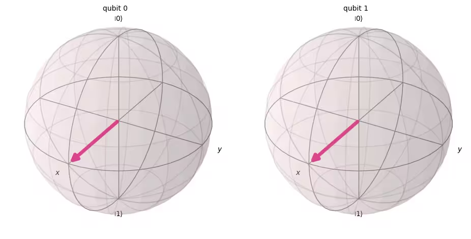
เราสามารถสร้าง Circuit ควอนตัมแบบ two-qubit ได้ด้วยโค้ดต่อไปนี้ เราจะใช้ H Gate กับแต่ละ Qubit

# Create the two qubits quantum circuit
qc = QuantumCircuit(2)

# Apply an H gate to qubit 0
qc.h(0)

# Apply an H gate to qubit 1
qc.h(1)

# Draw the circuit
qc.draw(output="mpl")

# See the statevector
out_vector = Statevector(qc)
print(out_vector)

Statevector([0.5+0.j, 0.5+0.j, 0.5+0.j, 0.5+0.j],
            dims=(2, 2))

หมายเหตุ: การเรียงลำดับบิตใน Qiskit

Qiskit ใช้สัญกรณ์ Little Endian ในการเรียงลำดับ Qubit และบิต ซึ่งหมายความว่า Qubit 0 คือบิตขวาสุด ในสตริงบิต ตัวอย่าง: $|01\rangle$ หมายความว่า q0 เป็น $|1\rangle$ และ q1 เป็น $|0\rangle$ ต้องระวังเพราะวรรณกรรมบางส่วนในการคำนวณแบบควอนตัมใช้สัญกรณ์ Big Endian (Qubit 0 คือบิตซ้ายสุด) รวมถึงวรรณกรรมกลศาสตร์ควอนตัมจำนวนมากก็ใช้เช่นกัน

สิ่งที่ควรสังเกตอีกอย่างคือเมื่อแสดง Circuit ควอนตัม $|q_0\rangle$ จะอยู่ด้านบนของ Circuit เสมอ เมื่อคำนึงถึงเรื่องนี้ สถานะควอนตัมของ Circuit ด้านบนสามารถเขียนเป็น tensor product ของสถานะควอนตัม single-qubit ได้

$|q1\rangle \otimes|q0\rangle = (a|0\rangle+b|1\rangle) \otimes (c|0\rangle+d|1\rangle)$

$= ac|0\rangle|0\rangle+ad|0\rangle|1\rangle+bc|1\rangle|0\rangle+bd|1\rangle|1\rangle$

$= ac|00\rangle+ad|01\rangle+bc|10\rangle+bd|11\rangle$

( $|ac|^2+ |ad|^2+ |bc|^2+ |bd|^2=1$ )

สถานะเริ่มต้นของ Qiskit คือ $|0\rangle|0\rangle=|00\rangle$ ดังนั้นเมื่อใช้ $H$ กับ Qubit แต่ละตัว จะเปลี่ยนเป็นสถานะซูเปอร์โพสิชันที่เท่ากัน

$H|0\rangle \otimes H|0\rangle=\frac{1}{\sqrt{2}}(|0\rangle+|1\rangle) \otimes \frac{1}{\sqrt{2}}(|0\rangle+|1\rangle) = \frac{1}{2}(|00\rangle+|01\rangle+|10\rangle+|11\rangle)$

$$=\frac{1}{2}\left( \begin{pmatrix} 1 \\ 1 \end{pmatrix} \otimes \begin{pmatrix} 1 \\ 1 \end{pmatrix}\right) = \frac{1}{2}\begin{pmatrix} 1 \\ 1 \\ 1 \\ 1 \end{pmatrix}=\frac{1}{2}\left(\begin{pmatrix} 1 \\ 0 \\ 0 \\ 0 \end{pmatrix}+\begin{pmatrix} 0 \\ 1 \\ 0 \\ 0 \end{pmatrix}+\begin{pmatrix} 0 \\ 0 \\ 1 \\ 0 \end{pmatrix}+\begin{pmatrix} 0 \\ 0 \\ 0 \\ 1 \end{pmatrix}\right)$$

กฎการวัดค่าก็เหมือนกับกรณี single-qubit คือความน่าจะเป็นในการวัด $|00\rangle$ คือ $|ac|^2$

# Draw a Bloch sphere
plot_bloch_multivector(out_vector)

ต่อไป ลองวัดค่า Circuit นี้กัน

# Create a new circuit with two qubits (first argument) and two classical bits (second argument)
qc = QuantumCircuit(2, 2)

# Apply the gates
qc.h(0)
qc.h(1)

# Add the measurement gates
qc.measure(0, 0)  # Measure qubit 0 and save the result in bit 0
qc.measure(1, 1)  # Measure qubit 1 and save the result in bit 1

# Draw the circuit
qc.draw(output="mpl")

ตอนนี้เราจะใช้ Aer simulator อีกครั้งเพื่อยืนยันในเชิงทดลองว่าความน่าจะเป็นสัมพัทธ์ของสถานะ output ที่เป็นไปได้ทั้งหมดมีค่าใกล้เคียงกัน

# Run the circuit on a simulator to get the results
# Define backend
backend = AerSimulator()

# Transpile to backend
pm = generate_preset_pass_manager(backend=backend, optimization_level=1)
isa_qc = pm.run(qc)

# Run the job
sampler = Sampler(mode=backend)
job = sampler.run([isa_qc])
result = job.result()

# Print the results
counts = result[0].data.c.get_counts()
print(counts)

# Plot the counts in a histogram
plot_histogram(counts)

{'10': 262, '01': 246, '00': 265, '11': 251}

ตามที่คาดไว้ สถานะ $|00\rangle$, $|01\rangle$, $|10\rangle$, $|11\rangle$ ถูกวัดได้ประมาณ 25% แต่ละสถานะ

4.2 Multi-qubit quantum Gate

CNOT Gate

CNOT Gate ("controlled NOT" หรือ CX) คือ Gate แบบ two-qubit ซึ่งหมายความว่าการกระทำของมันเกี่ยวข้องกับ Qubit สองตัวพร้อมกัน: control qubit และ target qubit CNOT จะพลิก target qubit เมื่อ control qubit เป็น $|1\rangle$ เท่านั้น

Input (target,control)	Output (target,control)
00	00
01	11
10	10
11	01

ลองจำลองการกระทำของ Gate แบบ two-qubit นี้ก่อน เมื่อ q0 และ q1 เป็น $|0\rangle$ ทั้งคู่ แล้วดูผล statevector ที่ได้ ไวยากรณ์ Qiskit ที่ใช้คือ qc.cx(control qubit, target qubit)

# Create a circuit with two quantum registers and two classical registers
qc = QuantumCircuit(2, 2)

# Apply the CNOT (cx) gate to a |00> state.
qc.cx(0, 1)  # Here the control is set to q0 and the target is set to q1.

# Draw the circuit
qc.draw(output="mpl")

# See the statevector
out_vector = Statevector(qc)
print(out_vector)

Statevector([1.+0.j, 0.+0.j, 0.+0.j, 0.+0.j],
            dims=(2, 2))

ตามที่คาดไว้ การใช้ CNOT Gate กับ $|00\rangle$ ไม่เปลี่ยนสถานะ เนื่องจาก control qubit อยู่ในสถานะ $|0\rangle$ กลับมาที่ CNOT operation ของเรา คราวนี้เราจะใช้ CNOT Gate กับ $|01\rangle$ แล้วดูว่าเกิดอะไรขึ้น

qc = QuantumCircuit(2, 2)

# q0=1, q1=0
qc.x(0)  # Apply a X gate to initialize q0 to 1
qc.cx(0, 1)  # Set the control bit to q0 and the target bit to q1.

# Draw the circuit
qc.draw(output="mpl")

# See the statevector
out_vector = Statevector(qc)
print(out_vector)

Statevector([0.+0.j, 0.+0.j, 0.+0.j, 1.+0.j],
            dims=(2, 2))

การใช้ CNOT Gate ทำให้สถานะ $|01\rangle$ กลายเป็น $|11\rangle$

ลองยืนยันผลเหล่านี้โดยรัน Circuit บน simulator

# Add measurements
qc.measure(0, 0)
qc.measure(1, 1)

# Draw the circuit
qc.draw(output="mpl")

# Run the circuit on a simulator to get the results
# Define backend
backend = AerSimulator()

# Transpile to backend
pm = generate_preset_pass_manager(backend=backend, optimization_level=1)
isa_qc = pm.run(qc)

# Run the job
sampler = Sampler(backend)
job = sampler.run([isa_qc])
result = job.result()

# Print the results
counts = result[0].data.c.get_counts()
print(counts)

# Plot the counts in a histogram
plot_histogram(counts)

{'11': 1024}

ผลลัพธ์ควรแสดงว่า $|11\rangle$ ถูกวัดได้ด้วยความน่าจะเป็น 100%

4.3 การพันกันของควอนตัมและการรันบนอุปกรณ์ควอนตัมจริง

เริ่มต้นด้วยการแนะนำสถานะพันกันที่เฉพาะเจาะจงซึ่งมีความสำคัญอย่างยิ่งในการคำนวณแบบควอนตัม แล้วเราจะนิยามคำว่า "entangled":

$$\frac{1}{\sqrt{2}}|00\rangle + \frac{1}{\sqrt{2}}|11\rangle$$

และสถานะนี้เรียกว่า Bell state

สถานะพันกันคือสถานะ $|\psi_{AB}\rangle$ ที่ประกอบด้วยสถานะควอนตัม $|\psi_A\rangle$ และ $|\psi_B\rangle$ ซึ่งไม่สามารถแสดงเป็น tensor product ของสถานะควอนตัมแต่ละตัวได้

ถ้า $|\psi_{AB}\rangle$ ด้านล่างมีสถานะสองสถานะ $|\psi\rangle_A$ และ $|\psi\rangle_B$;

$$|\psi_{AB}\rangle = \frac{1}{\sqrt{2}}(|00\rangle +|11\rangle) = \frac{1}{\sqrt{2}}(|0\rangle_A|0\rangle_B +|1\rangle_A|1\rangle_B)$$ $$|\psi\rangle_A = a_0|0\rangle+a_1|1\rangle$$ $$|\psi\rangle_B = b_0|0\rangle+b_1|1\rangle$$

tensor product ของสองสถานะนี้คือ

$$|\psi\rangle _A\otimes |\psi\rangle _B = a_0 b_0|00\rangle+a_0 b_1|01\rangle+a_1 b_0|10\rangle+a_1 b_1|11\rangle$$

แต่ไม่มีสัมประสิทธิ์ $a_0, a_1, b_0,$ และ $b_1$ ที่จะทำให้สมการทั้งสองนี้เป็นจริงได้ ดังนั้น $|\psi_{AB}\rangle$ จึงไม่สามารถแสดงเป็น tensor product ของสถานะควอนตัมแต่ละตัว $|\psi\rangle_A$ และ $|\psi\rangle_B$ ได้ และนั่นหมายความว่า $|\psi_{AB}\rangle = \frac{1}{\sqrt{2}}(|00\rangle +|11\rangle)$ คือสถานะพันกัน

ลองสร้าง Bell state และรันบนคอมพิวเตอร์ควอนตัมจริง ตอนนี้เราจะทำตามสี่ขั้นตอนในการเขียนโปรแกรมควอนตัม ที่เรียกว่า Qiskit patterns:

1. Map ปัญหาไปยัง Circuit และตัวดำเนินการควอนตัม
2. Optimize สำหรับฮาร์ดแวร์เป้าหมาย
3. Execute บนฮาร์ดแวร์เป้าหมาย
4. Post-process ผลลัพธ์

ขั้นตอนที่ 1. Map ปัญหาไปยัง Circuit และตัวดำเนินการควอนตัม

ในโปรแกรมควอนตัม Circuit ควอนตัมคือรูปแบบดั้งเดิมในการแสดงคำสั่งควอนตัม เมื่อสร้าง Circuit คุณมักจะสร้าง object QuantumCircuit ใหม่ แล้วเพิ่มคำสั่งเข้าไปตามลำดับ

เซลล์โค้ดต่อไปนี้สร้าง Circuit ที่ผลิต Bell state ซึ่งเป็นสถานะพันกัน two-qubit ที่เฉพาะเจาะจงด้านบน

qc = QuantumCircuit(2, 2)

qc.h(0)
qc.cx(0, 1)

qc.measure(0, 0)
qc.measure(1, 1)

qc.draw("mpl")

ขั้นตอนที่ 2. Optimize สำหรับฮาร์ดแวร์เป้าหมาย

Qiskit แปลง Circuit นามธรรมเป็น Circuit แบบ QISA (Quantum Instruction Set Architecture) ที่เคารพข้อจำกัดของฮาร์ดแวร์เป้าหมายและ optimize ประสิทธิภาพของ Circuit ดังนั้นก่อนการ optimize เราจะระบุฮาร์ดแวร์เป้าหมาย ถ้าคุณไม่มี qiskit-ibm-runtime คุณต้องติดตั้งก่อน สำหรับข้อมูลเพิ่มเติมเกี่ยวกับ Qiskit Runtime ดูที่ API reference

# Install
# !pip install qiskit-ibm-runtime

เราจะระบุฮาร์ดแวร์เป้าหมาย

from qiskit_ibm_runtime import QiskitRuntimeService

service = QiskitRuntimeService()
service.backends()

# You can specify the device
# backend = service.backend('ibm_kingston')

# You can also identify the least busy device
backend = service.least_busy(operational=True)
print("The least busy device is ", backend)

การ Transpile Circuit เป็นกระบวนการที่ซับซ้อนอีกขั้นหนึ่ง โดยสรุปสั้นๆ คือการเขียน Circuit ใหม่ให้เทียบเท่าทางตรรกะโดยใช้ "native gate" (Gate ที่คอมพิวเตอร์ควอนตัมเฉพาะตัวสามารถทำได้) และ map Qubit ใน Circuit ของคุณไปยัง Qubit จริงที่เหมาะสมบนคอมพิวเตอร์ควอนตัมเป้าหมาย สำหรับข้อมูลเพิ่มเติมเกี่ยวกับการ transpilation ดูเอกสารนี้

# Transpile the circuit into basis gates executable on the hardware
pm = generate_preset_pass_manager(backend=backend, optimization_level=1)
target_circuit = pm.run(qc)

target_circuit.draw("mpl", idle_wires=False)

คุณจะเห็นว่าในการ transpilation นั้น Circuit ถูกเขียนใหม่โดยใช้ Gate ใหม่ สำหรับข้อมูลเพิ่มเติม ดูเอกสาร ECRGate

ขั้นตอนที่ 3. Execute target circuit

ตอนนี้เราจะรัน target circuit บนอุปกรณ์จริง

sampler = Sampler(backend)
job_real = sampler.run([target_circuit])

job_id = job_real.job_id()
print("job id:", job_id)

การรันบนอุปกรณ์จริงอาจต้องรอในคิว เนื่องจากคอมพิวเตอร์ควอนตัมเป็นทรัพยากรที่มีคุณค่าและเป็นที่ต้องการมาก job_id ใช้สำหรับตรวจสอบสถานะการรันและผลลัพธ์ของ job ในภายหลัง

# Check the job status (replace the job id below with your own)
job_real.status(job_id)

คุณยังสามารถตรวจสอบสถานะ job ได้จาก IBM Quantum dashboard：https://quantum.cloud.ibm.com/workloads

# If the Notebook session got disconnected you can also check your job status
# by running the following code
from qiskit_ibm_runtime import QiskitRuntimeService

service = QiskitRuntimeService()
job_real = service.job(job_id)  # Input your job-id between the quotations
job_real.status()

# Execute after job has successfully run
result_real = job_real.result()
print(result_real[0].data.c.get_counts())

ขั้นตอนที่ 4. Post-process ผลลัพธ์

สุดท้าย เราต้อง post-process ผลลัพธ์เพื่อสร้าง output ในรูปแบบที่ต้องการ เช่น ค่าหรือกราฟ

plot_histogram(result_real[0].data.c.get_counts())

อย่างที่เห็น $|00\rangle$ และ $|11\rangle$ ถูกสังเกตพบบ่อยที่สุด มีผลลัพธ์บางส่วนนอกเหนือจากข้อมูลที่คาดไว้ ซึ่งเกิดจาก noise และการ decoherence ของ Qubit เราจะได้เรียนรู้เพิ่มเติมเกี่ยวกับ error และ noise ในคอมพิวเตอร์ควอนตัมในบทเรียนถัดๆ ไปของหลักสูตรนี้

4.4 GHZ state

แนวคิดของการพันกันสามารถขยายไปยังระบบที่มี Qubit มากกว่าสอง GHZ state (Greenberger-Horne-Zeilinger state) คือสถานะพันกันสูงสุดของ Qubit สามตัวหรือมากกว่า GHZ state สำหรับ Qubit สามตัวนิยามดังนี้

$$\frac{1}{\sqrt 2}(|000\rangle + |111\rangle)$$

สามารถสร้างได้ด้วย Circuit ควอนตัมต่อไปนี้

qc = QuantumCircuit(3, 3)

qc.h(0)
qc.cx(0, 1)
qc.cx(1, 2)

qc.measure(0, 0)
qc.measure(1, 1)
qc.measure(2, 2)

qc.draw("mpl")

"ความลึก" ของ Circuit ควอนตัมเป็นตัวชี้วัดที่มีประโยชน์และพบบ่อยในการอธิบาย Circuit ควอนตัม ลองเดิน path ผ่าน Circuit ควอนตัม โดยเคลื่อนจากซ้ายไปขวา และเปลี่ยน Qubit เฉพาะเมื่อมี multi-qubit Gate เชื่อมต่อกันเท่านั้น นับจำนวน Gate ตาม path นั้น จำนวน Gate สูงสุดสำหรับ path ใดๆ ผ่าน Circuit คือความลึก ในคอมพิวเตอร์ควอนตัมที่มี noise ในยุคปัจจุบัน Circuit ที่มีความลึกน้อยจะมี error น้อยกว่าและมักให้ผลลัพธ์ที่ดี Circuit ที่ลึกมากไม่เป็นเช่นนั้น

การใช้ QuantumCircuit.depth() ทำให้เราตรวจสอบความลึกของ Circuit ควอนตัมได้ ความลึกของ Circuit ด้านบนคือ 4 Qubit บนสุดมีแค่สาม Gate รวมถึงการวัดค่า แต่มี path จาก Qubit บนสุดลงไปยัง Qubit 1 หรือ Qubit 2 ที่ผ่าน CNOT Gate อีกตัว

qc.depth()

4

แบบฝึกหัดที่ 2

GHZ state ของระบบ 8-Qubit คือ

$$\frac{1}{\sqrt 2}(|00000000\rangle + |11111111\rangle)$$

เขียนโค้ดเพื่อเตรียมสถานะนี้ด้วย Circuit ที่ตื้นที่สุดที่เป็นไปได้ ความลึกของ Circuit ควอนตัมที่ตื้นที่สุดคือ 5 รวมถึง measurement Gate

วิธีแก้:

# Step 1
qc = QuantumCircuit(8, 8)

##your code goes here##
qc.h(0)
qc.cx(0, 4)
qc.cx(4, 6)
qc.cx(6, 7)

qc.cx(4, 5)

qc.cx(0, 2)
qc.cx(2, 3)

qc.cx(0, 1)
qc.barrier()  # for visual separation

# measure
for i in range(8):
    qc.measure(i, i)

qc.draw("mpl")
# print(qc.depth())

print(qc.depth())

5

from qiskit.visualization import plot_histogram
# Step 2
# For this exercise, the circuit and operators are simple, so no optimizations are needed.

# Step 3
# Run the circuit on a simulator to get the results
backend = AerSimulator()

pm = generate_preset_pass_manager(backend=backend, optimization_level=1)
isa_qc = pm.run(qc)

sampler = Sampler(mode=backend)
job = sampler.run([isa_qc], shots=1024)
result = job.result()

counts = result[0].data.c.get_counts()
print(counts)

# Step 4
# Plot the counts in a histogram

plot_histogram(counts)

{'11111111': 535, '00000000': 489}

5. สรุป

คุณได้เรียนรู้การคำนวณแบบควอนตัมด้วยโมเดลวงจรโดยใช้บิตควอนตัมและ Gate และได้ทบทวนเรื่องซูเปอร์โพสิชัน การวัดค่า และการพันกัน คุณยังได้เรียนรู้วิธีรัน Circuit ควอนตัมบนอุปกรณ์ควอนตัมจริงด้วย

ในแบบฝึกหัดสุดท้ายที่ให้สร้าง GHZ Circuit คุณได้ลองลดความลึกของ Circuit ซึ่งเป็นปัจจัยสำคัญในการหาวิธีแก้ในระดับ utility scale บนคอมพิวเตอร์ควอนตัมที่มี noise ในบทเรียนต่อๆ ไปของหลักสูตรนี้ คุณจะได้เรียนรู้เกี่ยวกับ noise และวิธีการแก้ไข error อย่างละเอียด ในบทเรียนนี้ เป็นการแนะนำเบื้องต้น เราพิจารณาการลดความลึกของ Circuit บนอุปกรณ์ในอุดมคติ แต่ในความเป็นจริง เราต้องพิจารณาข้อจำกัดของอุปกรณ์จริง เช่น การเชื่อมต่อของ Qubit คุณจะได้เรียนรู้เพิ่มเติมในบทเรียนถัดๆ ไปของหลักสูตรนี้

# See the version of Qiskit
import qiskit

qiskit.__version__

'2.0.2'