การจำลองควอนตัม

หมายเหตุ

Yukio Kawashima (May 30, 2024)

ดาวน์โหลด PDF ของบทบรรยายต้นฉบับ โปรดทราบว่าโค้ดบางส่วนอาจล้าสมัยเนื่องจากเป็นภาพนิ่ง

เวลา QPU โดยประมาณสำหรับการทดลองนี้คือ 7 วินาที

(Notebook นี้นำมาจาก tutorial notebook ของ Qiskit Algorithms ที่ถูกยกเลิกใช้แล้ว)

1. บทนำ

Trotterization เป็นเทคนิคการวิวัฒนาการเชิงเวลาแบบ real-time โดยประกอบไปด้วยการใช้ควอนตัม Gate หรือหลาย Gate ซ้ำกัน ซึ่งถูกเลือกมาเพื่อประมาณการวิวัฒนาการเชิงเวลาของระบบในช่วงเวลาสั้นๆ จากสมการ Schrödinger การวิวัฒนาการเชิงเวลาของระบบที่เริ่มต้นจากสถานะ $\vert\psi(0)\rangle$ มีรูปแบบดังนี้:

$$\vert \psi(t) \rangle = e^{-i H t} \vert \psi(0) \rangle \text{,}$$

โดยที่ $H$ คือ Hamiltonian ที่ไม่ขึ้นกับเวลา ซึ่งควบคุมระบบ เราพิจารณา Hamiltonian ที่เขียนได้เป็นผลรวมแบบถ่วงน้ำหนักของพจน์ Pauli $H=\sum_j a_j P_j$ โดยที่ $P_j$ แทนผลคูณเทนเซอร์ของพจน์ Pauli ที่กระทำบน $n$ Qubit โดยเฉพาะอย่างยิ่ง พจน์ Pauli เหล่านี้อาจสับเปลี่ยนกันได้หรือไม่ก็ได้ เมื่อกำหนดสถานะ ณ เวลา $t=0$ แล้ว เราจะหาสถานะของระบบ ณ เวลาต่อมา $|\psi(t)\rangle$ ด้วยคอมพิวเตอร์ควอนตัมได้อย่างไร เลขชี้กำลังของตัวดำเนินการสามารถเข้าใจได้ง่ายที่สุดผ่านอนุกรม Taylor:

$$e^{-i H t} = 1-iHt-\frac{1}{2}H^2t^2+...$$

เลขชี้กำลังที่เรียบง่ายมาก เช่น $e^{iZ}$ สามารถนำไปใช้งานบนคอมพิวเตอร์ควอนตัมได้ง่ายด้วยชุด Gate ที่กระชับ Hamiltonian ส่วนใหญ่ที่สนใจจะไม่มีเพียงพจน์เดียว แต่จะมีหลายพจน์ สังเกตว่าเกิดอะไรขึ้นเมื่อ $H = H_1+H_2$:

$$e^{-i H t} = 1-i(H_1+H_2)t-\frac{1}{2}(H_1+H_2)^2t^2+...$$

เมื่อ $H_1$ และ $H_2$ สับเปลี่ยนกันได้ เราจะได้กรณีที่คุ้นเคย (ซึ่งเป็นจริงสำหรับตัวเลขและตัวแปร $a$ และ $b$ ด้วย):

$$e^{-i (a+b) t} = e^{-i a t}e^{-i b t}$$

แต่เมื่อตัวดำเนินการไม่สับเปลี่ยนกัน พจน์ต่างๆ ไม่สามารถจัดเรียงใหม่ในอนุกรม Taylor เพื่อทำให้ง่ายขึ้นได้ ดังนั้น การแสดง Hamiltonian ที่ซับซ้อนในรูปแบบ Gate ควอนตัมจึงเป็นความท้าทาย

แนวทางหนึ่งคือการพิจารณาช่วงเวลา $t$ ที่สั้นมาก จนพจน์อันดับแรกในการกระจาย Taylor มีอิทธิพลเหนือ ภายใต้สมมติฐานนั้น:

$$e^{-i (H_1+H_2) t} \approx 1-i(H_1+H_2)t \approx (1-i H_1 t)(1-i H_2 t) \approx e^{-i H_1 t}e^{-i H_2 t}$$

แน่นอนว่าเราอาจต้องการวิวัฒนาการสถานะไปยังช่วงเวลาที่นานขึ้น ซึ่งทำได้โดยใช้ขั้นตอนเล็กๆ หลายครั้ง กระบวนการนี้เรียกว่า Trotterization:

$$\vert \psi(t) \rangle \approx \left(\prod_j e^{-i a_j P_j t/r} \right)^r \vert\psi(0) \rangle \text{,}$$

โดยที่ $t/r$ คือช่วงเวลา (ขั้นตอนการวิวัฒนาการ) ที่เราเลือก ผลลัพธ์คือ Gate ที่ถูกใช้ซ้ำ $r$ ครั้ง ขั้นตอนเวลาที่เล็กลงนำไปสู่การประมาณที่แม่นยำยิ่งขึ้น อย่างไรก็ตาม สิ่งนี้ยังนำไปสู่ Circuit ที่ลึกขึ้น ซึ่งในทางปฏิบัติจะสะสมข้อผิดพลาดมากขึ้น (ซึ่งเป็นข้อกังวลที่ไม่อาจมองข้ามได้บนอุปกรณ์ควอนตัม near-term)

วันนี้เราจะศึกษาการวิวัฒนาการเชิงเวลาของ แบบจำลอง Ising บนแลตทิซเชิงเส้นขนาด $N=2$ และ $N=6$ ไซต์ แลตทิซเหล่านี้ประกอบด้วยอาร์เรย์ของสปิน $\sigma_i$ ที่มีปฏิสัมพันธ์กับเพื่อนบ้านใกล้เคียงเท่านั้น สปินเหล่านี้มีสองทิศทาง: $\uparrow$ และ $\downarrow$ ซึ่งสอดคล้องกับค่าแม่เหล็ก $+1$ และ $-1$ ตามลำดับ

$$H = - J \sum_{i=0}^{N-2} Z_i Z_{i+1} - h \sum_{i=0}^{N-1} X_i \text{,}$$

โดยที่ $J$ อธิบายพลังงานปฏิสัมพันธ์ และ $h$ คือขนาดของสนามภายนอก (ในทิศทาง x ข้างต้น แต่เราจะปรับเปลี่ยนสิ่งนี้) เขียนนิพจน์นี้ด้วยเมทริกซ์ Pauli โดยพิจารณาว่าสนามภายนอกทำมุม $\alpha$ กับทิศทาง transversal

$$H = -J \sum_{i=0}^{N-2} Z_i Z_{i+1} -h \sum_{i=0}^{N-1} (\sin\alpha Z_i + \cos\alpha X_i) \text{.}$$

Hamiltonian นี้มีประโยชน์ตรงที่ช่วยให้เราศึกษาผลของสนามภายนอกได้ง่าย ในฐาน computational ระบบจะถูกเข้ารหัสดังนี้:

สถานะควอนตัม	การแทนสปิน
$\lvert 0 0 0 0 \rangle$	$\uparrow\uparrow\uparrow\uparrow$
$\lvert 1 0 0 0 \rangle$	$\downarrow\uparrow\uparrow\uparrow$
$\ldots$	$\ldots$
$\lvert 1 1 1 1 \rangle$	$\downarrow\downarrow\downarrow\downarrow$

เราจะเริ่มสำรวจการวิวัฒนาการเชิงเวลาของระบบควอนตัมนี้ โดยเฉพาะอย่างยิ่ง เราจะแสดงภาพการวิวัฒนาการเชิงเวลาของคุณสมบัติบางอย่างของระบบ เช่น ค่าแม่เหล็ก

1.1 ข้อกำหนด

ก่อนเริ่ม tutorial นี้ ตรวจสอบให้แน่ใจว่าได้ติดตั้งสิ่งต่อไปนี้แล้ว:

• Qiskit SDK v1.2 หรือใหม่กว่า ( pip install qiskit )
• Qiskit Runtime v0.30 หรือใหม่กว่า ( pip install qiskit-ibm-runtime )
• Numpy v1.24.1 หรือใหม่กว่า < 2 ( pip install numpy )

1.2 นำเข้าไลบรารี

โปรดทราบว่าไลบรารีบางส่วนที่อาจมีประโยชน์ (MatrixExponential, QDrift) ถูกรวมไว้แม้ว่าจะไม่ได้ใช้ใน notebook นี้ คุณสามารถลองใช้ถ้ามีเวลา!

# Added by doQumentation — required packages for this notebook
!pip install -q matplotlib numpy qiskit qiskit-ibm-runtime

# Check the version of Qiskit
import qiskit

qiskit.__version__

'2.0.2'

# Import the qiskit library
import numpy as np
import matplotlib.pylab as plt
import warnings

from qiskit import QuantumCircuit
from qiskit.circuit.library import PauliEvolutionGate
from qiskit.primitives import StatevectorEstimator
from qiskit.quantum_info import Statevector, SparsePauliOp
from qiskit.synthesis import (
    SuzukiTrotter,
    LieTrotter,
)
from qiskit.transpiler.preset_passmanagers import generate_preset_pass_manager

from qiskit_ibm_runtime import QiskitRuntimeService, SamplerV2

warnings.filterwarnings("ignore")

2. การแมปปัญหาของคุณ

2.1 กำหนด transverse-field Ising Hamiltonian

ที่นี่เราพิจารณาแบบจำลอง Ising แบบ 1-D transverse-field

ก่อนอื่น เราจะสร้างฟังก์ชันที่รับพารามิเตอร์ระบบ $N$, $J$, $h$ และ $\alpha$ แล้วส่งคืน Hamiltonian ของเราในรูปแบบ SparsePauliOp SparsePauliOp คือการแทนแบบ sparse ของตัวดำเนินการในรูปแบบพจน์ Pauli แบบถ่วงน้ำหนัก

def get_hamiltonian(nqubits, J, h, alpha):
    # List of Hamiltonian terms as 3-tuples containing
    # (1) the Pauli string,
    # (2) the qubit indices corresponding to the Pauli string,
    # (3) the coefficient.
    ZZ_tuples = [("ZZ", [i, i + 1], -J) for i in range(0, nqubits - 1)]
    Z_tuples = [("Z", [i], -h * np.sin(alpha)) for i in range(0, nqubits)]
    X_tuples = [("X", [i], -h * np.cos(alpha)) for i in range(0, nqubits)]

    # We create the Hamiltonian as a SparsePauliOp, via the method
    # `from_sparse_list`, and multiply by the interaction term.
    hamiltonian = SparsePauliOp.from_sparse_list(
        [*ZZ_tuples, *Z_tuples, *X_tuples], num_qubits=nqubits
    )
    return hamiltonian.simplify()

กำหนด Hamiltonian

ระบบที่เราพิจารณาตอนนี้มีขนาด $N=6$, $J=0.2$, $h=1.2$ และ $\alpha=\frac{\pi}{8.0}$ เป็นตัวอย่าง

n_qubits = 6

hamiltonian = get_hamiltonian(nqubits=n_qubits, J=0.2, h=1.2, alpha=np.pi / 8.0)
hamiltonian

SparsePauliOp(['IIIIZZ', 'IIIZZI', 'IIZZII', 'IZZIII', 'ZZIIII', 'IIIIIZ', 'IIIIZI', 'IIIZII', 'IIZIII', 'IZIIII', 'ZIIIII', 'IIIIIX', 'IIIIXI', 'IIIXII', 'IIXIII', 'IXIIII', 'XIIIII'],
              coeffs=[-0.2       +0.j, -0.2       +0.j, -0.2       +0.j, -0.2       +0.j,
 -0.2       +0.j, -0.45922012+0.j, -0.45922012+0.j, -0.45922012+0.j,
 -0.45922012+0.j, -0.45922012+0.j, -0.45922012+0.j, -1.10865544+0.j,
 -1.10865544+0.j, -1.10865544+0.j, -1.10865544+0.j, -1.10865544+0.j,
 -1.10865544+0.j])

2.2 ตั้งค่าพารามิเตอร์ของการจำลองการวิวัฒนาการเชิงเวลา

ที่นี่เราจะพิจารณาเทคนิค Trotterization สามแบบ:

• Lie–Trotter (อันดับที่หนึ่ง)
• Suzuki–Trotter อันดับที่สอง
• Suzuki–Trotter อันดับที่สี่

สองอย่างหลังจะถูกใช้ในแบบฝึกหัดและภาคผนวก

num_timesteps = 60
evolution_time = 30.0
dt = evolution_time / num_timesteps
product_formula_lt = LieTrotter()
product_formula_st2 = SuzukiTrotter(order=2)
product_formula_st4 = SuzukiTrotter(order=4)

2.3 เตรียม Quantum Circuit 1 (สถานะเริ่มต้น)

สร้างสถานะเริ่มต้น ที่นี่เราจะเริ่มต้นด้วยการกำหนดค่าสปิน $\uparrow\uparrow\downarrow\downarrow\uparrow\uparrow$

initial_circuit = QuantumCircuit(n_qubits)
initial_circuit.prepare_state("001100")
# Change reps and see the difference when you decompose the circuit
initial_circuit.decompose(reps=1).draw("mpl")

2.4 เตรียม Quantum Circuit 2 (Circuit เดี่ยวสำหรับการวิวัฒนาการเชิงเวลา)

ที่นี่เราสร้าง Circuit สำหรับขั้นตอนเวลาเดียวโดยใช้ Lie–Trotter

สูตรผลิตภัณฑ์ Lie (อันดับแรก) ถูกนำมาใช้ใน LieTrotter class สูตรอันดับแรกประกอบด้วยการประมาณที่ระบุไว้ในบทนำ ซึ่ง matrix exponential ของผลรวมถูกประมาณด้วยผลคูณของ matrix exponential:

$$e^{H_1+H_2} \approx e^{H_1} e^{H_2}$$

ตามที่กล่าวไว้ก่อนหน้า Circuit ที่ลึกมากจะทำให้เกิดการสะสมข้อผิดพลาดและเป็นปัญหาสำหรับคอมพิวเตอร์ควอนตัมสมัยใหม่ เนื่องจาก two-qubit Gate มีอัตราข้อผิดพลาดสูงกว่า single-qubit Gate ปริมาณที่น่าสนใจเป็นพิเศษคือความลึกของ Circuit two-qubit สิ่งที่สำคัญจริงๆ คือความลึกของ Circuit two-qubit หลังการ transpile (เนื่องจากนั่นคือ Circuit ที่คอมพิวเตอร์ควอนตัมดำเนินการจริงๆ) แต่มาฝึกนับจำนวน operation สำหรับ Circuit นี้กันก่อน แม้ตอนนี้จะใช้ simulator

single_step_evolution_gates_lt = PauliEvolutionGate(
    hamiltonian, dt, synthesis=product_formula_lt
)
single_step_evolution_lt = QuantumCircuit(n_qubits)
single_step_evolution_lt.append(
    single_step_evolution_gates_lt, single_step_evolution_lt.qubits
)

print(
    f"""
Trotter step with Lie-Trotter
-----------------------------
Depth: {single_step_evolution_lt.decompose(reps=3).depth()}
Gate count: {len(single_step_evolution_lt.decompose(reps=3))}
Nonlocal gate count: {single_step_evolution_lt.decompose(reps=3).num_nonlocal_gates()}
Gate breakdown: {", ".join([f"{k.upper()}: {v}" for k, v in single_step_evolution_lt.decompose(reps=3).count_ops().items()])}
"""
)
single_step_evolution_lt.decompose(reps=3).draw("mpl", fold=-1)

Trotter step with Lie-Trotter
-----------------------------
Depth: 17
Gate count: 27
Nonlocal gate count: 10
Gate breakdown: U3: 12, CX: 10, U1: 5

2.5 กำหนดตัวดำเนินการที่จะวัด

มากำหนด ตัวดำเนินการค่าแม่เหล็ก $\sum_i \langle Z_i \rangle / N$ และ ตัวดำเนินการสหสัมพันธ์สปินเฉลี่ย $\sum_i \langle Z_i Z_{i+1} \rangle/ (N - 1)$

magnetization = (
    SparsePauliOp.from_sparse_list(
        [("Z", [i], 1.0) for i in range(0, n_qubits)], num_qubits=n_qubits
    )
    / n_qubits
)
correlation = SparsePauliOp.from_sparse_list(
    [("ZZ", [i, i + 1], 1.0) for i in range(0, n_qubits - 1)], num_qubits=n_qubits
) / (n_qubits - 1)
print("magnetization : ", magnetization)
print("correlation : ", correlation)

magnetization :  SparsePauliOp(['IIIIIZ', 'IIIIZI', 'IIIZII', 'IIZIII', 'IZIIII', 'ZIIIII'],
              coeffs=[0.16666667+0.j, 0.16666667+0.j, 0.16666667+0.j, 0.16666667+0.j,
 0.16666667+0.j, 0.16666667+0.j])
correlation :  SparsePauliOp(['IIIIZZ', 'IIIZZI', 'IIZZII', 'IZZIII', 'ZZIIII'],
              coeffs=[0.2+0.j, 0.2+0.j, 0.2+0.j, 0.2+0.j, 0.2+0.j])

2.6 ดำเนินการจำลองการวิวัฒนาการเชิงเวลา

เราจะตรวจสอบพลังงาน (ค่าคาดหวังของ Hamiltonian) ค่าแม่เหล็ก (ค่าคาดหวังของตัวดำเนินการค่าแม่เหล็ก) และสหสัมพันธ์สปินเฉลี่ย (ค่าคาดหวังของตัวดำเนินการสหสัมพันธ์สปินเฉลี่ย) StatevectorEstimator (EstimatorV2) ของ Qiskit ประมาณค่าคาดหวังของ observable $\langle\psi\vert\hat{O}\vert\psi\rangle$

# Initiate the circuit
evolved_state = QuantumCircuit(initial_circuit.num_qubits)
# Start from the initial spin configuration
evolved_state.append(initial_circuit, evolved_state.qubits)
# Initiate Estimator (V2)
estimator = StatevectorEstimator()
# Set number of shots
shots = 10000
# Translate the precision required from the number of shots
precision = np.sqrt(1 / shots)
energy_list = []
mag_list = []
corr_list = []
# Estimate expectation values for t=0.0
job = estimator.run(
    [(evolved_state, [hamiltonian, magnetization, correlation])], precision=precision
)
# Get estimated expectation values
evs = job.result()[0].data.evs
energy_list.append(evs[0])
mag_list.append(evs[1])
corr_list.append(evs[2])
# Start time evolution
for n in range(num_timesteps):
    # Expand the circuit to describe delta-t
    evolved_state.append(single_step_evolution_gates_lt, evolved_state.qubits)
    # Estimate expectation values at delta-t
    job = estimator.run(
        [(evolved_state, [hamiltonian, magnetization, correlation])],
        precision=precision,
    )
    # Retrieve results (expectation values)
    evs = job.result()[0].data.evs
    energy_list.append(evs[0])
    mag_list.append(evs[1])
    corr_list.append(evs[2])
# Transform the list of expectation values (at each time step) to arrays
energy_array = np.array(energy_list)
mag_array = np.array(mag_list)
corr_array = np.array(corr_list)

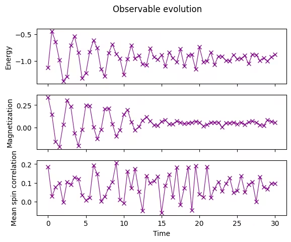
2.7 พล็อตการวิวัฒนาการเชิงเวลาของ observable

เราพล็อตค่าคาดหวังที่วัดได้เทียบกับเวลา

fig, axes = plt.subplots(3, sharex=True)
times = np.linspace(0, evolution_time, num_timesteps + 1)  # includes initial state
axes[0].plot(
    times,
    energy_array,
    label="First order",
    marker="x",
    c="darkmagenta",
    ls="-",
    lw=0.8,
)
axes[1].plot(
    times, mag_array, label="First order", marker="x", c="darkmagenta", ls="-", lw=0.8
)
axes[2].plot(
    times, corr_array, label="First order", marker="x", c="darkmagenta", ls="-", lw=0.8
)
axes[0].set_ylabel("Energy")
axes[1].set_ylabel("Magnetization")
axes[2].set_ylabel("Mean spin correlation")
axes[2].set_xlabel("Time")
fig.suptitle("Observable evolution")

Text(0.5, 0.98, 'Observable evolution')

3. แบบฝึกหัดที่ 1 ดำเนินการจำลองโดยใช้ Suzuki–Trotter อันดับที่สอง

ลองดำเนินการจำลองด้วย Suzuki–Trotter อันดับที่สองโดยอิงตามตัวอย่างของ Lie–Trotter ที่แสดงไว้ข้างต้น

Suzuki-Trotter อันดับที่สองสามารถใช้งานใน Qiskit ได้ผ่าน SuzukiTrotter class โดยใช้สูตรนี้ การแยกส่วนอันดับที่สองคือ:

$$e^{H_1+H_2} \approx e^{H_1/2}e^{H_2}e^{H_1/2}$$

3.1 สร้าง Circuit สำหรับขั้นตอนเวลาเดียว

ใช้ product_formula_st2 (SuzukiTrotter(order=2)) แล้วสร้าง Circuit สำหรับขั้นตอนเวลาเดียวโดยใช้ Suzuki–Trotter อันดับที่สอง นอกจากนี้นับจำนวน Gate และความลึกของ Circuit แล้วเปรียบเทียบกับ Lie–Trotter

# Modify the line below (Use PauliEvolutionGate)
single_step_evolution_gates_st2 = PauliEvolutionGate(
    hamiltonian, dt, synthesis=product_formula_st2
)
single_step_evolution_st2 = QuantumCircuit(n_qubits)
single_step_evolution_st2.append(
    single_step_evolution_gates_st2, single_step_evolution_st2.qubits
)
# Let us print some stats
print(
    f"""
Trotter step with second-order Suzuki-Trotter
-----------------------------
Depth: {single_step_evolution_st2.decompose(reps=3).depth()}
Gate count: {len(single_step_evolution_st2.decompose(reps=3))}
Nonlocal gate count: {single_step_evolution_st2.decompose(reps=3).num_nonlocal_gates()}
Gate breakdown: {", ".join([f"{k.upper()}: {v}" for k, v in single_step_evolution_st2.decompose(reps=3).count_ops().items()])}
"""
)
single_step_evolution_st2.decompose(reps=2).draw("mpl", fold=-1)

Trotter step with second-order Suzuki-Trotter
-----------------------------
Depth: 34
Gate count: 53
Nonlocal gate count: 20
Gate breakdown: U3: 23, CX: 20, U1: 10

3.2 ดำเนินการจำลองการวิวัฒนาการเชิงเวลา

ดำเนินการวิวัฒนาการเชิงเวลาโดยใช้ Suzuki–Trotter อันดับที่สอง

# Initiate the circuit
evolved_state = QuantumCircuit(initial_circuit.num_qubits)
# Start from the initial spin configuration
evolved_state.append(initial_circuit, evolved_state.qubits)
# Initiate Estimator (V2)
estimator = StatevectorEstimator()
# Set number of shots
shots = 10000
# Translate the precision required from the number of shots
precision = np.sqrt(1 / shots)
energy_list_st2 = []
mag_list_st2 = []
corr_list_st2 = []
# Estimate expectation values for t=0.0
job = estimator.run(
    [(evolved_state, [hamiltonian, magnetization, correlation])], precision=precision
)
# Get estimated expectation values
evs = job.result()[0].data.evs
energy_list_st2.append(evs[0])
mag_list_st2.append(evs[1])
corr_list_st2.append(evs[2])
# Start time evolution
for n in range(num_timesteps):
    # Expand the circuit to describe delta-t
    evolved_state.append(single_step_evolution_gates_st2, evolved_state.qubits)
    # Estimate expectation values at delta-t
    job = estimator.run(
        [(evolved_state, [hamiltonian, magnetization, correlation])],
        precision=precision,
    )
    # Retrieve results (expectation values)
    evs = job.result()[0].data.evs
    energy_list_st2.append(evs[0])
    mag_list_st2.append(evs[1])
    corr_list_st2.append(evs[2])
# Transform the list of expectation values (at each time step) to arrays
energy_array_st2 = np.array(energy_list_st2)
mag_array_st2 = np.array(mag_list_st2)
corr_array_st2 = np.array(corr_list_st2)

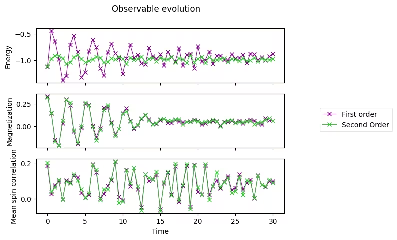
3.3 พล็อตผลลัพธ์ Suzuki–Trotter อันดับที่สอง

axes[0].plot(
    times,
    energy_array_st2,
    label="Second Order",
    marker="x",
    c="limegreen",
    ls="-",
    lw=0.8,
)
axes[1].plot(
    times,
    mag_array_st2,
    label="Second Order",
    marker="x",
    c="limegreen",
    ls="-",
    lw=0.8,
)
axes[2].plot(
    times,
    corr_array_st2,
    label="Second Order",
    marker="x",
    c="limegreen",
    ls="-",
    lw=0.8,
)

# Replace the legend
# legend.remove()
legend = fig.legend(
    *axes[0].get_legend_handles_labels(),
    bbox_to_anchor=(1.0, 0.5),
    loc="center left",
    framealpha=0.5,
)
fig

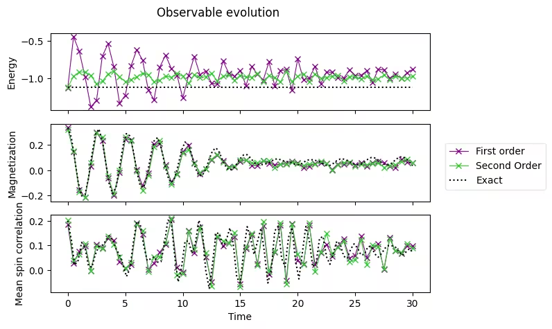
3.4 เปรียบเทียบกับผลลัพธ์ที่แม่นยำ

ข้อมูลด้านล่างคือผลลัพธ์ที่แม่นยำซึ่งคำนวณล่วงหน้าจากคอมพิวเตอร์คลาสสิก

exact_times = np.array(
    [
        0.0,
        0.3,
        0.6,
        0.8999999999999999,
        1.2,
        1.5,
        1.7999999999999998,
        2.1,
        2.4,
        2.6999999999999997,
        3.0,
        3.3,
        3.5999999999999996,
        3.9,
        4.2,
        4.5,
        4.8,
        5.1,
        5.3999999999999995,
        5.7,
        6.0,
        6.3,
        6.6,
        6.8999999999999995,
        7.199999999999999,
        7.5,
        7.8,
        8.1,
        8.4,
        8.7,
        9.0,
        9.299999999999999,
        9.6,
        9.9,
        10.2,
        10.5,
        10.799999999999999,
        11.1,
        11.4,
        11.7,
        12.0,
        12.299999999999999,
        12.6,
        12.9,
        13.2,
        13.5,
        13.799999999999999,
        14.1,
        14.399999999999999,
        14.7,
        15.0,
        15.299999999999999,
        15.6,
        15.899999999999999,
        16.2,
        16.5,
        16.8,
        17.099999999999998,
        17.4,
        17.7,
        18.0,
        18.3,
        18.599999999999998,
        18.9,
        19.2,
        19.5,
        19.8,
        20.099999999999998,
        20.4,
        20.7,
        21.0,
        21.3,
        21.599999999999998,
        21.9,
        22.2,
        22.5,
        22.8,
        23.099999999999998,
        23.4,
        23.7,
        24.0,
        24.3,
        24.599999999999998,
        24.9,
        25.2,
        25.5,
        25.8,
        26.099999999999998,
        26.4,
        26.7,
        27.0,
        27.3,
        27.599999999999998,
        27.9,
        28.2,
        28.5,
        28.799999999999997,
        29.099999999999998,
        29.4,
        29.7,
        30.0,
    ]
)
exact_energy = np.array(
    [
        -1.1184402376762155,
        -1.1184402376762157,
        -1.1184402376762157,
        -1.1184402376762148,
        -1.1184402376762153,
        -1.1184402376762155,
        -1.1184402376762148,
        -1.118440237676216,
        -1.118440237676216,
        -1.1184402376762166,
        -1.1184402376762148,
        -1.118440237676216,
        -1.1184402376762153,
        -1.1184402376762148,
        -1.118440237676217,
        -1.118440237676215,
        -1.1184402376762161,
        -1.1184402376762157,
        -1.118440237676217,
        -1.1184402376762161,
        -1.1184402376762137,
        -1.1184402376762161,
        -1.1184402376762161,
        -1.118440237676218,
        -1.1184402376762155,
        -1.1184402376762166,
        -1.1184402376762155,
        -1.1184402376762137,
        -1.1184402376762186,
        -1.1184402376762215,
        -1.1184402376762148,
        -1.118440237676216,
        -1.1184402376762166,
        -1.1184402376762148,
        -1.1184402376762121,
        -1.1184402376762166,
        -1.1184402376762181,
        -1.1184402376762137,
        -1.1184402376762148,
        -1.1184402376762193,
        -1.1184402376762108,
        -1.1184402376762144,
        -1.118440237676217,
        -1.1184402376762197,
        -1.1184402376762153,
        -1.1184402376762161,
        -1.1184402376762184,
        -1.1184402376762126,
        -1.118440237676214,
        -1.118440237676214,
        -1.1184402376762161,
        -1.118440237676212,
        -1.1184402376762164,
        -1.118440237676217,
        -1.1184402376762121,
        -1.1184402376762157,
        -1.1184402376762212,
        -1.1184402376762217,
        -1.1184402376762206,
        -1.118440237676222,
        -1.1184402376762166,
        -1.118440237676212,
        -1.1184402376762137,
        -1.11844023767622,
        -1.1184402376762206,
        -1.118440237676219,
        -1.1184402376762153,
        -1.1184402376762164,
        -1.118440237676209,
        -1.1184402376762144,
        -1.1184402376762161,
        -1.118440237676216,
        -1.1184402376762173,
        -1.118440237676214,
        -1.1184402376762093,
        -1.1184402376762184,
        -1.1184402376762126,
        -1.118440237676213,
        -1.1184402376762195,
        -1.1184402376762095,
        -1.1184402376762075,
        -1.1184402376762197,
        -1.1184402376762141,
        -1.1184402376762146,
        -1.1184402376762184,
        -1.118440237676218,
        -1.1184402376762224,
        -1.118440237676219,
        -1.118440237676218,
        -1.1184402376762206,
        -1.1184402376762168,
        -1.118440237676221,
        -1.118440237676218,
        -1.1184402376762148,
        -1.1184402376762106,
        -1.1184402376762173,
        -1.118440237676216,
        -1.118440237676216,
        -1.1184402376762113,
        -1.1184402376762275,
        -1.1184402376762195,
    ]
)
exact_magnetization = np.array(
    [
        0.3333333333333333,
        0.26316769633415005,
        0.0912947227110664,
        -0.09317712543141576,
        -0.20391854332115245,
        -0.19318196655046493,
        -0.06411527074401464,
        0.12558269854206197,
        0.28252754464640606,
        0.3264196194042506,
        0.2361586169847769,
        0.060894367906122224,
        -0.10842387093076275,
        -0.18636359582538073,
        -0.1338364343947887,
        0.020284606520827753,
        0.19151142743926025,
        0.2905341647678381,
        0.2723014646745304,
        0.15147481733047252,
        -0.008179102877790292,
        -0.1242999208732406,
        -0.1372529247781061,
        -0.04083616185958952,
        0.11066094926716476,
        0.23140661570567636,
        0.2587109403786205,
        0.1868237670027325,
        0.061201779383143744,
        -0.051391248969654205,
        -0.09843899603365061,
        -0.061297056158849166,
        0.04199010081939773,
        0.15861461430963147,
        0.22336830674799552,
        0.20179555623336537,
        0.11407111438609417,
        0.01609419104778282,
        -0.04239611796730001,
        -0.04249123521065924,
        0.008850291714888112,
        0.08780898151558082,
        0.1561486776507056,
        0.17627348772811832,
        0.13870676179652253,
        0.07205869195282538,
        0.018300003064909465,
        0.0001095640839572417,
        0.015157929316037586,
        0.05077755280969454,
        0.09245534457650838,
        0.12206907551110702,
        0.12284950557969157,
        0.09570215398601932,
        0.06294378255078983,
        0.045503313813986014,
        0.043389819499542556,
        0.046725117769796744,
        0.054956411358382404,
        0.0713814528253614,
        0.08743689703248492,
        0.08951216359166674,
        0.07878386475305985,
        0.06955669116405788,
        0.06639892435963689,
        0.05890378761746903,
        0.04541796525844558,
        0.0414221088331947,
        0.05499634106912299,
        0.07409418836014572,
        0.08371859070160165,
        0.08211623987959302,
        0.07615055161378328,
        0.06702584458783024,
        0.051891407742740085,
        0.038049378383635625,
        0.03825614149768043,
        0.054183218463525695,
        0.0753534475741016,
        0.08853147112587295,
        0.08767917178542013,
        0.07709383184439536,
        0.06308595032042386,
        0.0498812359204284,
        0.04299040064096167,
        0.04769159891460652,
        0.06483569572288776,
        0.08698035745435016,
        0.10047391641776235,
        0.09747255683203637,
        0.08098863187287358,
        0.05959496723987331,
        0.04383882265040485,
        0.04232138798062125,
        0.05720514169944535,
        0.08201306299870219,
        0.10274898262000469,
        0.10707552455080133,
        0.09210856128265357,
        0.06379922105742579,
        0.03624325103307953,
    ]
)
exact_correlation = np.array(
    [
        0.2,
        0.1247704225763532,
        0.01943938494098705,
        0.03854917181332821,
        0.11196616231067426,
        0.0906546700356683,
        0.01629373561896267,
        0.011352652889791095,
        0.0636185676540077,
        0.09543834437789013,
        0.10058518161011307,
        0.11829217731417431,
        0.1397812224038133,
        0.12316460402216707,
        0.08541383059335775,
        0.06144846844403662,
        0.020246372880505827,
        -0.02693683090021662,
        0.003919250903281282,
        0.1117419430168554,
        0.19676155181256794,
        0.18594408880783336,
        0.1002673802566004,
        0.03821525827438024,
        0.04485205090247377,
        0.05348102743040269,
        0.03160026140008638,
        0.033437649060464834,
        0.10486939975320728,
        0.20249469538955758,
        0.19735507621013149,
        0.0553097261765083,
        -0.04889114490131667,
        0.011685690974970964,
        0.11705971535823065,
        0.11681165998194759,
        0.06637091239560744,
        0.10936684225958895,
        0.20225454101061405,
        0.16284420833341812,
        -0.0025823294931362067,
        -0.0763416631752919,
        0.02985268630418397,
        0.15234468006771007,
        0.14606385406970995,
        0.0935341856492092,
        0.12325421854361143,
        0.17130422930386324,
        0.10383730044042278,
        -0.031333159406547614,
        -0.05241572078596815,
        0.07722509925347705,
        0.17642188574256007,
        0.12765340239966838,
        0.06309968945093776,
        0.11574687130499339,
        0.16978282647206913,
        0.0736143632571229,
        -0.05356602733119409,
        -0.0009649396796768892,
        0.15921620111869142,
        0.17760366431811037,
        0.04736297330213485,
        0.012122870263181897,
        0.13268065586830521,
        0.1728473023503636,
        0.03999259331072221,
        -0.036997053070222885,
        0.06951528580242439,
        0.1769169993516561,
        0.12290448295710298,
        0.012897784654866427,
        0.02859435620982225,
        0.12895847695150875,
        0.13629536955485938,
        0.05394621059822597,
        0.02298040588184324,
        0.07036499900317271,
        0.11706448623132719,
        0.10435285842074606,
        0.055721236329964965,
        0.04676334743672697,
        0.08417924910022263,
        0.10611161955304965,
        0.089304171047322,
        0.06098589533081194,
        0.06314519797488709,
        0.09431492621892917,
        0.09667836915967139,
        0.0651298357290882,
        0.05176966009147416,
        0.06727229484222669,
        0.08871788283607947,
        0.09907054249093444,
        0.09785167773502176,
        0.09277216140054353,
        0.07520999642062785,
        0.05894392248382922,
        0.07236135251622376,
        0.08608284185200156,
        0.07282922961856123,
    ]
)

axes[0].plot(exact_times, exact_energy, c="k", ls=":", label="Exact")
axes[1].plot(exact_times, exact_magnetization, c="k", ls=":", label="Exact")
axes[2].plot(exact_times, exact_correlation, c="k", ls=":", label="Exact")
# Replace the legend
legend.remove()
# Select the labels of only the first axis
legend = fig.legend(
    *axes[0].get_legend_handles_labels(),
    bbox_to_anchor=(1.0, 0.5),
    loc="center left",
    framealpha=0.5,
)
fig.tight_layout()
fig

4. รันบนฮาร์ดแวร์ควอนตัม

ต่อไปเราจะรันการจำลองการวิวัฒนาการเชิงเวลาบนฮาร์ดแวร์ควอนตัม เราจะทำงานกับปัญหาขนาดเล็กลง คือแลตทิซขนาด N=2 เราจะเปลี่ยนแปลงพารามิเตอร์ $\alpha$ เพื่อดูความแตกต่างในไดนามิกของฟังก์ชันคลื่น

4.1 ขั้นตอนที่ 1 แมปอินพุตคลาสสิกไปยังปัญหาควอนตัม

เลือกการตั้งค่าเริ่มต้นของการจำลอง:

n_qubits_2 = 2
dt_2 = 1.6
product_formula = LieTrotter(reps=1)

จากนั้นตั้งค่า Circuit เริ่มต้น:

การกำหนดค่าสปินเริ่มต้นจะเป็น "down-up"

# We prepare an initial state ↓↑ (10).
# Note that Statevector and SparsePauliOp interpret the qubits from right to left
initial_circuit_2 = QuantumCircuit(n_qubits_2)
initial_circuit_2.prepare_state("10")
# Change reps and see the difference when you decompose the circuit
initial_circuit_2.decompose(reps=1).draw("mpl")

ตอนนี้คำนวณค่าอ้างอิงโดยใช้ statevector simulator แบบ ideal

bar_width = 0.1
# initial_state = Statevector.from_label("10")
final_time = 1.6
eps = 1e-5

# We create the list of angles in radians, with a small epsilon
# the exactly longitudinal field, which would present no dynamics at all
alphas = np.linspace(-np.pi / 2 + eps, np.pi / 2 - eps, 5)

for i, alpha in enumerate(alphas):
    evolved_state_2 = QuantumCircuit(initial_circuit_2.num_qubits)
    evolved_state_2.append(initial_circuit_2, evolved_state_2.qubits)
    hamiltonian_2 = get_hamiltonian(nqubits=2, J=0.2, h=1.0, alpha=alpha)
    single_step_evolution_gates_2 = PauliEvolutionGate(
        hamiltonian_2, dt_2, synthesis=product_formula
    )
    evolved_state_2.append(single_step_evolution_gates_2, evolved_state_2.qubits)
    evolved_state_2 = Statevector(evolved_state_2)
    # Dictionary of probabilities
    amplitudes_dict = evolved_state_2.probabilities_dict()
    labels = list(amplitudes_dict.keys())
    values = list(amplitudes_dict.values())
    # Convert angle to degrees
    alpha_str = f"$\\alpha={int(np.round(alpha * 180 / np.pi))}^\\circ$"
    plt.bar(np.arange(4) + i * bar_width, values, bar_width, label=alpha_str, alpha=0.7)

plt.xticks(np.arange(4) + 2 * bar_width, labels)
plt.xlabel("Measurement")
plt.ylabel("Probability")
plt.suptitle(
    f"Measurement probabilities at $t={final_time}$, for various field angles $\\alpha$\n"
    f"Initial state: 10, Linear lattice of size $L=2$"
)
plt.legend()

<matplotlib.legend.Legend at 0x11c816590>

เราได้เตรียมระบบโดยเริ่มต้นด้วยลำดับสปิน $\downarrow\uparrow$ ซึ่งสอดคล้องกับ $\vert\psi(0)\rangle = \vert10\rangle$ หลังจากให้มันวิวัฒนาการเป็นเวลา $t=1.6$ ภายใต้สนาม transversal ($\alpha=0^\circ$) เราแทบจะวัดได้ $\uparrow\downarrow$ นั่นคือการสลับสปิน (โปรดทราบว่า label อ่านจากขวาไปซ้าย) หากสนามเป็น longitudinal ($\alpha=\pm90^\circ$) จะไม่มีการวิวัฒนาการเลย ดังนั้นเราจะวัดระบบตามที่เตรียมไว้เดิม $\downarrow\uparrow$ สำหรับมุมกลาง $\alpha=\pm45^\circ$ เราจะสามารถวัดทุกการผสมผสานด้วยความน่าจะเป็นต่างกัน โดยการสลับสปินมีโอกาสมากที่สุดที่ความน่าจะเป็น 67%

สร้าง Circuit สำหรับการทดลองบนฮาร์ดแวร์

circuit_list = []
for i, alpha in enumerate(alphas):
    evolved_state_2 = QuantumCircuit(initial_circuit_2.num_qubits)
    evolved_state_2.append(initial_circuit_2, evolved_state_2.qubits)
    hamiltonian_2 = get_hamiltonian(nqubits=2, J=0.2, h=1.0, alpha=alpha)
    single_step_evolution_gates_2 = PauliEvolutionGate(
        hamiltonian_2, dt_2, synthesis=product_formula
    )
    evolved_state_2.append(single_step_evolution_gates_2, evolved_state_2.qubits)
    evolved_state_2.measure_all()
    circuit_list.append(evolved_state_2)

4.2 ขั้นตอนที่ 2 ปรับแต่งสำหรับฮาร์ดแวร์เป้าหมาย

ระบุ Backend

service = QiskitRuntimeService()
backend = service.least_busy(operational=True, simulator=False)
backend.name

'ibm_strasbourg'

จากนั้น transpile Circuit สำหรับ Backend ที่เลือก

pm = generate_preset_pass_manager(backend=backend, optimization_level=3)
circuit_isa = pm.run(circuit_list)

ตรวจสอบ Circuit

circuit_isa[1].draw("mpl", idle_wires=False)

4.3 ขั้นตอนที่ 3 รันด้วย Qiskit Runtime primitives

Sampler (V2) ของ Qiskit ให้จำนวนครั้งของ bitstring ที่วัดได้

sampler = SamplerV2(mode=backend)
job = sampler.run(circuit_isa)
job_id = job.job_id()
print("job id:", job_id)

job id: d13pswfmya70008ek070

บันทึกผลลัพธ์

results = job.result()

4.4 ขั้นตอนที่ 4 ประมวลผลผลลัพธ์

สร้าง histogram ของ bitstring ซึ่งสอดคล้องกับการวิเคราะห์ฟังก์ชันคลื่น และเปรียบเทียบกับค่า ideal ที่แสดงไว้ข้างต้น

list_temp = ["00", "01", "10", "11"]

for i, alpha in enumerate(alphas):
    # Dictionary of probabilities
    amplitudes_dict = results[i].data.meas.get_counts()
    values = []
    for str_temp in list_temp:
        values.append(
            amplitudes_dict[str_temp] / 4096.0
        )  # divided by default number of shots
    # Convert angle to degrees
    alpha_str = f"$\\alpha={int(np.round(alpha * 180 / np.pi))}^\\circ$"
    plt.bar(np.arange(4) + i * bar_width, values, bar_width, label=alpha_str, alpha=0.7)

plt.xticks(np.arange(4) + 2 * bar_width, labels)
plt.xlabel("Measurement")
plt.ylabel("Probabilities")
plt.suptitle(
    f"Measurement probabilities at $t={final_time}$, for various field angles $\\alpha$\n"
    f"Initial state: 10, Linear lattice of size $L=2$"
)
plt.legend()

<matplotlib.legend.Legend at 0x11d7af990>

ที่นี่เราแสดงตัวอย่างการสร้าง Circuit โดยใช้ Suzuki–Trotter อันดับสูง (อันดับที่สี่) ลองสร้าง Circuit จำลองด้วย Suzuki–Trotter อันดับที่สี่โดยอิงตามตัวอย่างที่แสดงไว้ข้างต้น

Suzuki–Trotter อันดับที่สี่สามารถใช้งานใน Qiskit ได้ผ่าน SuzukiTrotter class อันดับที่สี่สามารถประเมินได้โดยใช้ความสัมพันธ์แบบ recursion ต่อไปนี้ โปรดทราบว่าอันดับของ Suzuki–Trotter แสดงด้วย "2k" ในสมการต่อไปนี้

$$\hat{U}_{ST(2k)}\left(t\right) = \left[ \hat{U}_{ST(2k-2)}\left(p_k t\right) \right]^2 \hat{U}_{ST(2k-2)}\left( (1- 4 p_k) t\right)\left[ \hat{U}_{ST(2k-2)}\left(p_k t\right) \right]^2$$ $$p_k = 1 / \left(4-4^{\frac{1}{2k-1}}\right)$$

สร้าง Circuit สำหรับขั้นตอนเวลาเดียว

ใช้ product_formula_st4 (SuzukiTrotter(order=4)) แล้วสร้าง Circuit สำหรับขั้นตอนเวลาเดียวโดยใช้ Suzuki–Trotter อันดับที่สี่ นอกจากนี้นับจำนวน Gate และความลึกของ Circuit แล้วเปรียบเทียบกับ Lie–Trotter และ Suzuki–Trotter อันดับที่สอง

# Modify the line below (Use PauliEvolutionGate)
single_step_evolution_gates_st4 = PauliEvolutionGate(
    hamiltonian, dt, synthesis=product_formula_st4
)
single_step_evolution_st4 = QuantumCircuit(n_qubits)
single_step_evolution_st4.append(
    single_step_evolution_gates_st4, single_step_evolution_st4.qubits
)
# Let us print some stats
print(
    f"""
Trotter step with second-order Suzuki-Trotter
-----------------------------
Depth: {single_step_evolution_st4.decompose(reps=3).depth()}
Gate count: {len(single_step_evolution_st4.decompose(reps=3))}
Nonlocal gate count: {single_step_evolution_st4.decompose(reps=3).num_nonlocal_gates()}
Gate breakdown: {", ".join([f"{k.upper()}: {v}" for k, v in single_step_evolution_st4.decompose(reps=3).count_ops().items()])}
"""
)
single_step_evolution_st4.decompose(reps=2).draw("mpl", fold=-1)

Trotter step with second-order Suzuki-Trotter
-----------------------------
Depth: 170
Gate count: 265
Nonlocal gate count: 100
Gate breakdown: U3: 115, CX: 100, U1: 50

# Check Qiskit version
import qiskit

qiskit.__version__

'2.0.2'