อัลกอริทึมควอนตัม: อัลกอริทึมควอนตัมแบบ Variational

หมายเหตุ

Takashi Imamichi (24 May 2024)

ดาวน์โหลด PDF ของบรรยายต้นฉบับ โปรดทราบว่าโค้ดบางส่วนอาจล้าสมัยเนื่องจากเป็นภาพ static

เวลา QPU โดยประมาณในการรันการทดลองนี้คือ 9 นาที (ทดสอบบน Eagle processor)

(notebook นี้อาจไม่สามารถ evaluate ได้ภายในเวลาที่กำหนดบน Open Plan กรุณาใช้ทรัพยากรคอมพิวเตอร์ควอนตัมอย่างประหยัด)

1. บทนำ

บทเรียนนี้ให้ภาพรวมของอัลกอริทึมแบบ hybrid quantum-classical โดยเน้นที่ variational quantum eigensolver (VQE) และ quantum approximate optimization algorithm (QAOA) เป้าหมายหลักของอัลกอริทึมเหล่านี้คือการแก้ปัญหา optimization โดยใช้ quantum circuit ที่มี parameterized quantum gate

แม้ว่าการคำนวณควอนตัมจะก้าวหน้าขึ้นมาก แต่ noise ในอุปกรณ์ควอนตัมปัจจุบันก็ยังทำให้การดึงผลลัพธ์ที่มีความหมายจาก quantum circuit ที่ลึกนั้นเป็นเรื่องยาก เพื่อแก้ปัญหานี้ VQE และ QAOA จึงใช้แนวทาง hybrid quantum-classical ซึ่งวนซ้ำการรัน quantum circuit สั้นๆ ด้วยการคำนวณควอนตัม และ optimize พารามิเตอร์ของ parameterized quantum circuit เป้าหมายด้วยการคำนวณแบบ classical

QAOA มีศักยภาพในการหาคำตอบที่ optimal สำหรับปัญหาเป้าหมายในระดับ utility ด้วยการนำเทคนิค error mitigation และ error suppression ต่างๆ มาใช้ VQE มีหลายการประยุกต์ (เช่น quantum chemistry) ที่ scale ได้น้อยกว่า แต่ก็มีแนวทาง eigenvalue ต่างๆ ที่เกิดขึ้นเพื่อเสริมและเพิ่มประสิทธิภาพ VQE รวมถึง Krylov subspace diagonalization และ sampling-based quantum diagonalization (SQD) การทำความเข้าใจ VQE เป็นก้าวแรกที่สำคัญในการทำความเข้าใจอัลกอริทึม hybrid classical-quantum ที่หลากหลายซึ่งได้ปรากฏขึ้นมา

โมดูลนี้อธิบายแนวคิดพื้นฐานและการ implement ของ VQE และ QAOA บทเรียนเพิ่มเติมจะสำรวจหัวข้อขั้นสูงและเทคนิคในการ scale up อัลกอริทึมเหล่านี้ คุณต้องมีไลบรารีต่อไปนี้ในสภาพแวดล้อมของคุณเพื่อรัน notebook นี้ หากยังไม่ได้ติดตั้ง สามารถติดตั้งได้โดยยกเลิก comment และรัน cell ต่อไปนี้

# Added by doQumentation — required packages for this notebook
!pip install -q matplotlib numpy qiskit qiskit-ibm-runtime rustworkx scipy

# % pip install 'qiskit[visualization]' qiskit-ibm-runtime

2. การคำนวณ minimum eigenvalue ของ Hamiltonian อย่างง่าย

เราจะเริ่มต้นด้วยการนำ VQE ไปใช้กับกรณีที่ง่ายมาก เพื่อดูว่ามันทำงานอย่างไร เราจะคำนวณ minimum eigenvalue ของ Pauli $Z$ matrix ด้วย VQE โดยเริ่มจากการ import package ทั่วไปบางอย่าง

import numpy as np
from qiskit.circuit import ParameterVector, QuantumCircuit
from qiskit.primitives import StatevectorEstimator, StatevectorSampler
from qiskit.quantum_info import SparsePauliOp
from scipy.optimize import minimize

ต่อไปเราจะกำหนด operator ที่สนใจและดูในรูปแบบ matrix

op = SparsePauliOp("Z")
op.to_matrix()

array([[ 1.+0.j,  0.+0.j],
       [ 0.+0.j, -1.+0.j]])

เราสามารถหา eigenvalue แบบ classical ได้ง่าย จึงตรวจสอบงานของเราได้ สิ่งนี้อาจยากขึ้นเมื่อเรา scale ไปสู่ระดับ utility ที่นี่เราใช้ numpy

# compute eigenvalues with numpy
result = np.linalg.eigh(op.to_matrix())
print("Eigenvalues:", result.eigenvalues)

Eigenvalues: [-1.  1.]

เพื่อหา eigenvalue โดยใช้ variational quantum algorithm เราสร้าง circuit ที่มี gate รับพารามิเตอร์ variational:

# define a variational form
param = ParameterVector("a", 3)
qc = QuantumCircuit(1, 1)
qc.u(param[0], param[1], param[2], 0)
qc_estimator = qc.copy()
qc.measure(0, 0)
qc.draw("mpl")

ถ้าต้องการประมาณค่า expectation value ของ operator (เช่น $Z$) ควรใช้ Estimator แต่ถ้าต้องการดูสถานะของระบบ ให้ใช้ Sampler

sampler = StatevectorSampler()
estimator = StatevectorEstimator()

เราสามารถคำนวณ count ของ bitstring 0 และ 1 ด้วยค่าพารามิเตอร์สุ่ม [1, 2, 3] โดยใช้ Sampler

# compute counts of bitstrings with random parameter values by Sampler
result = sampler.run([(qc, [1, 2, 3])]).result()
counts = result[0].data.c.get_counts()
counts

{'0': 783, '1': 241}

เราทราบว่าสามารถคำนวณ expectation value ของ Z ได้จาก $\langle Z \rangle = p_0 - p_1$ โดยมีความน่าจะเป็น $\{0: p_0, 1: p_1\}$

# compute the expectation value of Z based on the counts
(counts.get("0", 0) - counts.get("1", 0)) / sum(counts.values())

0.529296875

Circuit นี้ทำงานได้ แต่ค่าพารามิเตอร์ที่เลือกไม่ตรงกับสถานะที่มีพลังงานต่ำ (หรือ eigenvalue ต่ำ) มากนัก eigenvalue ที่ได้จึงสูงกว่า minimum อยู่มาก ผลลัพธ์ก็คล้ายกันเมื่อใช้ Estimator

โปรดทราบว่า Estimator รับ quantum circuit ที่ไม่มีการวัด

result = estimator.run([(qc_estimator, op, [1, 2, 3])]).result()
result[0].data.evs

array(0.54030231)

เราต้องค้นหาพารามิเตอร์และหาพารามิเตอร์ที่ให้ eigenvalue ต่ำที่สุด เราสร้าง function ที่รับค่าพารามิเตอร์ของ variational form และคืนค่า expectation value $\langle Z \rangle$

# define a cost function to look for the minimum eigenvalue of Z
def cost(x):
    result = sampler.run([(qc, x)]).result()
    counts = result[0].data.c.get_counts()
    expval = (counts.get("0", 0) - counts.get("1", 0)) / sum(counts.values())
    # the following line shows the trajectory of the optimization
    print(expval, counts)
    return expval

มาใช้ function minimize ของ SciPy เพื่อหา minimum eigenvalue ของ Z

# minimize the cost function with scipy's minimize
min_result = minimize(cost, [0, 0, 0], method="COBYLA", tol=1e-8)
min_result

1.0 {'0': 1024}
0.494140625 {'0': 765, '1': 259}
0.466796875 {'0': 751, '1': 273}
0.564453125 {'0': 801, '1': 223}
-0.4296875 {'1': 732, '0': 292}
-0.984375 {'1': 1016, '0': 8}
-0.8984375 {'1': 972, '0': 52}
-0.990234375 {'1': 1019, '0': 5}
-0.892578125 {'1': 969, '0': 55}
-0.986328125 {'1': 1017, '0': 7}
-0.861328125 {'1': 953, '0': 71}
-1.0 {'1': 1024}
-0.982421875 {'1': 1015, '0': 9}
-0.99609375 {'1': 1022, '0': 2}
-0.986328125 {'1': 1017, '0': 7}
-1.0 {'1': 1024}
-0.990234375 {'1': 1019, '0': 5}
-0.998046875 {'1': 1023, '0': 1}
-0.99609375 {'1': 1022, '0': 2}
-1.0 {'1': 1024}
-1.0 {'1': 1024}
-1.0 {'1': 1024}
-1.0 {'1': 1024}
-0.998046875 {'1': 1023, '0': 1}
-1.0 {'1': 1024}
-1.0 {'1': 1024}
-0.998046875 {'1': 1023, '0': 1}
-0.998046875 {'1': 1023, '0': 1}
-0.998046875 {'1': 1023, '0': 1}
-1.0 {'1': 1024}
-0.99609375 {'1': 1022, '0': 2}
-1.0 {'1': 1024}
-0.99609375 {'1': 1022, '0': 2}
-0.998046875 {'1': 1023, '0': 1}
-0.998046875 {'1': 1023, '0': 1}
-0.99609375 {'1': 1022, '0': 2}
-0.998046875 {'1': 1023, '0': 1}
-1.0 {'1': 1024}
-0.998046875 {'1': 1023, '0': 1}
-0.998046875 {'1': 1023, '0': 1}
-0.99609375 {'1': 1022, '0': 2}
-1.0 {'1': 1024}
-0.998046875 {'1': 1023, '0': 1}
-1.0 {'1': 1024}
-0.998046875 {'1': 1023, '0': 1}
-0.998046875 {'1': 1023, '0': 1}
-1.0 {'1': 1024}
-0.998046875 {'1': 1023, '0': 1}
-0.998046875 {'1': 1023, '0': 1}
-1.0 {'1': 1024}
-1.0 {'1': 1024}
-1.0 {'1': 1024}
-1.0 {'1': 1024}
-1.0 {'1': 1024}
-1.0 {'1': 1024}
-0.998046875 {'1': 1023, '0': 1}
-0.994140625 {'1': 1021, '0': 3}
-1.0 {'1': 1024}
-1.0 {'1': 1024}
-1.0 {'1': 1024}
-1.0 {'1': 1024}
-1.0 {'1': 1024}
-1.0 {'1': 1024}

message: Optimization terminated successfully.
 success: True
  status: 1
     fun: -1.0
       x: [ 3.182e+00  1.338e+00  1.664e-01]
    nfev: 63
   maxcv: 0.0

# check counts of bitstrings with the optimal parameters
result = sampler.run([(qc, min_result.x)]).result()
result[0].data.c.get_counts()

{'0': 1, '1': 1023}

2.1 แบบฝึกหัด

คำนวณ minimum eigenvalue ของ $Z \otimes Z$ ด้วย VQE

z2 = SparsePauliOp("ZZ")
print(z2)
print(z2.to_matrix())

SparsePauliOp(['ZZ'],
              coeffs=[1.+0.j])
[[ 1.+0.j  0.+0.j  0.+0.j  0.+0.j]
 [ 0.+0.j -1.+0.j  0.+0.j  0.+0.j]
 [ 0.+0.j  0.+0.j -1.+0.j  0.+0.j]
 [ 0.+0.j  0.+0.j  0.+0.j  1.+0.j]]

# compute eigenvalues with numpy

# define a variational form
# qc = ...

# compute counts of bitstrings with a random parameter values by Sampler
# result = sampler.run(...)
# result

# compute the expectation value of ZZ based on the counts

# verify the expectation value of ZZ with Estimator

# define a cost function to look for the minimum eigenvalue of ZZ
# def cost(x):
#    expval = ...
#    return expval

# minimize the cost function with scipy's minimize
# min_result = minimize(cost, [...], method="COBYLA", tol=1e-8)
# min_result

# check counts of bitstrings with the optimal parameter values
# result = sampler.run(qc, min_result.x).result()
# result

เฉลยแบบฝึกหัด

เราจะกำหนด operator ที่สนใจและดูในรูปแบบ matrix

z2 = SparsePauliOp("ZZ")
print(z2)
print(z2.to_matrix())

SparsePauliOp(['ZZ'],
              coeffs=[1.+0.j])
[[ 1.+0.j  0.+0.j  0.+0.j  0.+0.j]
 [ 0.+0.j -1.+0.j  0.+0.j  0.+0.j]
 [ 0.+0.j  0.+0.j -1.+0.j  0.+0.j]
 [ 0.+0.j  0.+0.j  0.+0.j  1.+0.j]]

เพื่อหา eigenvalue โดยใช้ variational quantum algorithm เราสร้าง circuit ที่มี gate รับพารามิเตอร์ variational:

# define a variational form
param = ParameterVector("a", 6)
qc = QuantumCircuit(2, 2)
qc.u(param[0], param[1], param[2], 0)
qc.u(param[3], param[4], param[5], 1)
qc_estimator = qc.copy()
qc.measure([0, 1], [0, 1])
qc.draw("mpl")

ถ้าต้องการประมาณค่า expectation value ของ operator (เช่น $Z \otimes Z$) เราจะใช้ Estimator แต่ถ้าต้องการดูสถานะของระบบ ให้ใช้ Sampler

sampler = StatevectorSampler()
estimator = StatevectorEstimator()

# compute counts of bitstrings with random parameter values by Sampler
result = sampler.run([(qc, [1, 2, 3, 4, 5, 6])]).result()
counts = result[0].data.c.get_counts()
counts

{'10': 661, '11': 203, '01': 47, '00': 113}

# compute the expectation value of ZZ based on the counts
(
    counts.get("00", 0)
    - counts.get("01", 0)
    - counts.get("10", 0)
    + counts.get("11", 0)
) / sum(counts.values())

-0.3828125

Circuit นี้ทำงานได้ แต่ค่าพารามิเตอร์ที่เลือกไม่ตรงกับสถานะที่มีพลังงานต่ำ (หรือ eigenvalue ต่ำ) มากนัก eigenvalue ที่ได้จึงสูงกว่า minimum อยู่มาก ผลลัพธ์ก็คล้ายกันเมื่อใช้ Estimator

# verify the expectation value of ZZ with Estimator
result = estimator.run([(qc_estimator, z2, [1, 2, 3, 4, 5, 6])]).result()
result[0].data.evs

array(-0.35316516)

เราต้องค้นหาพารามิเตอร์และหาพารามิเตอร์ที่ให้ eigenvalue ต่ำที่สุด

# define a cost function to look for the minimum eigenvalue of ZZ
def cost(x):
    result = sampler.run([(qc, x)]).result()
    counts = result[0].data.c.get_counts()
    expval = (
        counts.get("00", 0)
        - counts.get("01", 0)
        - counts.get("10", 0)
        + counts.get("11", 0)
    ) / sum(counts.values())
    print(expval, counts)
    return expval

# minimize the cost function with scipy's minimize
min_result = minimize(cost, [0, 0, 0, 0, 0, 0], method="COBYLA", tol=1e-8)
min_result

1.0 {'00': 1024}
0.578125 {'00': 808, '01': 216}
0.5234375 {'00': 780, '01': 244}
0.548828125 {'00': 793, '01': 231}
0.3515625 {'00': 637, '10': 164, '11': 55, '01': 168}
0.3359375 {'00': 638, '11': 46, '10': 174, '01': 166}
0.283203125 {'00': 602, '10': 181, '01': 186, '11': 55}
-0.087890625 {'01': 414, '00': 184, '10': 143, '11': 283}
0.236328125 {'10': 27, '11': 623, '01': 364, '00': 10}
-0.0625 {'11': 261, '01': 403, '00': 219, '10': 141}
0.248046875 {'01': 366, '11': 628, '00': 11, '10': 19}
-0.0625 {'10': 145, '11': 254, '01': 399, '00': 226}
0.228515625 {'01': 373, '11': 609, '00': 20, '10': 22}
0.0546875 {'11': 376, '10': 273, '01': 211, '00': 164}
-0.447265625 {'01': 731, '10': 10, '11': 267, '00': 16}
-0.71484375 {'01': 871, '11': 99, '00': 47, '10': 7}
-0.46484375 {'01': 741, '00': 253, '10': 9, '11': 21}
-0.87890625 {'01': 962, '00': 39, '11': 23}
-0.640625 {'00': 176, '01': 837, '11': 8, '10': 3}
-0.88671875 {'01': 966, '00': 41, '11': 17}
-0.994140625 {'01': 1021, '11': 3}
-0.91796875 {'01': 982, '11': 35, '00': 7}
-0.994140625 {'01': 1021, '11': 2, '00': 1}
-0.939453125 {'01': 993, '00': 31}
-0.990234375 {'01': 1019, '11': 5}
-0.90234375 {'01': 974, '00': 21, '11': 29}
-0.98046875 {'01': 1014, '11': 10}
-0.994140625 {'01': 1021, '00': 3}
-0.990234375 {'01': 1019, '11': 4, '00': 1}
-0.98828125 {'01': 1018, '11': 6}
-0.990234375 {'01': 1019, '11': 4, '00': 1}
-0.994140625 {'01': 1021, '11': 2, '00': 1}
-0.99609375 {'01': 1022, '11': 2}
-0.998046875 {'01': 1023, '00': 1}
-0.99609375 {'01': 1022, '00': 2}
-1.0 {'01': 1024}
-1.0 {'01': 1024}
-1.0 {'01': 1024}
-0.998046875 {'01': 1023, '11': 1}
-1.0 {'01': 1024}
-1.0 {'01': 1024}
-1.0 {'01': 1024}
-1.0 {'01': 1024}
-1.0 {'01': 1024}
-1.0 {'01': 1024}
-1.0 {'01': 1024}
-0.998046875 {'01': 1023, '00': 1}
-0.998046875 {'01': 1023, '11': 1}
-0.998046875 {'01': 1023, '00': 1}
-1.0 {'01': 1024}
-1.0 {'01': 1024}
-1.0 {'01': 1024}
-1.0 {'01': 1024}
-1.0 {'01': 1024}
-1.0 {'01': 1024}
-0.998046875 {'01': 1023, '11': 1}
-0.998046875 {'01': 1023, '11': 1}
-1.0 {'01': 1024}
-1.0 {'01': 1024}
-0.998046875 {'01': 1023, '11': 1}
-0.998046875 {'01': 1023, '11': 1}
-0.998046875 {'01': 1023, '00': 1}
-1.0 {'01': 1024}
-1.0 {'01': 1024}
-0.998046875 {'01': 1023, '00': 1}
-1.0 {'01': 1024}
-1.0 {'01': 1024}
-1.0 {'01': 1024}
-1.0 {'01': 1024}
-0.998046875 {'01': 1023, '11': 1}
-0.998046875 {'01': 1023, '11': 1}
-1.0 {'01': 1024}
-0.998046875 {'01': 1023, '11': 1}
-1.0 {'01': 1024}
-1.0 {'01': 1024}
-1.0 {'01': 1024}
-0.998046875 {'01': 1023, '11': 1}
-0.998046875 {'01': 1023, '11': 1}
-1.0 {'01': 1024}
-1.0 {'01': 1024}
-0.998046875 {'01': 1023, '11': 1}
-0.998046875 {'01': 1023, '11': 1}
-0.998046875 {'01': 1023, '00': 1}
-1.0 {'01': 1024}
-1.0 {'01': 1024}
-1.0 {'01': 1024}
-0.998046875 {'01': 1023, '11': 1}
-1.0 {'01': 1024}
-0.99609375 {'01': 1022, '00': 1, '11': 1}
-0.998046875 {'01': 1023, '11': 1}
-0.998046875 {'01': 1023, '00': 1}
-0.998046875 {'01': 1023, '11': 1}
-1.0 {'01': 1024}
-0.99609375 {'01': 1022, '11': 1, '00': 1}
-1.0 {'01': 1024}
-0.998046875 {'01': 1023, '00': 1}
-0.994140625 {'01': 1021, '00': 3}
-0.998046875 {'01': 1023, '00': 1}
-0.99609375 {'01': 1022, '11': 2}
-1.0 {'01': 1024}
-1.0 {'01': 1024}
-0.998046875 {'01': 1023, '11': 1}
-1.0 {'01': 1024}
-1.0 {'01': 1024}
-1.0 {'01': 1024}
-1.0 {'01': 1024}
-1.0 {'01': 1024}
-1.0 {'01': 1024}
-0.998046875 {'01': 1023, '11': 1}
-1.0 {'01': 1024}
-1.0 {'01': 1024}
-1.0 {'01': 1024}
-0.998046875 {'01': 1023, '11': 1}
-0.998046875 {'01': 1023, '11': 1}
-1.0 {'01': 1024}
-0.998046875 {'01': 1023, '00': 1}
-1.0 {'01': 1024}
-1.0 {'01': 1024}
-1.0 {'01': 1024}
-1.0 {'01': 1024}
-1.0 {'01': 1024}
-1.0 {'01': 1024}
-0.998046875 {'01': 1023, '11': 1}
-0.998046875 {'01': 1023, '11': 1}
-0.998046875 {'01': 1023, '11': 1}
-0.99609375 {'01': 1022, '11': 2}
-1.0 {'01': 1024}
-0.998046875 {'01': 1023, '11': 1}

message: Optimization terminated successfully.
 success: True
  status: 1
     fun: -0.998046875
       x: [ 3.167e+00  6.940e-01  1.033e+00 -2.894e-02  8.933e-01
            1.885e+00]
    nfev: 128
   maxcv: 0.0

message: Optimization terminated successfully.
 success: True
  status: 1
     fun: -0.99609375
       x: [ 3.098e+00 -5.402e-01  1.091e+00 -1.004e-02  3.615e-01
            6.913e-01]
    nfev: 115
   maxcv: 0.0

เราได้ eigenvalue ที่ใกล้เคียงกับ minimum จาก numpy มาก

# check counts of bitstrings with the optimal parameters
result = sampler.run([(qc, min_result.x)]).result()
result[0].data.c.get_counts()

{'01': 1024}

3. Quantum Optimization ด้วย Qiskit patterns

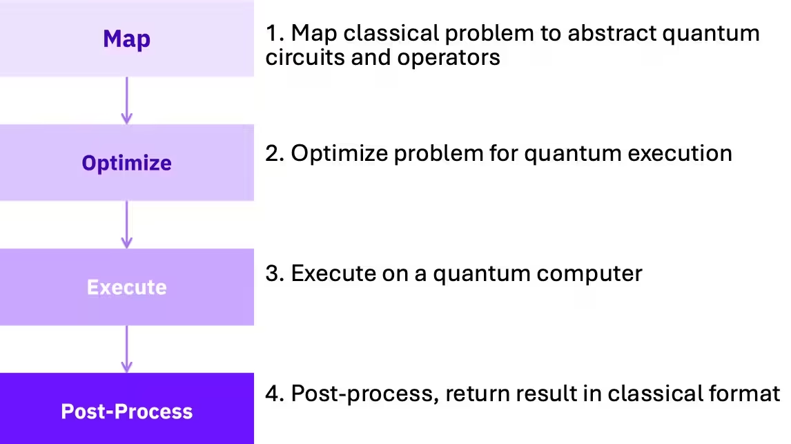
ในบทนี้เราจะเรียนรู้เกี่ยวกับ Qiskit patterns และ quantum approximate optimization Qiskit pattern คือชุดขั้นตอนที่เข้าใจง่ายและทำซ้ำได้สำหรับการ implement quantum computing workflow: เราจะนำ pattern มาประยุกต์ใช้ในบริบทของ combinatorial optimization และแสดงวิธีแก้ปัญหา Max-Cut โดยใช้ Quantum Approximate Optimization Algorithm (QAOA) ซึ่งเป็นวิธีวนซ้ำแบบ hybrid (quantum-classical)

โปรดทราบว่าส่วน QAOA นี้อ้างอิงจาก "Part 1: Small-scale QAOA" ของบทเรียน Quantum approximate optimization algorithm ดูบทเรียนดังกล่าวเพื่อเรียนรู้วิธี scale up

3.1 Qiskit pattern สำหรับ optimization (ขนาดเล็ก)

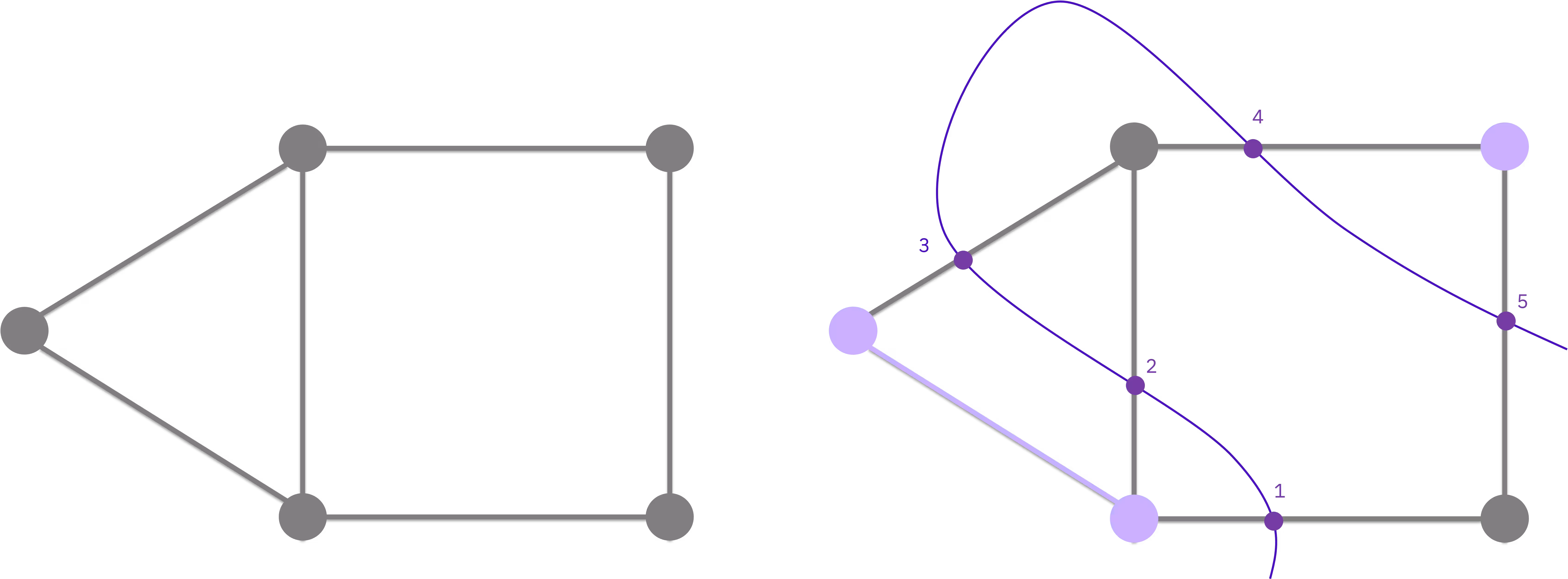
ส่วนนี้จะใช้ปัญหา Max-Cut ขนาดเล็กเพื่ออธิบายขั้นตอนที่จำเป็นในการแก้ปัญหา optimization โดยใช้คอมพิวเตอร์ควอนตัม ปัญหา Max-Cut เป็นปัญหา optimization ที่ยากในการแก้ (โดยเฉพาะเป็นปัญหา NP-hard) และมีการนำไปใช้งานหลากหลาย เช่น การจัดกลุ่ม, network science, และ statistical physics บทเรียนนี้พิจารณากราฟที่มี node เชื่อมกันด้วย edge และต้องการแบ่ง node ออกเป็นสอง set โดย "ตัด" edge เพื่อให้จำนวน edge ที่ถูกตัดมากที่สุด เพื่อให้เข้าใจบริบทก่อนที่จะ map ปัญหานี้ไปยังอัลกอริทึมควอนตัม ลองทำความเข้าใจว่าปัญหา Max-Cut กลายเป็น classical combinatorial optimization problem ได้อย่างไร โดยพิจารณาการ minimization ของ function $f(x)$

$$\min_{x\in \{0, 1\}^n}f(x),$$

โดยที่ input $x$ เป็น vector ที่แต่ละ component สอดคล้องกับ node แต่ละตัวของกราฟ จากนั้นกำหนดให้แต่ละ component เป็น $0$ หรือ $1$ (แสดงว่าถูกรวมหรือไม่รวมในการตัด) ตัวอย่างขนาดเล็กนี้ใช้กราฟที่มี $n=5$ node

เราสามารถเขียน function ของ node คู่ $i,j$ ที่บ่งบอกว่า edge $(i,j)$ ที่สอดคล้องกันอยู่ในการตัดหรือไม่ ตัวอย่างเช่น function $x_i + x_j - 2 x_i x_j$ มีค่าเป็น 1 เฉพาะเมื่อ $x_i$ หรือ $x_j$ มีค่าเป็น 1 อย่างใดอย่างหนึ่ง (ซึ่งหมายความว่า edge อยู่ในการตัด) และเป็นศูนย์ในกรณีอื่น ปัญหาการ maximize edge ในการตัดสามารถกำหนดได้ว่า

$$\max_{x\in \{0, 1\}^n} \sum_{(i,j)} x_i + x_j - 2 x_i x_j,$$

ซึ่งสามารถเขียนใหม่เป็น minimization ในรูปแบบ

$$\min_{x\in \{0, 1\}^n} \sum_{(i,j)} 2 x_i x_j - x_i - x_j.$$

minimum ของ $f(x)$ ในกรณีนี้คือเมื่อจำนวน edge ที่ถูกตัดโดย cut มีค่าสูงสุด อย่างที่เห็น ยังไม่มีส่วนไหนที่เกี่ยวกับคอมพิวเตอร์ควอนตัมเลย ต้องกำหนดปัญหานี้ใหม่ให้คอมพิวเตอร์ควอนตัมเข้าใจได้ เริ่มต้นปัญหาด้วยการสร้างกราฟที่มี $n=5$ node

import matplotlib
import matplotlib.pyplot as plt
import numpy as np
import rustworkx as rx
from rustworkx.visualization import mpl_draw

n = 5

graph = rx.PyGraph()
graph.add_nodes_from(range(1, n + 1))
edge_list = [
    (0, 1, 1.0),
    (0, 2, 1.0),
    (1, 2, 1.0),
    (1, 3, 1.0),
    (2, 4, 1.0),
    (3, 4, 1.0),
]
graph.add_edges_from(edge_list)
pos = rx.spring_layout(graph, seed=2)
mpl_draw(graph, node_size=600, pos=pos, with_labels=True, labels=str)

3.2 ขั้นตอนที่ 1: Map input แบบ classical ไปยังปัญหาควอนตัม

ขั้นตอนแรกของ pattern คือการ map ปัญหาแบบ classical (กราฟ) ไปยัง circuit และ operator ควอนตัม มีสามขั้นตอนหลักดังนี้:

1. ใช้การ reformulation ทางคณิตศาสตร์หลายขั้น เพื่อแสดงปัญหานี้ด้วย Quadratic Unconstrained Binary Optimization (QUBO)
2. เขียนปัญหา optimization ใหม่เป็น Hamiltonian ที่ ground state สอดคล้องกับคำตอบที่ minimize cost function
3. สร้าง quantum circuit ที่จะเตรียม ground state ของ Hamiltonian นี้ผ่านกระบวนการคล้าย quantum annealing

หมายเหตุ: ใน QAOA คุณต้องการ operator (Hamiltonian) ที่แสดง cost function ของ hybrid algorithm รวมถึง circuit แบบ parameterized (Ansatz) ที่แสดง quantum state ที่เป็น candidate solution ของปัญหา คุณสามารถ sample จาก candidate state เหล่านี้และประเมินด้วย cost function

กราฟ → ปัญหา optimization

ขั้นตอนแรกของการ mapping คือการเปลี่ยน notation ต่อไปนี้แสดงปัญหาใน QUBO notation:

$$\min_{x\in \{0, 1\}^n}x^T Q x,$$

โดยที่ $Q$ คือ matrix ของจำนวนจริงขนาด $n\times n$, $n$ สอดคล้องกับจำนวน node ในกราฟ, $x$ คือ vector ของ binary variable ที่แนะนำไว้ข้างต้น, และ $x^T$ หมายถึง transpose ของ vector $x$

Problem name: maxcut

Minimize
  2*x_1*x_2 + 2*x_1*x_3 + 2*x_2*x_3 + 2*x_2*x_4 + 2*x_3*x_5 + 2*x_4*x_5 - 2*x_1
  - 3*x_2 - 3*x_3 - 2*x_4 - 2*x_5

Subject to
  No constraints

  Binary variables (5)
    x_1 x_2 x_3 x_4 x_5

ปัญหา optimization → Hamiltonian

จากนั้นเราสามารถ reformulate ปัญหา QUBO เป็น Hamiltonian (ที่นี่คือ matrix ที่แสดงพลังงานของระบบ):

$$H_C=\sum_{ij}Q_{ij}Z_iZ_j + \sum_i b_iZ_i.$$

ขั้นตอน reformulation จากปัญหา QAOA ไปยัง Hamiltonian

เพื่อแสดงให้เห็นว่าปัญหา QAOA สามารถเขียนใหม่ในแบบนี้ได้อย่างไร ก่อนอื่นแทนที่ binary variable $x_i$ ด้วยตัวแปรชุดใหม่ $z_i\in\{-1, 1\}$ ผ่าน

$$x_i = \frac{1-z_i}{2}.$$

ที่นี่จะเห็นว่าถ้า $x_i$ เป็น $0$ แล้ว $z_i$ ต้องเป็น $1$ เมื่อแทน $x_i$ ด้วย $z_i$ ในปัญหา optimization ($x^TQx$) จะได้ formulation ที่เทียบเท่ากัน

$$x^TQx=\sum_{ij}Q_{ij}x_ix_j \\ =\frac{1}{4}\sum_{ij}Q_{ij}(1-z_i)(1-z_j) \\=\frac{1}{4}\sum_{ij}Q_{ij}z_iz_j-\frac{1}{4}\sum_{ij}(Q_{ij}+Q_{ji})z_i + \frac{n^2}{4}.$$

ถ้าเรากำหนด $b_i=-\sum_{j}(Q_{ij}+Q_{ji})$, ลบ prefactor, และ constant $n^2$ ออก เราจะได้สอง formulation ที่เทียบเท่ากันของปัญหา optimization เดียวกัน

$$min_{x\in\{0,1\}^n} x^TQx\Longleftrightarrow \min_{z\in\{-1,1\}^n}z^TQz + b^Tz$$

ที่นี่ $b$ ขึ้นกับ $Q$ โปรดทราบว่าในการหา $z^TQz + b^Tz$ เราละปัจจัย 1/4 และ constant offset ของ $n^2$ ซึ่งไม่มีบทบาทใน optimization

ต่อไป เพื่อให้ได้ quantum formulation ของปัญหา ส่งเสริม $z_i$ variable ไปเป็น Pauli $Z$ matrix เช่น matrix ขนาด $2\times 2$ ในรูปแบบ

$$Z_i = \begin{pmatrix}1 & 0 \\ 0 & -1\end{pmatrix}.$$

เมื่อแทน matrix เหล่านี้ในปัญหา optimization ข้างต้น จะได้ Hamiltonian ต่อไปนี้

$$H_C=\sum_{ij}Q_{ij}Z_iZ_j + \sum_i b_iZ_i.$$

นอกจากนี้ recall ว่า $Z$ matrix ถูก embed ใน computational space ของคอมพิวเตอร์ควอนตัม นั่นคือ Hilbert space ขนาด $2^n\times 2^n$ ดังนั้นควรเข้าใจ term อย่าง $Z_iZ_j$ ว่าเป็น tensor product $Z_i\otimes Z_j$ ที่ embed ใน Hilbert space ขนาด $2^n\times 2^n$ เช่น ในปัญหาที่มีห้า decision variable term $Z_1Z_3$ หมายถึง $I\otimes Z_3\otimes I\otimes Z_1\otimes I$ โดย $I$ คือ identity matrix ขนาด $2\times 2$

Hamiltonian นี้เรียกว่า cost function Hamiltonian มีคุณสมบัติว่า ground state ของมันสอดคล้องกับคำตอบที่ minimize cost function $f(x)$ ดังนั้น เพื่อแก้ปัญหา optimization คุณต้องเตรียม ground state ของ $H_C$ (หรือ state ที่มี overlap สูงกับมัน) บนคอมพิวเตอร์ควอนตัม จากนั้นการ sample จาก state นี้จะมีความน่าจะเป็นสูงที่จะได้คำตอบของ $\min~f(x)$

def build_max_cut_operator(graph: rx.PyGraph) -> tuple[SparsePauliOp, float]:
    sp_list = []
    constant = 0
    for s, t in graph.edge_list():
        w = graph.get_edge_data(s, t)
        sp_list.append(("ZZ", [s, t], w / 2))
        constant -= 1 / 2
    return SparsePauliOp.from_sparse_list(
        sp_list, num_qubits=graph.num_nodes()
    ), constant

cost_hamiltonian, constant = build_max_cut_operator(graph)
print("Cost Function Hamiltonian:", cost_hamiltonian)
print("Constant:", constant)

Cost Function Hamiltonian: SparsePauliOp(['IIIZZ', 'IIZIZ', 'IIZZI', 'IZIZI', 'ZIZII', 'ZZIII'],
              coeffs=[0.5+0.j, 0.5+0.j, 0.5+0.j, 0.5+0.j, 0.5+0.j, 0.5+0.j])
Constant: -3.0

Hamiltonian → quantum circuit

Hamiltonian $H_C$ มีนิยาม quantum ของปัญหาของคุณ ตอนนี้คุณสามารถสร้าง quantum circuit ที่จะช่วย sample คำตอบที่ดีจากคอมพิวเตอร์ควอนตัม QAOA ได้รับแรงบันดาลใจจาก quantum annealing และนำ layer ของ operator สลับกันมาใช้ใน quantum circuit

แนวคิดทั่วไปคือเริ่มต้นใน ground state ของระบบที่รู้จัก $H^{\otimes n}|0\rangle$ ข้างต้น จากนั้นนำระบบไปสู่ ground state ของ cost operator ที่สนใจ ทำได้โดยการนำ operator $\exp\{-i\gamma_k H_C\}$ และ $\exp\{-i\beta_k H_m\}$ ที่มีมุม $\gamma_1,...,\gamma_p$ และ $\beta_1,...,\beta_p~$ มาใช้

quantum circuit ที่สร้างขึ้นจะมี parameter $\gamma_i$ และ $\beta_i$ คุณจึงลองค่าต่างๆ ของ $\gamma_i$ และ $\beta_i$ และ sample จาก state ที่ได้ ในกรณีนี้เราจะลองตัวอย่างที่มี 1 QAOA layer ซึ่งมีพารามิเตอร์สองตัว: $\gamma_1$ และ $\beta_1$

from qiskit.circuit.library import QAOAAnsatz

circuit = QAOAAnsatz(cost_operator=cost_hamiltonian, reps=1)
circuit.measure_all()
circuit.draw("mpl")

circuit.decompose(reps=3).draw("mpl", fold=-1)

circuit.parameters

ParameterView([ParameterVectorElement(β[0]), ParameterVectorElement(γ[0])])

3.3 ขั้นตอนที่ 2: Optimize circuit สำหรับการรันบน quantum hardware

Circuit ข้างต้นมีชุดของ abstraction ที่มีประโยชน์ในการคิดถึงอัลกอริทึมควอนตัม แต่ไม่สามารถรันบน hardware ได้ เพื่อให้สามารถรันบน QPU ได้ circuit ต้องผ่านชุดการดำเนินการที่ประกอบเป็นขั้นตอน transpilation หรือ circuit optimization ของ pattern

ไลบรารี Qiskit มีชุด transpilation pass ที่รองรับการแปลง circuit ในรูปแบบต่างๆ ต้องตรวจสอบว่า circuit ของคุณ optimize ตามวัตถุประสงค์

Transpilation อาจเกี่ยวข้องกับหลายขั้นตอน เช่น:

• Initial mapping ของ Qubit ใน circuit (เช่น decision variable) ไปยัง physical Qubit บนอุปกรณ์
• Unrolling ของ instruction ใน quantum circuit ไปยัง hardware-native instruction ที่ Backend เข้าใจ
• Routing ของ Qubit ใดๆ ใน circuit ที่มีการ interact ไปยัง physical Qubit ที่อยู่ติดกัน
• Error suppression โดยการเพิ่ม single-qubit gate เพื่อลด noise ด้วย dynamical decoupling

ข้อมูลเพิ่มเติมเกี่ยวกับ transpilation มีอยู่ใน documentation

โค้ดต่อไปนี้แปลงและ optimize abstract circuit ให้อยู่ในรูปแบบที่พร้อมสำหรับการรันบนอุปกรณ์ที่เข้าถึงได้ผ่าน cloud โดยใช้ Qiskit IBM® Runtime service

โปรดทราบว่าคุณสามารถทดสอบโปรแกรมของคุณในเครื่อง local ด้วย "local testing mode" ก่อนที่จะส่งไปยังคอมพิวเตอร์ควอนตัมจริง ข้อมูลเพิ่มเติมเกี่ยวกับ local testing mode มีอยู่ใน documentation

from qiskit_ibm_runtime import QiskitRuntimeService
from qiskit.transpiler.preset_passmanagers import generate_preset_pass_manager

# Use a quantum device
service = QiskitRuntimeService()
backend = service.least_busy(min_num_qubits=127)
# backend = service.backend("ibm_kingston")

# You can test your programs locally with a fake backend (local testing mode)
# backend = FakeBrisbane()

print(backend)

# Create pass manager for transpilation
pm = generate_preset_pass_manager(optimization_level=3, backend=backend)

candidate_circuit = pm.run(circuit)
candidate_circuit.draw("mpl", fold=False, idle_wires=False)

service = QiskitRuntimeService(channel="ibm_quantum_platform")

<IBMBackend('ibm_strasbourg')>

3.4 ขั้นตอนที่ 3: Execute โดยใช้ Qiskit primitives

ใน QAOA workflow พารามิเตอร์ QAOA ที่ optimal จะถูกหาในลูป optimization แบบวนซ้ำ ซึ่งรันการประเมิน circuit หลายครั้งและใช้ classical optimizer เพื่อหาพารามิเตอร์ $\beta_k$ และ $\gamma_k$ ที่ optimal ลูปการ execute นี้ดำเนินการผ่านขั้นตอนต่อไปนี้:

1. กำหนดพารามิเตอร์เริ่มต้น
2. สร้าง Session ใหม่ที่มีลูป optimization และ primitive ที่ใช้ sample circuit
3. เมื่อพบชุดพารามิเตอร์ที่ optimal แล้ว ให้ execute circuit เป็นครั้งสุดท้ายเพื่อรับ distribution สุดท้ายที่จะใช้ใน post-process step

กำหนด circuit ด้วยพารามิเตอร์เริ่มต้น

เราเริ่มต้นด้วยพารามิเตอร์ที่เลือกแบบ arbitrary

initial_gamma = np.pi
initial_beta = np.pi / 2
init_params = [initial_gamma, initial_beta]

กำหนด Backend และ execution primitive

ใช้ Qiskit Runtime primitives เพื่อ interact กับ IBM® backend สอง primitive คือ Sampler และ Estimator การเลือก primitive ขึ้นอยู่กับประเภทการวัดที่ต้องการรันบนคอมพิวเตอร์ควอนตัม สำหรับการ minimize $H_C$ ให้ใช้ Estimator เนื่องจากการวัด cost function เป็นเพียง expectation value ของ $\langle H_C \rangle$

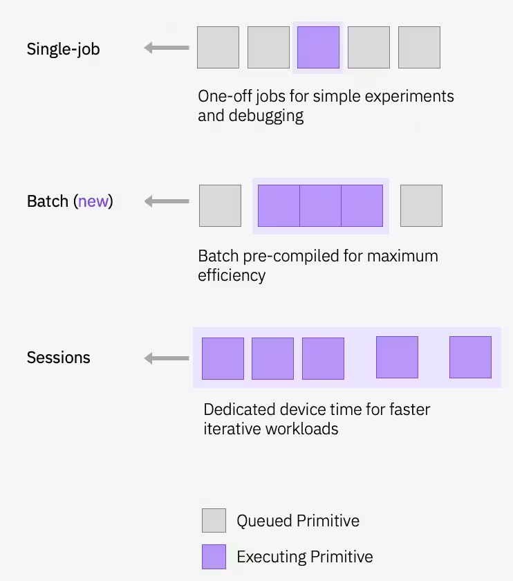
Run

Primitive มีหลาย execution mode เพื่อ schedule workload บนอุปกรณ์ควอนตัม และ QAOA workflow รันแบบวนซ้ำใน session คุณสามารถนำ sampler-based cost function ไปใส่ใน SciPy minimizing routine เพื่อหาพารามิเตอร์ที่ optimal

def cost_func_estimator(params, ansatz, hamiltonian, estimator):
    # transform the observable defined on virtual qubits to
    # an observable defined on all physical qubits
    isa_hamiltonian = hamiltonian.apply_layout(ansatz.layout)

    pub = (ansatz, isa_hamiltonian, params)
    job = estimator.run([pub])

    results = job.result()[0]
    cost = results.data.evs

    objective_func_vals.append(cost)

    return cost

from qiskit_ibm_runtime import Session, EstimatorV2
from scipy.optimize import minimize

objective_func_vals = []  # Global variable
with Session(backend=backend) as session:
    # If using qiskit-ibm-runtime<0.24.0, change `mode=` to `session=`
    estimator = EstimatorV2(mode=session)
    estimator.options.default_shots = 1000

    # Set simple error suppression/mitigation options
    estimator.options.dynamical_decoupling.enable = True
    estimator.options.dynamical_decoupling.sequence_type = "XY4"
    estimator.options.twirling.enable_gates = True
    estimator.options.twirling.num_randomizations = "auto"

    result = minimize(
        cost_func_estimator,
        init_params,
        args=(candidate_circuit, cost_hamiltonian, estimator),
        method="COBYLA",
        tol=1e-2,
    )
    print(result)

message: Optimization terminated successfully.
 success: True
  status: 1
     fun: -0.6557925874481715
       x: [ 2.873e+00  9.414e-01]
    nfev: 21
   maxcv: 0.0

Optimizer สามารถลด cost และหาพารามิเตอร์ที่ดีกว่าสำหรับ circuit ได้

plt.figure(figsize=(12, 6))
plt.plot(objective_func_vals)
plt.xlabel("Iteration")
plt.ylabel("Cost")
plt.show()

เมื่อพบพารามิเตอร์ที่ optimal สำหรับ circuit แล้ว คุณสามารถกำหนดพารามิเตอร์เหล่านี้และ sample distribution สุดท้ายที่ได้จากพารามิเตอร์ที่ optimize แล้ว นี่คือที่ที่ควรใช้ Sampler primitive เนื่องจาก probability distribution ของการวัด bitstring ตรงกับ optimal cut ของกราฟ

หมายเหตุ: หมายความว่าต้องเตรียม quantum state $\psi$ ในคอมพิวเตอร์แล้ววัดมัน การวัดจะ collapse state ไปยัง computational basis state เดียว เช่น 010101110000... ซึ่งสอดคล้องกับ candidate solution $x$ ของปัญหา optimization เดิม ($\max f(x)$ หรือ $\min f(x)$ ขึ้นกับงาน)

optimized_circuit = candidate_circuit.assign_parameters(result.x)
optimized_circuit.draw("mpl", fold=False, idle_wires=False)

from qiskit_ibm_runtime import SamplerV2

# If using qiskit-ibm-runtime<0.24.0, change `mode=` to `backend=`
sampler = SamplerV2(mode=backend)

# Set simple error suppression/mitigation options
sampler.options.dynamical_decoupling.enable = True
sampler.options.dynamical_decoupling.sequence_type = "XY4"
sampler.options.twirling.enable_gates = True
sampler.options.twirling.num_randomizations = "auto"

pub = (optimized_circuit,)
job = sampler.run([pub], shots=int(1e4))
counts_int = job.result()[0].data.meas.get_int_counts()
counts_bin = job.result()[0].data.meas.get_counts()
shots = sum(counts_int.values())
final_distribution_int = {key: val / shots for key, val in counts_int.items()}
final_distribution_bin = {key: val / shots for key, val in counts_bin.items()}
print(final_distribution_int)

{12: 0.0652, 31: 0.0089, 4: 0.0085, 13: 0.0731, 26: 0.0256, 28: 0.0246, 17: 0.0405, 25: 0.0591, 20: 0.031, 15: 0.0221, 8: 0.017, 21: 0.0371, 14: 0.0461, 16: 0.0229, 19: 0.0723, 23: 0.0199, 22: 0.0478, 18: 0.0708, 24: 0.0165, 6: 0.0525, 7: 0.0155, 5: 0.0245, 3: 0.0231, 29: 0.0121, 30: 0.0062, 10: 0.0363, 1: 0.0097, 9: 0.042, 27: 0.0094, 11: 0.0349, 0: 0.0129, 2: 0.0119}

3.5 ขั้นตอนที่ 4: Post-process และคืนผลลัพธ์ในรูปแบบ classical

ขั้นตอน post-processing แปลผลลัพธ์การ sample เพื่อคืนคำตอบสำหรับปัญหาเดิม ในกรณีนี้คุณสนใจ bitstring ที่มีความน่าจะเป็นสูงสุดเพราะมันกำหนด optimal cut ความสมมาตรในปัญหาอนุญาตให้มีคำตอบที่เป็นไปได้สี่แบบ และกระบวนการ sampling จะคืนหนึ่งในนั้นด้วยความน่าจะเป็นที่สูงกว่าเล็กน้อย แต่คุณจะเห็นในกราฟ distribution ข้างล่างว่าสี่ bitstring มีความน่าจะเป็นสูงกว่าอย่างชัดเจน

# auxiliary functions to sample most likely bitstring
def to_bitstring(integer, num_bits):
    result = np.binary_repr(integer, width=num_bits)
    return [int(digit) for digit in result]

keys = list(final_distribution_int.keys())
values = list(final_distribution_int.values())
most_likely = keys[np.argmax(np.abs(values))]
most_likely_bitstring = to_bitstring(most_likely, len(graph))
most_likely_bitstring.reverse()

print("Result bitstring:", most_likely_bitstring)

Result bitstring: [1, 0, 1, 1, 0]

import matplotlib.pyplot as plt

matplotlib.rcParams.update({"font.size": 10})
final_bits = final_distribution_bin
values = np.abs(list(final_bits.values()))
top_4_values = sorted(values, reverse=True)[:4]
positions = []
for value in top_4_values:
    positions.append(np.where(values == value)[0])
fig = plt.figure(figsize=(11, 6))
ax = fig.add_subplot(1, 1, 1)
plt.xticks(rotation=45)
plt.title("Result Distribution")
plt.xlabel("Bitstrings (reversed)")
plt.ylabel("Probability")
ax.bar(list(final_bits.keys()), list(final_bits.values()), color="tab:grey")
for p in positions:
    ax.get_children()[p[0].item()].set_color("tab:purple")
plt.show()

แสดงผล cut ที่ดีที่สุด

จาก optimal bit string คุณสามารถแสดงผล cut นี้บนกราฟเดิมได้

colors = ["tab:grey" if i == 0 else "tab:purple" for i in most_likely_bitstring]
mpl_draw(graph, node_size=600, pos=pos, with_labels=True, labels=str, node_color=colors)

และคำนวณค่าของ cut คำตอบไม่ optimal เนื่องจาก noise (ค่า cut ของคำตอบ optimal คือ 5)

from typing import Sequence

def evaluate_sample(x: Sequence[int], graph: rx.PyGraph) -> float:
    assert len(x) == len(
        list(graph.nodes())
    ), "The length of x must coincide with the number of nodes in the graph."
    return sum(
        x[u] * (1 - x[v]) + x[v] * (1 - x[u]) for u, v in list(graph.edge_list())
    )

cut_value = evaluate_sample(most_likely_bitstring, graph)
print("The value of the cut is:", cut_value)

The value of the cut is: 5

นี่คือบทสรุปของบทเรียน QAOA ขนาดเล็ก คุณจะเรียนรู้วิธีปรับ QAOA ในระดับ utility ใน "Part 2: scale it up!" ของบทเรียน Quantum approximate optimization algorithm

# Check Qiskit version
import qiskit

qiskit.__version__

'2.0.2'