ฮาร์ดแวร์

หมายเหตุ

Masao Tokunari และ Tamiya Onodera (14 มิถุนายน 2024)

คอร์สนี้อิงจากคอร์สสดที่จัดขึ้นที่มหาวิทยาลัยโตเกียว

PDF บรรยายของบทเรียนนี้แบ่งออกเป็นสองส่วน ดาวน์โหลดส่วนที่ 1 และ ดาวน์โหลดส่วนที่ 2 โปรดทราบว่าโค้ดบางส่วนอาจล้าสมัยแล้ว เนื่องจากเป็นภาพนิ่ง

1. บทนำ

บทเรียนนี้สำรวจฮาร์ดแวร์การประมวลผลเชิงควอนตัมสมัยใหม่

เราจะเริ่มต้นด้วยการตรวจสอบเวอร์ชันและนำเข้าแพ็กเกจที่เกี่ยวข้อง

# Added by doQumentation — required packages for this notebook
!pip install -q qiskit qiskit-ibm-runtime

import statistics

from qiskit_ibm_runtime import QiskitRuntimeService

2. Backend และ Target

Qiskit มี API สำหรับดึงข้อมูลทั้งแบบสถิตและแบบไดนามิกเกี่ยวกับอุปกรณ์ควอนตัม เราใช้ instance ของ Backend เพื่อเชื่อมต่อกับอุปกรณ์ ซึ่งประกอบด้วย instance ของ Target ซึ่งเป็นโมเดลเครื่องนามธรรมที่สรุปคุณสมบัติสำคัญ เช่น instruction set architecture (ISA) และคุณสมบัติหรือข้อจำกัดที่เกี่ยวข้อง มาใช้ instance ของ Backend เหล่านี้เพื่อดึงข้อมูลบางส่วนที่เห็นบนหน้า Compute resources บน IBM Quantum® Platform ก่อนอื่น เราสร้าง instance ของ Backend สำหรับอุปกรณ์ที่สนใจ ในตัวอย่างด้านล่าง เราเลือก "ibm_kyoto", "ibm_kawasaki" หรือเครื่อง Eagle ที่ว่างมากที่สุด การเข้าถึง QPU ของคุณอาจแตกต่างกัน ให้อัปเดตชื่อ Backend ตามนั้น

service = QiskitRuntimeService()
# backend = service.backend("ibm_kawasaki") # an Eagle, if you have access to ibm_kawasaki
backend = service.least_busy(
    operational=True, simulator=False, min_num_qubits=127
)  # Eagle
backend.name

'ibm_strasbourg'

เราเริ่มต้นด้วยข้อมูลพื้นฐาน (สถิต) เกี่ยวกับอุปกรณ์

print(
    f"""
{backend.name}, {backend.num_qubits} qubits
processor type = {backend.processor_type}
basis gates = {backend.basis_gates}
"""
)

ibm_strasbourg, 127 qubits
processor type = {'family': 'Eagle', 'revision': 3}
basis gates = ['ecr', 'id', 'rz', 'sx', 'x']

2.1 แบบฝึกหัด

ลองดึงข้อมูลพื้นฐานของอุปกรณ์ Heron ที่ชื่อ "ibm_strasbourg" ลองทำเองก่อน แต่มีโค้ดเพิ่มไว้ด้านล่างให้ตรวจสอบได้

a_heron = service.backend("ibm_strasbourg")  # a Heron

# your code here
print(
    f"""
{backend.name}, {a_heron.num_qubits} qubits
processor type = {a_heron.processor_type}
basis gates = {a_heron.basis_gates}
"""
)

ibm_strasbourg, 133 qubits
processor type = {'family': 'Heron', 'revision': '1'}
basis gates = ['cz', 'id', 'rz', 'sx', 'x']

2.2 Coupling map

ตอนนี้เราจะวาด coupling map ของอุปกรณ์ อย่างที่เห็น โหนดคือ Qubit ที่มีหมายเลขกำกับ ขอบแสดงคู่ที่สามารถใช้ Gate สำหรับการสร้างการพัวพัน 2 Qubit ได้โดยตรง โทโพโลยีนี้เรียกว่า "heavy-hex lattice"

# This function requires that Graphviz is installed. If you need to install Graphviz you can refer to:
# https://graphviz.org/download/#executable-packages for instructions.
try:
    fig = backend.coupling_map.draw()
except RuntimeError as ex:
    print(ex)
fig

3. คุณสมบัติของ Qubit

อุปกรณ์ Eagle มี 127 Qubit มาดูคุณสมบัติของ Qubit บางส่วนกัน

for qn in range(backend.num_qubits):
    if qn >= 5:
        break
    print(f"{qn}: {backend.qubit_properties(qn)}")

0: QubitProperties(t1=0.000183686508736532, t2=0.00023613944465408068, frequency=4832100227.116953)
1: QubitProperties(t1=0.00048794378526038294, t2=9.007098375327869e-05, frequency=4736264354.075363)
2: QubitProperties(t1=0.00021247781834456527, t2=7.81037910324034e-05, frequency=4859349851.150393)
3: QubitProperties(t1=0.0002936462084765663, t2=0.00011400214529510604, frequency=4679749549.503852)
4: QubitProperties(t1=0.00044229440258559125, t2=0.0003181648356339447, frequency=4845872064.050596)

มาคำนวณค่ามัธยฐานของเวลา T1 ของ Qubit กัน เปรียบเทียบผลลัพธ์กับค่าที่แสดงสำหรับอุปกรณ์บน IBM Quantum Platform

t1s = [backend.qubit_properties(qq).t1 for qq in range(backend.num_qubits)]
f"Median T1: {(statistics.median(t1s)*10**6):.2f} \u03bcs"

'Median T1: 285.43 μs'

3.1 แบบฝึกหัด

กรุณาคำนวณค่ามัธยฐานของเวลา T2 ของ Qubit ลองทำเองก่อน แต่มีโค้ดเพิ่มไว้ด้านล่างให้ตรวจสอบได้

# Your code here

t2s = [backend.qubit_properties(qq).t2 for qq in range(backend.num_qubits)]
f"Median T2: {(statistics.median(t2s)*10**6):.2f} \u03bcs"

'Median T2: 173.10 μs'

3.2 ข้อผิดพลาดของ Gate และการอ่านค่า

ตอนนี้เรามาดูข้อผิดพลาดของ Gate กัน เริ่มต้นด้วยการศึกษาโครงสร้างข้อมูลของ instance ของ target ซึ่งเป็น dictionary ที่มี key เป็นชื่อการดำเนินการ

target = backend.target
target.keys()

dict_keys(['measure', 'id', 'sx', 'delay', 'x', 'for_loop', 'rz', 'if_else', 'ecr', 'reset', 'switch_case'])

ค่าต่าง ๆ ก็เป็น dictionary เช่นกัน มาดูบางรายการของค่า (dictionary) สำหรับการดำเนินการ 'sx'

for i, qq in enumerate(target["sx"]):
    if i >= 5:
        break
    print(i, qq, target["sx"][qq])

0 (0,) InstructionProperties(duration=6e-08, error=0.0007401311759115297)
1 (1,) InstructionProperties(duration=6e-08, error=0.0003163759907528654)
2 (2,) InstructionProperties(duration=6e-08, error=0.0003183859004638003)
3 (3,) InstructionProperties(duration=6e-08, error=0.00042235914178831863)
4 (4,) InstructionProperties(duration=6e-08, error=0.011163151923589715)

มาทำเช่นเดียวกันสำหรับการดำเนินการ 'ecr' และ 'measure'

for i, edge in enumerate(target["ecr"]):
    if i >= 5:
        break
    print(i, edge, target["ecr"][edge])

0 (0, 14) InstructionProperties(duration=6.6e-07, error=0.01486295709788732)
1 (1, 0) InstructionProperties(duration=6.6e-07, error=0.015201590794522601)
2 (2, 1) InstructionProperties(duration=6.6e-07, error=0.00697838102630724)
3 (2, 3) InstructionProperties(duration=6.6e-07, error=0.008075067943986797)
4 (3, 4) InstructionProperties(duration=6.6e-07, error=0.0630164507876913)

for i, qq in enumerate(target["measure"]):
    if i >= 5:
        break
    print(i, qq, target["measure"][qq])

0 (0,) InstructionProperties(duration=1.6e-06, error=0.0078125)
1 (1,) InstructionProperties(duration=1.6e-06, error=0.155029296875)
2 (2,) InstructionProperties(duration=1.6e-06, error=0.057373046875)
3 (3,) InstructionProperties(duration=1.6e-06, error=0.02880859375)
4 (4,) InstructionProperties(duration=1.6e-06, error=0.01318359375)

อย่างที่เห็น ข้อผิดพลาดในการอ่านค่ามักมีขนาดใหญ่กว่าข้อผิดพลาดของการดำเนินการ 2-Qubit ซึ่งในทางกลับกันก็มีขนาดใหญ่กว่าการดำเนินการ 1-Qubit

เมื่อเข้าใจโครงสร้างข้อมูลแล้ว เราพร้อมจะคำนวณค่ามัธยฐานของข้อผิดพลาดสำหรับ Gate 'sx' และ 'ecr' เปรียบเทียบผลลัพธ์กับค่าที่แสดงสำหรับอุปกรณ์บน IBM Quantum Platform

sx_errors = [inst_prop.error for inst_prop in target["sx"].values()]
f"Median SX error: {(statistics.median(sx_errors)):.3e}"

'Median SX error: 2.277e-04'

ecr_errors = [inst_prop.error for inst_prop in target["ecr"].values()]
f"Median ECR error: {(statistics.median(ecr_errors)):.3e}"

'Median ECR error: 6.895e-03'

4. ภาคผนวก

คุณสมบัติที่นิยมใช้ของ Qiskit คือความสามารถในการแสดงผล ซึ่งรวมถึงตัวแสดงผล Circuit, ตัวแสดงผลสถานะและการกระจาย และตัวแสดงผล target คุณใช้สองอย่างแรกในสมุดโน้ต Jupyter ก่อนหน้าแล้ว มาใช้ความสามารถบางส่วนของตัวแสดงผล target กัน

from qiskit.visualization import plot_gate_map

plot_gate_map(backend, font_size=14)

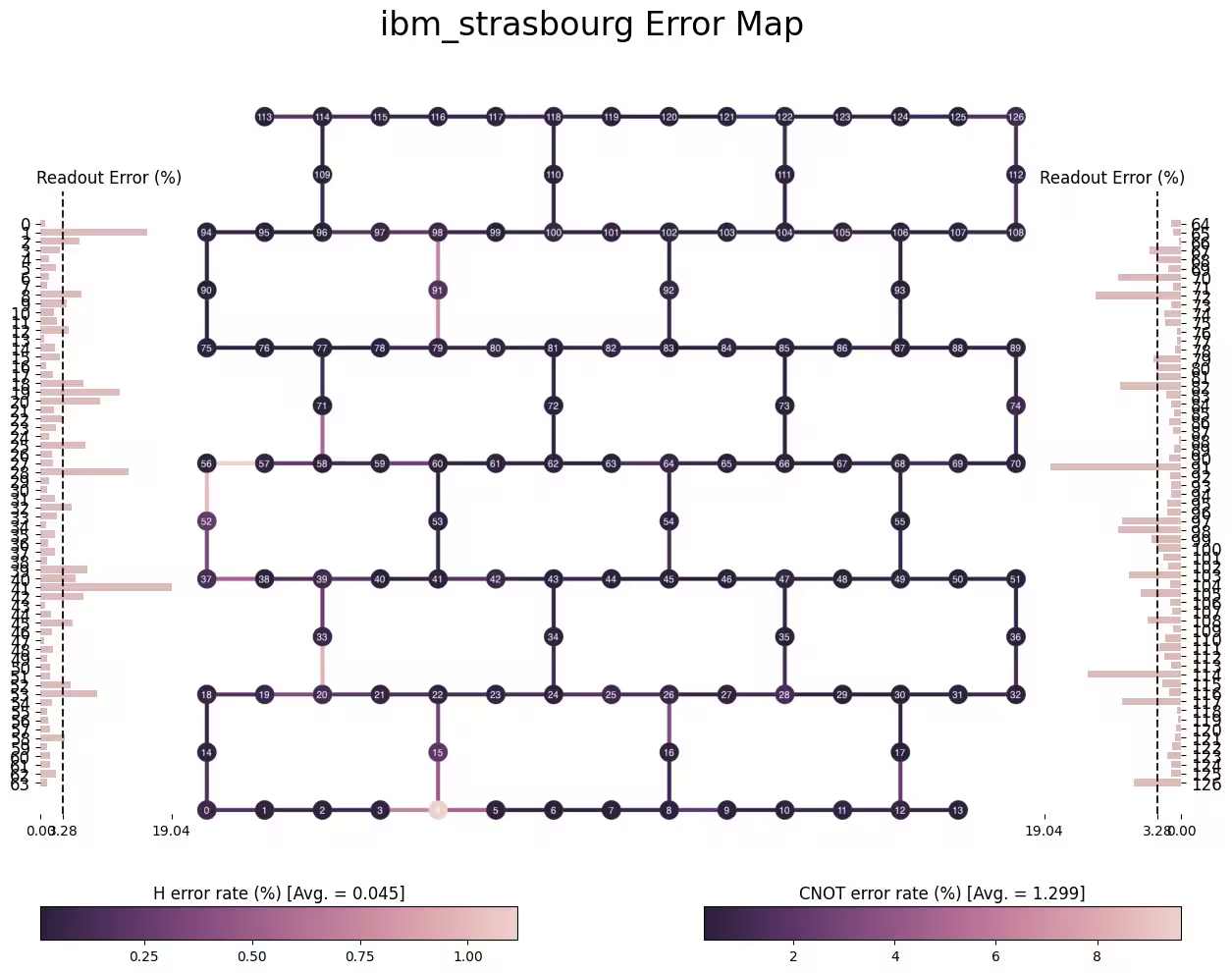
from qiskit.visualization import plot_error_map

plot_error_map(backend)

# Check Qiskit version
import qiskit

qiskit.__version__

'2.0.2'