การประมาณพลังงาน ground-state ของ Heisenberg chain ด้วย VQE

ประมาณการใช้งาน: 37 นาทีบนโปรเซสเซอร์ Heron (หมายเหตุ: นี่เป็นการประมาณเท่านั้น runtime ที่แท้จริงของคุณอาจแตกต่างออกไป)

ผลลัพธ์การเรียนรู้

หลังจากทำบทเรียนนี้เสร็จ คุณจะเข้าใจข้อมูลต่อไปนี้:

• วิธีสร้างแบบจำลอง Heisenberg spin chain เป็น quantum Hamiltonian โดยใช้ Qiskit
• วิธีใช้ตัวปรับแต่ง SPSA เพื่อประมาณพลังงาน ground-state ของระบบควอนตัม
• วิธีรัน variational workflow บนฮาร์ดแวร์ควอนตัมของ IBM® โดยใช้ Qiskit Runtime primitives และ sessions

ข้อกำหนดเบื้องต้น

แนะนำให้ทำความคุ้นเคยกับหัวข้อเหล่านี้:

• พื้นฐานสารสนเทศควอนตัม
• บทนำสู่ Qiskit patterns
• การออกแบบอัลกอริทึม variational

พื้นหลัง

Heisenberg spin chain เป็นหนึ่งในแบบจำลองที่ได้รับการศึกษามากที่สุดในฟิสิกส์สสารควบแน่นและแม่เหล็กควอนตัม มันอธิบายโครงตาข่ายหนึ่งมิติของ quantum spin ที่มีปฏิสัมพันธ์กัน โดย spin ที่อยู่ใกล้เคียงกันจะถูกเชื่อมต่อผ่านปฏิสัมพันธ์การแลกเปลี่ยน Hamiltonian สำหรับ isotropic Heisenberg model ที่มีสนามแม่เหล็กภายนอกถูกกำหนดโดย:

$H = \sum_{\langle i,j \rangle} \left( J_x X_i X_j + J_y Y_i Y_j + J_z Z_i Z_j \right) + \sum_{i} h_i Z_i,$

โดยที่ $X_i$, $Y_i$ และ $Z_i$ คือ Pauli operators ที่ทำงานบนไซต์ $i$ ผลรวม $\langle i,j \rangle$ ครอบคลุมคู่ nearest-neighbor, $J_x = J_y = J_z = 0.5$ คือค่าคงที่การเชื่อมต่อการแลกเปลี่ยน (isotropic ในบทเรียนนี้) และ $h_i$ แทนสนามแม่เหล็กภายนอกที่ขึ้นอยู่กับไซต์ ในบทเรียนนี้ ค่าสนามแม่เหล็กถูกสุ่มจากช่วง $[-1, 1]$ สังเกตว่าในการนำไปใช้งานด้านล่าง ชุดของคู่ "nearest-neighbor" ถูกกำหนดโดยการเชื่อมต่อดั้งเดิมของฮาร์ดแวร์ backend ระหว่าง $N$ qubit แรก ซึ่งอาจไม่ได้เป็น linear chain ที่เคร่งครัดขึ้นอยู่กับ topology ของอุปกรณ์

การเข้าใจพลังงาน ground-state ของ Hamiltonian นี้มีความสำคัญพื้นฐานในฟิสิกส์ ground state เก็บข้อมูลเกี่ยวกับการเปลี่ยนเฟสควอนตัม โครงสร้าง entanglement และการเรียงตัวของแม่เหล็ก ในเชิงคลาสสิก การคำนวณพลังงาน ground-state ที่แน่ชัดกลายเป็นเรื่องยากขึ้นเมื่อจำนวน spin เพิ่มขึ้น เนื่องจากมิติของ Hilbert space เพิ่มขึ้นแบบ exponential เป็น $2^N$ สำหรับ $N$ spin ทำให้เป็นผู้สมัครที่เหมาะสมสำหรับการจำลองควอนตัม

Variational Quantum Eigensolver (VQE) เป็นอัลกอริทึม hybrid quantum-classical ที่ออกแบบมาเพื่อประมาณพลังงาน ground-state ของ Hamiltonian มันทำงานโดยการเตรียม parameterized quantum state $|\psi(\theta)\rangle$ (เรียกว่า ansatz) บนคอมพิวเตอร์ควอนตัมและวัดค่าคาดหวัง $\langle \psi(\theta) | H | \psi(\theta) \rangle$ ตัวปรับแต่งคลาสสิกจะปรับพารามิเตอร์ $\theta$ แบบวนซ้ำเพื่อลดพลังงานนี้ โดยอาศัยหลักการ variational ซึ่งรับประกันว่าพลังงานที่วัดได้จะเป็นขอบเขตบนของพลังงาน ground-state ที่แท้จริงเสมอ

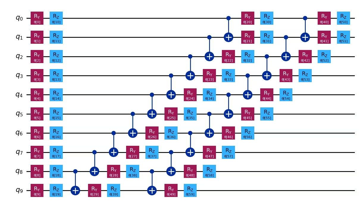
ในบทเรียนนี้ เราใช้ ansatz efficient_su2 จาก circuit library ของ Qiskit ซึ่งสร้างเลเยอร์ของการหมุน qubit เดี่ยวและ entangling gate การปรับแต่งดำเนินการโดยใช้อัลกอริทึม Simultaneous Perturbation Stochastic Approximation (SPSA) ซึ่งเหมาะสมกับฮาร์ดแวร์ควอนตัมที่มีสัญญาณรบกวน เพราะประมาณ gradient โดยใช้เพียงสองการประเมินฟังก์ชันต่อรอบโดยไม่ขึ้นอยู่กับจำนวนพารามิเตอร์

ข้อกำหนด

ก่อนเริ่มบทเรียนนี้ ตรวจสอบให้แน่ใจว่าคุณได้ติดตั้งสิ่งต่อไปนี้:

• Qiskit SDK v2.0 หรือใหม่กว่า พร้อมรองรับ visualization
• Qiskit Runtime v0.44 หรือใหม่กว่า (pip install qiskit-ibm-runtime)

การตั้งค่า

# Added by doQumentation — required packages for this notebook
!pip install -q matplotlib numpy qiskit qiskit-ibm-runtime

import numpy as np
import matplotlib.pyplot as plt
from typing import Sequence

from qiskit import QuantumCircuit
from qiskit.quantum_info import SparsePauliOp
from qiskit.primitives import BaseEstimatorV2
from qiskit.circuit.library import XGate
from qiskit.circuit.library import efficient_su2
from qiskit.transpiler import PassManager
from qiskit.transpiler.preset_passmanagers import generate_preset_pass_manager
from qiskit.transpiler.passes.scheduling import (
    ALAPScheduleAnalysis,
    PadDynamicalDecoupling,
)
from qiskit_ibm_runtime import QiskitRuntimeService, Session, EstimatorV2

def visualize_results(results):
    plt.plot(results["cost_history"], lw=2)
    plt.xlabel("Number of function evaluations")
    plt.ylabel("Energy")
    plt.show()

ตัวอย่างขนาดเล็ก

ในส่วนนี้ เราจะผ่านแต่ละขั้นตอนของ Qiskit pattern ในขนาดเล็ก โดยอธิบายส่วนประกอบสำคัญขณะที่เราสร้าง workflow

ขั้นตอนที่ 1: แมปอินพุตคลาสสิกไปยังปัญหาควอนตัม

• อินพุต: จำนวน spin
• ผลลัพธ์: Ansatz และ Hamiltonian ที่สร้างแบบจำลอง Heisenberg chain

สร้าง ansatz และ Hamiltonian ที่สร้างแบบจำลอง Heisenberg chain ที่มี 10 spin ในขั้นตอนนี้ เราจะสร้าง Heisenberg Hamiltonian ขนาด 10 spin บน coupling map ของ backend ที่ว่างที่สุด และเตรียม ansatz efficient_su2

num_spins = 10
ansatz = efficient_su2(num_qubits=num_spins, reps=2)

service = QiskitRuntimeService()
backend = service.least_busy(
    operational=True, min_num_qubits=num_spins, simulator=False
)

coupling = backend.target.build_coupling_map()
reduced_coupling = coupling.reduce(list(range(num_spins)))

edge_list = reduced_coupling.graph.edge_list()
ham_list = []

for edge in edge_list:
    ham_list.append(("ZZ", edge, 0.5))
    ham_list.append(("YY", edge, 0.5))
    ham_list.append(("XX", edge, 0.5))

for qubit in reduced_coupling.physical_qubits:
    ham_list.append(("Z", [qubit], np.random.random() * 2 - 1))

hamiltonian = SparsePauliOp.from_sparse_list(ham_list, num_qubits=num_spins)

ansatz.draw("mpl", style="iqp")

ขั้นตอนที่ 2: ปรับแต่งปัญหาสำหรับการรันบนฮาร์ดแวร์ควอนตัม

• อินพุต: Abstract circuit, observable
• ผลลัพธ์: Target circuit และ observable ที่ปรับแต่งสำหรับ QPU ที่เลือก

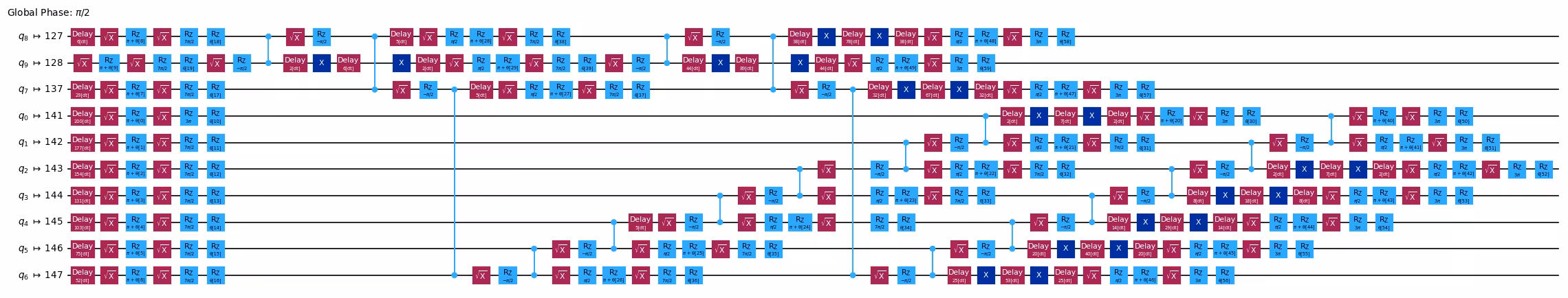
ใช้ฟังก์ชัน generate_preset_pass_manager จาก Qiskit เพื่อสร้างขั้นตอนการปรับแต่งสำหรับ Circuit ของเราโดยอัตโนมัติตาม QPU ที่เลือก เราเลือก optimization_level=3 ซึ่งให้ระดับการปรับแต่งสูงสุดของ preset pass manager นอกจากนี้เรายังเพิ่ม scheduling passes ALAPScheduleAnalysis และ PadDynamicalDecoupling เพื่อยับยั้งข้อผิดพลาด decoherence

target = backend.target
pm = generate_preset_pass_manager(optimization_level=3, target=target)
pm.scheduling = PassManager(
    [
        ALAPScheduleAnalysis(durations=target.durations()),
        PadDynamicalDecoupling(
            durations=target.durations(),
            dd_sequence=[XGate(), XGate()],
            pulse_alignment=target.pulse_alignment,
        ),
    ]
)
isa_ansatz = pm.run(ansatz)
isa_observable = hamiltonian.apply_layout(isa_ansatz.layout)
isa_ansatz.draw("mpl", scale=0.6, style="iqp", fold=-1, idle_wires=False)

ขั้นตอนที่ 3: รันโดยใช้ Qiskit primitives

• อินพุต: Target circuit และ observable
• ผลลัพธ์: ผลลัพธ์ของการปรับแต่ง

ลดพลังงาน ground-state โดยประมาณของระบบโดยปรับพารามิเตอร์ Circuit ใช้ Estimator primitive จาก Qiskit Runtime เพื่อประเมิน cost function ระหว่างการปรับแต่ง

เนื่องจากเราปรับแต่ง Circuit สำหรับ backend ในขั้นตอนที่ 2 แล้ว เราสามารถหลีกเลี่ยงการ transpile บน Runtime server ได้โดยตั้งค่า skip_transpilation=True และส่ง Circuit ที่ปรับแต่งแล้ว สำหรับการสาธิตนี้ เราจะรันบน QPU โดยใช้ primitives จาก qiskit-ibm-runtime หากต้องการรันด้วย qiskit primitives ที่ใช้ statevector ให้แทนที่บล็อกโค้ดที่ใช้ Qiskit Runtime primitives ด้วยบล็อกที่ comment ไว้

ในบทเรียนนี้เราใช้ Simultaneous Perturbation Stochastic Approximation (SPSA) ซึ่งเป็นตัวปรับแต่งแบบ gradient-based ต่อไปนี้คือบทนำสั้น ๆ เกี่ยวกับ SPSA พร้อมโค้ดสำหรับใช้งาน SPSA ด้วย Qiskit v2.0

แนะนำ SPSA

Simultaneous Perturbation Stochastic Approximation (SPSA) \[1\] เป็นอัลกอริทึมการปรับแต่งที่ประมาณเวกเตอร์ gradient ทั้งหมดโดยใช้เพียงสองการเรียกฟังก์ชันในแต่ละรอบ ให้ $f:\\mathbb{R}^p\\rightarrow \\mathbb{R}$ เป็น cost function ที่มีพารามิเตอร์ $p$ ตัวที่ต้องการปรับแต่ง และ $x_i\\in \\mathbb{R}^p$ เป็นเวกเตอร์พารามิเตอร์ที่รอบ $i^{th}$ ในการคำนวณ gradient จะสร้างเวกเตอร์สุ่ม $\\Delta_i$ ขนาด $p$ โดยแต่ละองค์ประกอบ $\\Delta_{ij}$, $\\forall$ $j\\in \\{1,2,...,p\\}$ ถูกสุ่มจาก $\\{-1, 1\\}$ แบบสม่ำเสมอ จากนั้นแต่ละองค์ประกอบของเวกเตอร์สุ่ม $\\Delta_i$ จะถูกคูณด้วยค่าเล็กน้อย $c_i$ เพื่อสร้าง random perturbation จากนั้น gradient จะถูกประมาณเป็น

$[\\nabla f(x_i)]_j \\approx \\frac{f(x_i + c_i \\Delta_i) - f(x_i - c_i \\Delta_i)}{2c_i\\Delta_{ij}}.$

โดยสัญชาตญาณแล้ว เนื่องจากมีการใช้ random perturbation ในระหว่างการประมาณ gradient จึงคาดว่าความเบี่ยงเบนเล็กน้อยในค่าที่แน่นอนของ $f$ ที่เกิดจากสัญญาณรบกวนสามารถยอมรับและรับมือได้ ในความเป็นจริง SPSA เป็นที่รู้จักเป็นพิเศษว่ามีความทนทานต่อสัญญาณรบกวน และต้องการเพียงสองการเรียกฮาร์ดแวร์ในแต่ละรอบ จึงเป็นหนึ่งในตัวปรับแต่งที่ได้รับความนิยมสูงสำหรับการใช้งานอัลกอริทึม variational

ในบทเรียนนี้ hyperparameter สำหรับรอบ $i^{th}$ คือ $a_i$ และ $c_i$ คำนวณเป็น

$a_i = \frac{a}{(A + i + 1)^\alpha} \quad \text{and} \quad c_i = \frac{c}{(i+1)^\gamma},$

โดยค่าคงที่คือ $A = 30$, $\alpha = 0.9$, $a = 0.3$, $c = 0.1$ และ $\gamma = 0.4$ ค่าเหล่านี้นำมาจาก [2] การปรับ hyperparameter อย่างเหมาะสมเป็นสิ่งจำเป็นสำหรับประสิทธิภาพที่ดีของ SPSA

def spsa(
    fun, x0, args=(), A=30, alpha=0.9, a=0.3, c=0.1, gamma=0.4, maxiter=100
):
    nparams = len(x0)
    x = np.copy(x0)

    for i in range(maxiter):
        a_i = a / (A + i + 1) ** alpha
        c_i = c / (i + 1) ** gamma
        delta_i = np.random.choice([-1, 1], nparams)

        # two hardware calls
        eval_1 = fun(x + c_i * delta_i, *args)
        eval_2 = fun(x - c_i * delta_i, *args)

        # compute the gradient and update the parameters
        grad = (eval_1 - eval_2) / (2 * c_i) * np.reciprocal(delta_i)
        x = x - a_i * grad

    return x

def cost_func(
    params: Sequence,
    ansatz: QuantumCircuit,
    hamiltonian: SparsePauliOp,
    estimator: BaseEstimatorV2,
    cost_history_dict: dict,
) -> float:
    """Ground state energy evaluation."""
    energy = (
        estimator.run([(ansatz, hamiltonian, [params])]).result()[0].data.evs
    )

    cost_history_dict["iters"] += 1
    cost_history_dict["prev_vector"] = list(params)
    cost_history_dict["cost_history"].append(float(energy[0]))

    print(
        f"Fx Iters. done: {cost_history_dict['iters']} [Current cost: {round(energy[0], 5)}]",
        end="\r",
    )

    return energy

def solve(x0, isa_ansatz, isa_observable, maxiter=150):
    cost_history_dict = {
        "prev_vector": None,
        "iters": 0,
        "cost_history": [],
        "y_min": None,
    }

    # Evaluate the problem using a QPU via Qiskit IBM Runtime
    with Session(backend=backend) as session:
        estimator = EstimatorV2(mode=session)
        estimator.skip_transpilation = True
        estimator.options.environment.job_tags = ["TUT_HSVQE"]
        x_opt = spsa(
            cost_func,
            x0=x0,
            args=(isa_ansatz, isa_observable, estimator, cost_history_dict),
            maxiter=maxiter,
        )

        y_min = cost_func(
            x_opt, isa_ansatz, isa_observable, estimator, cost_history_dict
        )

    return y_min, cost_history_dict

np.random.seed(42)
num_params = ansatz.num_parameters
params = 2 * np.pi * np.random.random(num_params)

ที่นี่เราตั้งค่า maxiter = 50 สังเกตว่าเนื่องจากแต่ละรอบต้องการสองการเรียกฟังก์ชันเพื่อคำนวณ gradient จำนวนการเรียกฟังก์ชันทั้งหมดจะเป็น $2 \\times \\text{maxiter}$ สามารถเพิ่ม maxiter เป็นค่าที่สูงขึ้นเพื่อการประมาณพลังงานที่ดีขึ้น

maxiter = 50
spsa_min, spsa_history = solve(
    params, isa_ansatz, isa_observable, maxiter=maxiter
)

Fx Iters. done: 101 [Current cost: -3.03843]

ขั้นตอนที่ 4: ประมวลผลและคืนผลลัพธ์ในรูปแบบคลาสสิกที่ต้องการ

• อินพุต: การประมาณพลังงาน ground-state ระหว่างการปรับแต่ง
• ผลลัพธ์: พลังงาน ground-state โดยประมาณ

print(f"Estimated ground state energy: {spsa_min}")

Estimated ground state energy: [-3.03842968]

results = {
    "spsa": spsa_history,
}

visualize_results(spsa_history)

ตัวอย่างฮาร์ดแวร์ขนาดใหญ่

ตัวอย่างฮาร์ดแวร์ขนาดใหญ่ไม่รวมอยู่ในบทเรียนนี้ เมื่อจำนวน qubit เพิ่มขึ้น VQE จะเผชิญกับความท้าทายอย่างมากเนื่องจากปรากฏการณ์ barren plateau: gradient ของ cost function จะลดลงแบบ exponential ตามขนาดระบบ ทำให้การปรับแต่งไม่สามารถทำได้จริงสำหรับวงจรขนาดใหญ่ รวมกับสัญญาณรบกวนจากฮาร์ดแวร์ หมายความว่าการขยาย VQE ไปยัง spin chain ขนาดใหญ่จะไม่ให้ผลลัพธ์ที่ทำซ้ำได้อย่างน่าเชื่อถือ สำหรับแนวทางที่เอาชนะข้อจำกัดเหล่านี้ ดูส่วน Next Steps ด้านล่าง

โจทย์ท้าทาย

ตอนนี้ที่คุณมีการนำ VQE ไปใช้งานสำหรับ Heisenberg chain แล้ว ลองทำสิ่งต่อไปนี้:

1. ทดลองกับความลึกของ ansatz: แก้ไขพารามิเตอร์ reps ใน efficient_su2 (ตัวอย่างเช่น ลอง reps=1 และ reps=3) ความลึกของ ansatz ส่งผลต่อพลังงาน ground-state ที่ประมาณได้และความเร็วในการลู่เข้าอย่างไร? จุดใดที่คุณสังเกตเห็นผลตอบแทนที่ลดลงหรือความไม่เสถียร?
2. ปรับ hyperparameter ของ SPSA: ปรับพารามิเตอร์ตาราง learning rate (a, c, alpha, gamma, A) และสังเกตว่ามันส่งผลต่อการลู่เข้าอย่างไร คุณสามารถหาค่าที่ลู่เข้าได้เร็วกว่าค่าเริ่มต้นที่ใช้ที่นี่ได้หรือไม่?
3. เปรียบเทียบ topology การเชื่อมต่อ: แทนที่จะใช้ coupling map ดั้งเดิมของ backend ลองสร้าง linear chain nearest-neighbor อย่างง่ายและเปรียบเทียบผลลัพธ์ การเชื่อมต่อของฮาร์ดแวร์กายภาพส่งผลต่อความลึกของวงจรที่ transpile และการประมาณพลังงานขั้นสุดท้ายอย่างไร?

อ้างอิง

[1] Spall, J. C. (2002). Implementation of the simultaneous perturbation algorithm for stochastic optimization. IEEE Transactions on Aerospace and Electronic Systems, 34(3), 817-823.

[2] Sahin, M. Emre, et al. (2025). Qiskit Machine Learning: an open-source library for quantum machine learning tasks at scale on quantum hardware and classical simulators. arXiv:2505.17756.

ขั้นตอนถัดไป

Recommendations

หากคุณสนใจงานนี้ คุณอาจสนใจเนื้อหาต่อไปนี้:

• ลอง Sample-based Quantum Diagonalization (SQD): ดังที่แสดงในบทเรียนนี้ VQE เผชิญกับความท้าทายในขนาดใหญ่เนื่องจาก barren plateau และค่าใช้จ่ายการวัดที่สูง IBM ได้พัฒนา Sample-based Quantum Diagonalization (SQD) เป็นทางเลือกที่ขยายขนาดได้มากกว่า ต่างจาก VQE ตรงที่ SQD หลีกเลี่ยงการปรับแต่ง variational ทั้งหมด แทนที่จะเป็นเช่นนั้น คอมพิวเตอร์ควอนตัมจะสร้างตัวอย่างและคอมพิวเตอร์คลาสสิกจะฉายภาพ Hamiltonian ลงบน subspace ที่ครอบคลุมโดยตัวอย่างเหล่านั้นและ diagonalize มัน ซึ่งให้ขอบเขตบนของพลังงาน ground-state ด้วยการวัดที่น้อยกว่าอย่างมีนัยสำคัญและไม่ถูกรบกวนโดย barren plateau ทำตาม บทเรียน SQD เพื่อดูแนวทางนี้ในการปฏิบัติ
• สำรวจคอร์ส Quantum Diagonalization Algorithms: เพิ่มพูนความเข้าใจเกี่ยวกับทั้ง VQE และ SQD รวมถึง trade-off ของพวกเขา ใน Quantum diagonalization algorithms บน IBM Quantum Learning