Dynamics Simulator - Qiskit Function โดย Q-CTRL Fire Opal

ดู API reference

หมายเหตุ

Qiskit Functions เป็นฟีเจอร์ทดลองที่ใช้ได้เฉพาะผู้ใช้ IBM Quantum® Premium Plan, Flex Plan และ On-Prem (ผ่าน IBM Quantum Platform API) Plan เท่านั้น อยู่ในสถานะ preview release และอาจมีการเปลี่ยนแปลง

ภาพรวม

Q-CTRL Dynamics Simulator เป็น application Qiskit Function สำหรับจำลองวิวัฒนาการตามเวลาของโมเดลควอนตัมแบบหลายวัตถุที่รองรับบนฮาร์ดแวร์ IBM Quantum แทนที่จะสร้าง quantum circuit เอง คุณระบุโมเดลทางฟิสิกส์ สถานะเริ่มต้น พารามิเตอร์การวิวัฒนาการตามเวลา และ observable ที่ต้องการวัด

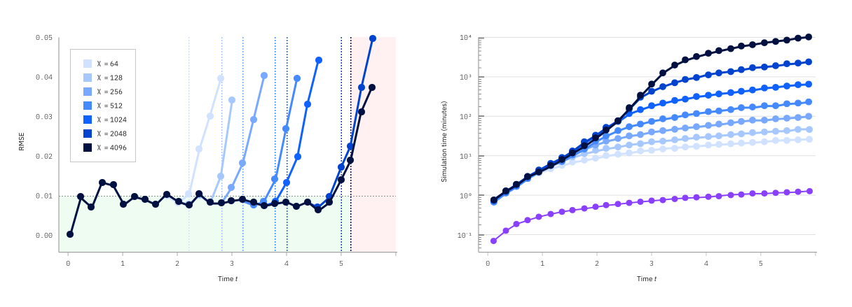
ฟังก์ชันนี้สร้างและรัน dynamic circuit ที่จำเป็น และใช้ workflow การปรับแต่งที่รับรู้ฮาร์ดแวร์และ error suppression ของ Fire Opal ผลลัพธ์คือ time trace ของค่าคาดหมายสำหรับ observable ที่คุณร้องขอ เนื่องจากฟังก์ชันใช้ error suppression โดยอัตโนมัติ คุณจึงรัน circuit ที่ความลึกระดับสถิติใหม่และยังเห็นสัญญาณที่มีความหมายได้ Dynamics Simulator ให้ความแม่นยำของคำตอบที่เทียบเท่าเครื่องมือคลาสสิกระดับ state-of-the-art ที่มีอยู่ และให้ข้อได้เปรียบด้านความเร็วที่พิสูจน์ได้

การทดสอบในโลกจริงบรรลุความสอดคล้องภายใน root mean square error (RMSE) 1% เมื่อเทียบกับการจำลอง tensor-network แบบคลาสสิกที่มีความละเอียดสูงสุด การทดสอบอิสระ จากชุมชนวิจัยยืนยันว่าคอมพิวเตอร์ควอนตัมยังคงแม่นยำแม้เกินกว่าการสาธิตเริ่มต้นของ Q-CTRL

Benchmarks

จำนวน site กำหนดจำนวน qubit ที่ต้องใช้ ส่วนจำนวน Trotter step ควบคุมความลึกของ circuit วิวัฒนาการตามเวลา แต่ละ lattice site ใช้ qubit สองตัวเพื่อแทนการครอบครองแบบ spin-up และ spin-down

workflow นี้ได้รับการสาธิตสำหรับ chain 60 site (120 qubit) ด้วย Trotter step 30 ขั้น และสำหรับ chain 31 site (62 qubit) ด้วย Trotter step 90 ขั้น ตารางด้านล่างแสดงทรัพยากรของ circuit และเวลารันบน QPU จาก การทดลองที่รายงาน ซึ่งทำบนอุปกรณ์ IBM® Heron r3 (ibm_boston) ด้วย 20,000 shot ต่อ circuit

ขนาดระบบ	Trotter step	ความลึก two-qubit	จำนวน two-qubit gate	เวลา QPU	เวลา QPU เมื่อใช้ REM + DR
10 site (20 qubit)	30	152	1,457	2m 46s	4m 25s
10 site (20 qubit)	60	302	2,897	5m 36s	8m 42s
10 site (20 qubit)	90	452	4,337	8m 46s	13m 26s
31 site (62 qubit)	30	152	4,649	2m 46s	4m 25s
31 site (62 qubit)	60	302	9,239	5m 36s	8m 42s
31 site (62 qubit)	90	452	13,829	8m 46s	13m 26s
60 site (120 qubit)	30	152	9,057	2m 46s	4m 25s

สำหรับจำนวน Trotter step ที่คงที่ ความลึกของ circuit และเวลา QPU ที่รายงานยังคงเท่าเดิมในทุกขนาดระบบที่ทดสอบ ขณะที่จำนวน two-qubit gate เพิ่มขึ้น การเพิ่มจำนวน step ทำให้ circuit ลึกขึ้นและต้องใช้เวลา QPU มากขึ้น

ในที่นี้ เวลา QPU คือเวลารันบนฮาร์ดแวร์สะสมสำหรับ circuit จำลองหลัก คอลัมน์สุดท้ายยังรวมเวลา QPU สำหรับการระบุลักษณะ noise ที่ใช้ใน readout error mitigation (REM) และ decay recovery (DR) ด้วย คู่มือนี้ใช้ตัวอย่าง Fermi-Hubbard หนึ่งมิติขนาดเล็กเพื่อแสดง workflow ทั้งหมดตั้งแต่การนิยามโมเดลจนถึงการพล็อตพลวัตที่วัดได้

คำอธิบายฟังก์ชัน

พลวัตควอนตัมอธิบายว่าระบบควอนตัมเปลี่ยนแปลงอย่างไรตามเวลา การศึกษาวิวัฒนาการนี้ช่วยให้คุณเข้าใจว่าอนุภาคเคลื่อนที่อย่างไร สหสัมพันธ์พัฒนาอย่างไร และระบบตอบสนองต่อการเปลี่ยนแปลงของสถานะหรือ Hamiltonian อย่างไร

โมเดล Fermi-Hubbard อธิบายเฟอร์มิออนที่เคลื่อนที่ระหว่าง lattice site และมีอันตรกิริยาต่อกันเมื่ออยู่ใน site เดียวกัน การแข่งขันระหว่าง hopping และอันตรกิริยาทำให้เป็นโมเดลที่มีประโยชน์สำหรับศึกษาอิเล็กตรอนที่มีสหสัมพันธ์รุนแรง วิวัฒนาการตามเวลาของมันเผยให้เห็นว่า spin และประจุแพร่กระจายอย่างไร และระบบที่เริ่มต้นเป็นระเบียบคลายตัวอย่างไร

โมเดล

Dynamics Simulator รองรับ chain Fermi-Hubbard หนึ่งมิติที่มีขอบเขตเปิด สำหรับ chain ที่มี $L$ site Hamiltonian ถูกนิยามดังนี้:

$$H = -\sum_{i=0}^{L-2}\sum_{\sigma\in\{\uparrow,\downarrow\}} t_{h,i} \left( c^\dagger_{i\sigma}c_{i+1,\sigma} + c^\dagger_{i+1,\sigma}c_{i\sigma} \right) +\sum_{i=0}^{L-1}U_i n_{i\uparrow}n_{i\downarrow} -\sum_{i=0}^{L-1}\sum_{\sigma\in\{\uparrow,\downarrow\}} \mu_i n_{i\sigma}.$$

ในที่นี้ $c^\dagger_{i\sigma}$ และ $c_{i\sigma}$ สร้างและทำลายเฟอร์มิออนที่มี spin $\sigma$ ที่ site $i$ ตัวดำเนินการจำนวน $n_{i\sigma}=c^\dagger_{i\sigma}c_{i\sigma}$ วัดการครอบครองของ spin orbital นั้น

อินพุตของโมเดลระบุสัมประสิทธิ์ต่อไปนี้:

• hopping_amplitude: $t_{h,i}$ ซึ่งควบคุม hopping ระหว่าง site ที่อยู่ติดกัน $i$ และ $i+1$

• on_site_interaction: $U_i$ อันตรกิริยาระหว่างเฟอร์มิออน spin-up และ spin-down ที่อยู่ใน site เดียวกัน

• chemical_potential: $\mu_i$ ศักย์เคมีเฉพาะที่ ซึ่งเข้าสู่ Hamiltonian ด้วยเครื่องหมายลบ

ระบุค่า scalar เพื่อใช้สัมประสิทธิ์เดียวกันตลอด chain หรือระบุ list เพื่อกำหนดสัมประสิทธิ์สำหรับแต่ละ bond หรือ site

ในหน่วยที่ $\hbar=1$ สถานะเริ่มต้นวิวัฒนาการดังนี้:

$$|\psi(t)\rangle=e^{-iHt}|\psi(0)\rangle.$$

ฟังก์ชันประเมินค่าคาดหมายของ observable ที่คุณระบุ ณ เวลาจำลองที่ต่อเนื่องกัน

Workflow

workflow ของฟังก์ชันประกอบด้วยขั้นตอนต่อไปนี้:

1. Algorithmic synthesis: ฟังก์ชันใช้ Hamiltonian และการตั้งค่าเวลาจำลองเพื่อสร้างลำดับ Trotter-Suzuki ที่ปรับให้เหมาะสม ซึ่งลดความลึกของ circuit ขณะที่คำนึงถึงความแม่นยำของการจำลอง

2. Hardware-aware mapping: ฟังก์ชัน map และ route circuit โดยใช้การเชื่อมต่อของ qubit และลักษณะข้อผิดพลาดของ IBM Quantum backend ที่เลือก

3. Physical-layer error suppression: Fire Opal ใช้ dynamical decoupling และการแก้ไขระดับ pulse เพื่อลด noise จากสภาพแวดล้อมและ crosstalk ระหว่างการรันบนฮาร์ดแวร์

ฟังก์ชันจัดการขั้นตอนเหล่านี้โดยอัตโนมัติและส่งคืนค่าคาดหมายของ observable ที่ร้องขอตามเวลา

คุณนิยามปัญหาทางฟิสิกส์และการตั้งค่าการจำลองผ่านอินพุตของฟังก์ชัน อินเทอร์เฟซปัจจุบันรองรับวิวัฒนาการตามเวลาแบบ Trotter โดย time_step กำหนดระยะเวลาของแต่ละ step และ step_count กำหนดจำนวน step

สำหรับรายละเอียดเพิ่มเติม ดู Fire Opal dynamics simulator overview และ simulate_dynamics API reference

เริ่มต้นใช้งาน

ดูข้อมูลการเข้าถึง Qiskit Function นี้ได้ใน Qiskit Functions Catalog

คู่มือนี้แสดงวิธีโหลด Dynamics Simulator และจำลอง chain Fermi-Hubbard สี่ site โค้ดต่อไปนี้สมมติว่าคุณบันทึก IBM Quantum Platform API key และ instance CRN ไว้ใน environment บนเครื่องของคุณแล้ว

สำหรับการตั้งค่าบัญชีและวิธีติดตั้ง client ดู Get started with Qiskit Functions

# Added by doQumentation — installs the packages this notebook needs if they are missing
import importlib.util

_needed = {"matplotlib": "matplotlib", "numpy": "numpy", "qctrlvisualizer": "qctrlvisualizer", "qiskit_ibm_catalog": "qiskit-ibm-catalog"}
_missing = [pip for module, pip in _needed.items()
            if importlib.util.find_spec(module) is None]
# One at a time, so a package that fails to install does not block the others
for _pip in _missing:
    %pip install -q {_pip}
if not _missing:
    print("\u2713 All required packages are installed")

from qiskit_ibm_catalog import QiskitFunctionsCatalog

catalog = QiskitFunctionsCatalog(channel="ibm_quantum_platform")

# Access the Q-CTRL Dynamics Simulator Qiskit Function.
sim_qf = catalog.load("q-ctrl/dynamics-simulator")

# Check the list of backends you have access to
catalog.backends()

[<IBMBackend('ibm_boston')>,
 <IBMBackend('ibm_fez')>,
 <IBMBackend('ibm_kingston')>,
 <IBMBackend('ibm_marrakesh')>,
 <IBMBackend('ibm_miami')>,
 <IBMBackend('ibm_phoenix')>,
 <IBMBackend('ibm_pittsburgh')>]

# Select the backend you want to use
backend = catalog.backend("ibm_phoenix")

ตัวอย่าง: จำลอง chain Fermi-Hubbard สี่ site

พิจารณา chain Fermi-Hubbard หนึ่งมิติสี่ site ที่มี hopping amplitude $t_h=1$ ไม่มี on-site interaction และศักย์เคมีเป็นศูนย์ เฟอร์มิออน spin-up หนึ่งตัวเริ่มที่ site 0 และวิวัฒนาการไปตาม chain

ปัญหาขนาดเล็กนี้ช่วยให้โฟกัสที่ workflow ของ Dynamics Simulator:

1. นิยามโมเดลและการจำลอง

2. นิยามสถานะเริ่มต้นและ observable

3. ส่ง Qiskit Function job

4. ดึงค่าคาดหมาย

5. พล็อตพลวัต

1. กำหนดปัญหา

site_count = 4

model = {
    "hopping_amplitude": 1.0,
    "on_site_interaction": 0.0,
    "chemical_potential": 0.0,
}

simulation = {
    "time_step": 0.2,
    "step_count": 8,
}

initial_state = "eeeu"

observables = [
    {
        "operators": [[["Nup", site]]],
        "coefficients": [1.0],
    }
    for site in range(site_count)
]

shot_count = 2048

รายการ observable วัดการครอบครองของสปินอัพ

$$\langle n_{i\uparrow} \rangle$$

ที่แต่ละไซต์ โดย observable จะถูกส่งคืนตามลำดับเดียวกับที่ระบุเข้าไป

2. รันการจำลองพลวัต

ส่งปัญหาผ่าน Qiskit Function โดย Qiskit Functions Catalog จะจัดการการยืนยันตัวตนของ IBM Quantum ให้ ดังนั้นคุณไม่ต้องส่งข้อมูลรับรองของ Fire Opal หรือผู้ให้บริการฮาร์ดแวร์แยกต่างหากไปที่ sim_qf.run()

job = sim_qf.run(
    model=model,
    simulation=simulation,
    observables=observables,
    initial_state=initial_state,
    shots=shot_count,
    backend_name=backend.name,
)

print(job.job_id, job.status())

68202fad-6919-425d-8fd2-c1c649cd15b1 DONE

ออบเจกต์ที่ส่งคืนคือ Qiskit Function job คุณเก็บ job ID ไว้เพื่อดึงข้อมูลหรือตรวจสอบเวิร์กโหลดนี้ภายหลังได้

3. ดึงผลลัพธ์

result = job.result()

print("Result keys:", sorted(result.keys()))
print("Warnings:", result.get("warnings", []))

Result keys: ['metadata', 'observable_expectation_values', 'observables', 'warnings']
Warnings: []

แปลงค่าคาดหวังของ observable เป็นอาร์เรย์ NumPy โดยแต่ละแถวตรงกับ observable หนึ่งตัว และแต่ละคอลัมน์ตรงกับเวลาจำลองที่บันทึกไว้หนึ่งค่า เริ่มจาก $t=0$ ในตัวอย่างนี้ทั้งสี่แถวคือการครอบครองของสปินอัพที่ไซต์ 0 ถึง 3

import numpy as np

expectation_values = np.asarray(
    result["observable_expectation_values"],
    dtype=float,
)

print("Expectation-value array shape:", expectation_values.shape)

Expectation-value array shape: (4, 9)

4. แสดงภาพพลวัต

สถานะเริ่มต้นมีเฟอร์มิออนสปินอัพหนึ่งตัวและไม่มีเฟอร์มิออนสปินดาวน์เลย ดังนั้นวิวัฒนาการของมันจึงอยู่ในปริภูมิย่อยอนุภาคเดี่ยว ซึ่งสถานะฐานทั้งสี่ตรงกับกรณีที่เฟอร์มิออนอยู่ที่ไซต์ 0, 1, 2 และ 3

ในปริภูมิย่อยนี้ Hamiltonian เชื่อมไซต์ที่อยู่ติดกันด้วยแอมพลิจูดการกระโดด $-t_h$ สำหรับพารามิเตอร์ที่ใช้ในที่นี้

$$H_{\mathrm{1p}} = -t_h \begin{pmatrix} 0 & 1 & 0 & 0 \\ 1 & 0 & 1 & 0 \\ 0 & 1 & 0 & 1 \\ 0 & 0 & 1 & 0 \end{pmatrix}.$$

ทำ diagonalize เมทริกซ์นี้ด้วย NumPy แล้วให้สถานะเริ่มต้นวิวัฒน์ที่เวลาเดียวกับที่ Dynamics Simulator ส่งคืนมา กำลังสองของขนาดแอมพลิจูดของแต่ละสถานะให้การครอบครองของสปินอัพของไซต์นั้น

การคำนวณนี้ให้วิวัฒนาการของ Hamiltonian ที่แม่นยำ ความแตกต่างระหว่างค่าประมาณจากฮาร์ดแวร์กับค่าอ้างอิงนี้อาจมาจากขั้น Trotter ที่มีขนาดจำกัด สถิติการวัด และข้อผิดพลาดที่เหลืออยู่ของฮาร์ดแวร์

times = np.arange(expectation_values.shape[1]) * simulation["time_step"]

# This reference is specific to a single spin-up fermion.
if (
    len(initial_state) != site_count
    or initial_state.count("u") != 1
    or initial_state.count("e") != site_count - 1
):
    raise ValueError(
        "This reference requires one spin-up fermion and otherwise empty sites."
    )

# Build the Hamiltonian in the single-particle subspace.
hamiltonian = -model["hopping_amplitude"] * (
    np.eye(site_count, k=1) + np.eye(site_count, k=-1)
)
hamiltonian -= model["chemical_potential"] * np.eye(site_count)

# The rightmost character of initial_state corresponds to site 0.
initial_amplitudes = np.zeros(site_count, dtype=complex)
initial_site = initial_state[::-1].index("u")
initial_amplitudes[initial_site] = 1.0

# Evolve the initial state in the Hamiltonian eigenbasis.
energies, eigenvectors = np.linalg.eigh(hamiltonian)
initial_coefficients = eigenvectors.conj().T @ initial_amplitudes

phases = np.exp(-1j * np.outer(energies, times))
states = eigenvectors @ (initial_coefficients[:, None] * phases)

ideal_expectation_values = np.abs(states) ** 2

พล็อตหนึ่งแผงต่อหนึ่งไซต์ เส้นทึบแสดงค่าอ้างอิงที่แม่นยำ ณ เวลาที่บันทึกไว้ และเครื่องหมายแสดงค่าประมาณจากฮาร์ดแวร์ที่ Dynamics Simulator ส่งคืนมา

import matplotlib.pyplot as plt
import qctrlvisualizer as qv
from qctrlvisualizer import QCTRL_STYLE_COLORS as colors

plt.style.use(qv.get_qctrl_style())

fig, ax = plt.subplots(figsize=(10, 6))

for site in range(len(expectation_values)):
    site_color = colors[site % len(colors)]

    ax.plot(
        times,
        ideal_expectation_values[site],
        color=site_color,
        linewidth=2,
        label=f"Site {site}: exact reference",
    )

    ax.plot(
        times,
        expectation_values[site],
        color=site_color,
        linestyle="--",
        linewidth=1.5,
        marker="o",
        markersize=5,
        label=f"Site {site}: hardware estimate",
    )

ax.set_xlim(times[0], times[-1])
ax.set_ylim(-0.05, 1.05)

ax.set_xlabel(r"Time (units of $\hbar/t_h$)")
ax.set_ylabel(r"$\langle n_{i\uparrow} \rangle$")
ax.set_title("Spin-up occupation dynamics")

ax.legend(
    ncol=2,
    fontsize=10,
    loc="best",
)

fig.tight_layout()
plt.show()

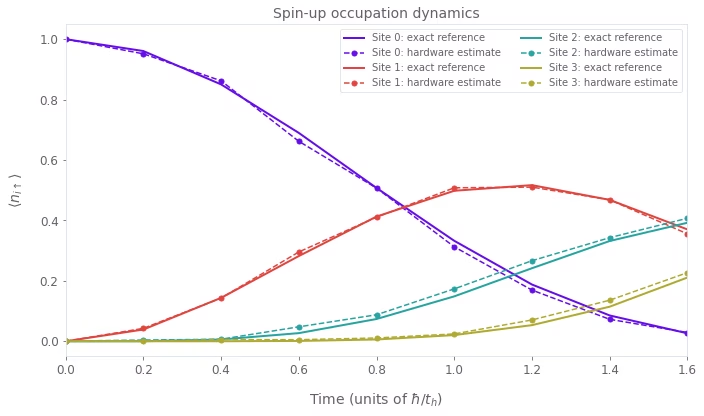
ที่ $t=0$ การครอบครองของสปินอัพที่แม่นยำคือ 1 ที่ไซต์ 0 และ 0 ที่ไซต์อื่น เมื่อระบบวิวัฒน์ไป การกระโดดจะกระจายความน่าจะเป็นของอนุภาคไปตามโซ่ การครอบครองของไซต์ 1 เพิ่มขึ้นก่อน ตามด้วยการครอบครองที่เพิ่มขึ้นที่ไซต์ 2 และ 3 สำหรับพารามิเตอร์ในตัวอย่างนี้ เวลาสุดท้ายที่บันทึกไว้คือ $t=1.6$ การครอบครองที่แม่นยำของไซต์ 0 ถึง 3 อยู่ที่ประมาณ 0.026, 0.370, 0.392 และ 0.211 ตามลำดับ

การครอบครองที่แม่นยำเป็นไปตามสมการต่อไปนี้ทุกเวลา ซึ่งสะท้อนการอนุรักษ์จำนวนอนุภาค:

$$\sum_{i=0}^{3}\langle n_{i\uparrow}(t)\rangle=1$$

การครอบครองของแต่ละไซต์อาจเพิ่มขึ้นและลดลงได้ขณะที่อนุภาควิวัฒน์ไปตามโซ่จำกัด

ดึงข้อความแสดงข้อผิดพลาด

หากเวิร์กโหลดเข้าสู่สถานะ ERROR ให้เรียก job.result() เพื่อดึงข้อความแสดงข้อผิดพลาด คุณยังตรวจสอบบันทึกของ function ได้ด้วย หากมีให้ใช้

print(job.status())

if job.status() == "ERROR":
    print(job.result())
    print(job.logs())

DONE

ปัญหาการตรวจสอบอินพุตที่พบบ่อยได้แก่ โมเดลหรือวิธีจำลองที่ไม่รองรับ สตริงสถานะเริ่มต้นที่ยาวเกินไป พจน์และสัมประสิทธิ์ของ observable ที่ไม่ตรงกัน หรือ observable ที่อ้างอิงไซต์นอกสตริงสถานะเริ่มต้น

รับความช่วยเหลือ

หากมีคำถามเกี่ยวกับ Dynamics Simulator หรือพฤติกรรมของ Fire Opal ดูเอกสารของ Q-CTRL หรือติดต่อ Q-CTRL

สำหรับการยืนยันตัวตนของ Qiskit Functions การจัดการ job หรือการเข้าถึง IBM Quantum Platform ดูเอกสารของ Qiskit Functions

ขั้นตอนถัดไป

คำแนะนำ

• ดูเอกสารอ้างอิง API ของ simulate_dynamics สำหรับคำนิยามของโมเดล การจำลอง observable เอาต์พุต และการตรวจสอบความถูกต้อง
• ลองทำบทเรียนพลวัตของสปินและประจุในโมเดล Fermi-Hubbard
• อ่านภาพรวมของ Fire Opal dynamics simulator เพื่อดูรายละเอียดเพิ่มเติมเกี่ยวกับ Trotterization การแมปที่คำนึงถึงฮาร์ดแวร์ และการลดทอนข้อผิดพลาดของ Fire Opal
• ปรับพารามิเตอร์ของโมเดล สถานะเริ่มต้น ขนาดขั้นเวลา จำนวนขั้น และ observable เพื่อศึกษาปัญหาพลวัต Fermi-Hubbard หนึ่งมิติแบบอื่น