พลวัตของสปินและประจุในโมเดล Fermi-Hubbard

ประมาณการการใช้งาน: 5 นาทีบนตัวประมวลผล Heron r3 (หมายเหตุ: เป็นเพียงการประมาณ เวลารันจริงของคุณอาจต่างออกไป)

ความเป็นมา

โมเดล Fermi-Hubbard อธิบายอิเล็กตรอนที่กระโดดบนแลตทิซ โดยมีบทลงโทษด้านพลังงานเมื่อมีอิเล็กตรอนสองตัวอยู่ที่ไซต์เดียวกัน บนสายโซ่หนึ่งมิติที่มี $L$ ไซต์และขอบเปิด Hamiltonian ถูกกำหนดดังนี้

$$H = -\sum_{i=0}^{L-2} \sum_{\sigma \in \{\uparrow,\downarrow\}} t_{h,i} \left( c^\dagger_{i\sigma} c_{i+1,\sigma} + \mathrm{h.c.} \right) + \sum_{i=0}^{L-1} U_i\, n_{i\uparrow} n_{i\downarrow} - \sum_{i=0}^{L-1} \sum_\sigma \mu_i\, n_{i\sigma},$$

โดยที่ $c^\dagger_{i\sigma}$ สร้างเฟอร์มิออนที่มีสปิน $\sigma$ บนไซต์ $i$ และ $n_{i\sigma} = c^\dagger_{i\sigma} c_{i\sigma}$ นับจำนวนของมัน สามพจน์คือแอมพลิจูดการกระโดด $t_{h,i}$ บนพันธะระหว่างไซต์ $i$ และ $i+1$ อันตรกิริยาบนไซต์ $U_i$ และศักย์เคมี $\mu_i$ บทเรียนนี้วัดพลังงานในหน่วย $t_h$ และเวลาในหน่วย $1/t_h$

พลวัตเรียลไทม์ของโมเดลนี้คำนวณด้วยวิธีคลาสสิกได้ยาก Exact diagonalization หยุดอยู่ราว $L \lesssim 14$ ไซต์ และหลัง quench เอนโทรปีของ entanglement ของ tensor-network solver จะโตเชิงเส้นตามเวลา ทำให้ bond dimension ที่ต้องใช้เพื่อความแม่นยำคงที่โตแบบเอกซ์โพเนนเชียล

ในหนึ่งมิติ การกระตุ้นพื้นฐานคือ spinon ซึ่งมีสปินแต่ไม่มีประจุ และ holon ซึ่งมีประจุแต่ไม่มีสปิน ทั้งสองแพร่ด้วยความเร็วต่างกัน ดังนั้นการรบกวนเฉพาะที่จึงแยกเป็น front เร็วและ front ช้า ปรากฏการณ์นี้เรียกว่า spin-charge separation และบทเรียนนี้วัดมัน [1]

บทเรียนนี้ใช้ Dynamics Simulator Qiskit Function ซึ่งรับ Hamiltonian สถานะเริ่มต้น ตาราง Trotter และรายการ observable แล้วส่งคืนค่าคาดหมาย มันจัดการ Jordan-Wigner mapping, Trotterization, ผัง qubit และการกดทอน error ภายในเอง จึงไม่มี circuit ให้สร้างหรือ transpile ในบทเรียนนี้

สิ่งที่ต้องมี

ก่อนเริ่มบทเรียนนี้ ตรวจสอบให้แน่ใจว่าคุณติดตั้งแพ็กเกจต่อไปนี้แล้ว

• Qiskit SDK v2.3.0 ขึ้นไป (pip install qiskit)

• Qiskit Runtime v0.50.0 ขึ้นไป (pip install qiskit-ibm-runtime)

• Qiskit Functions Catalog v0.21.0 ขึ้นไป (pip install qiskit-ibm-catalog)

• NumPy v2.5.1 ขึ้นไป (pip install numpy)

• Matplotlib v3.10.3 ขึ้นไป (pip install matplotlib)

• Q-CTRL Visualizer v11.0.0 ขึ้นไป (pip install qctrl-visualizer)

การตั้งค่า

ก่อนอื่น ยืนยันตัวตนด้วย IBM Quantum API key ของคุณ จากนั้นเลือก Qiskit Function ดังนี้ (โค้ดนี้สมมติว่าคุณบันทึกบัญชีของคุณไว้ในสภาพแวดล้อมในเครื่องแล้ว)

# Added by doQumentation — installs the packages this notebook needs if they are missing
import importlib.util

_needed = {"matplotlib": "matplotlib", "numpy": "numpy", "qctrlvisualizer": "qctrlvisualizer", "qiskit_ibm_catalog": "qiskit-ibm-catalog", "qiskit_ibm_runtime": "qiskit-ibm-runtime", "scipy": "scipy"}
_missing = [pip for module, pip in _needed.items()
            if importlib.util.find_spec(module) is None]
# One at a time, so a package that fails to install does not block the others
for _pip in _missing:
    %pip install -q {_pip}
if not _missing:
    print("\u2713 All required packages are installed")

import numpy as np
import matplotlib.pyplot as plt
from scipy import stats
from qiskit_ibm_catalog import QiskitFunctionsCatalog
from qiskit_ibm_runtime import QiskitRuntimeService
import qctrlvisualizer as qv

plt.style.use(qv.get_qctrl_style())

catalog = QiskitFunctionsCatalog(channel="ibm_quantum_platform")

# Access Function
sim_qf = catalog.load("q-ctrl/dynamics-simulator")

ขั้นตอนที่ 1: แมปอินพุตคลาสสิกไปเป็นปัญหาควอนตัม

กำหนด Hamiltonian

ฟังก์ชันรับโมเดลเป็น dictionary ที่มีสามคีย์ แต่ละคีย์รับได้ทั้ง float ค่าเดียวซึ่งใช้เท่ากันตลอดสายโซ่ หรือลิสต์ที่ระบุค่าทีละไซต์ ลิสต์มี $L-1$ รายการสำหรับ hopping_amplitude เพราะสายโซ่เปิดมีพันธะน้อยกว่าไซต์หนึ่งพันธะ และมี $L$ รายการสำหรับ on_site_interaction และ chemical_potential

บทเรียนนี้ใช้สายโซ่สม่ำเสมอ 31 ไซต์ที่มีอันตรกิริยาแบบผลัก $U/t_h = 8$ ศักย์เคมีที่สม่ำเสมอให้เพียงเฟสรวมเมื่อจำนวนอนุภาคคงที่ ตัวอย่างนี้จึงตั้งเป็นศูนย์ ศักย์เคมีมีความสำคัญเมื่อมันเปลี่ยนไปตามไซต์เท่านั้น เช่น เพื่อเพิ่ม disorder หรือสิ่งเจือปนเดี่ยว

site_count = 31
hopping_amplitude = 1.0
on_site_interaction = 8.0
chemical_potential = 0.0

model = {
    "hopping_amplitude": [hopping_amplitude] * (site_count - 1),
    "on_site_interaction": [on_site_interaction] * site_count,
    "chemical_potential": [chemical_potential] * site_count,
}

print(
    f"{site_count} sites, {2 * site_count} qubits, U/t_h = {on_site_interaction:.0f}"
)

31 sites, 62 qubits, U/t_h = 8

ตั้งค่าตาราง Trotter

dictionary simulation เก็บขนาดก้าวเวลา ($\Delta t$) และจำนวนก้าว Trotter โดยเวลาวิวัฒนาการรวมคือผลคูณของทั้งสอง ก้าวที่ใหญ่กว่าไปถึงเวลาที่ไกลกว่าที่ความลึก circuit คงที่ แต่เกิด Trotter error มากขึ้น ซึ่งโตตาม $U$ เพราะพจน์ของ Hamiltonian สลับที่กันได้น้อยลง การศึกษาบนฮาร์ดแวร์ที่ตีพิมพ์ใช้ $\Delta t = 0.15$ สำหรับ $U/t_h = 8$ [2] และบทเรียนนี้ใช้ค่าเดียวกัน ความลึก circuit โตเชิงเส้นตามจำนวนก้าวและไม่ขึ้นกับ $L$ เลย

time_step = 0.15
step_count = 30

simulation = {"time_step": time_step, "step_count": step_count}

print(
    f"Total evolution time: t = {time_step * step_count:.2f} (units of 1/t_h)"
)

Total evolution time: t = 4.50 (units of 1/t_h)

เตรียมสถานะเริ่มต้น

แต่ละไซต์มีสปินออร์บิทัลสองตัว ดังนั้นสายโซ่ $L$ ไซต์ใช้ $2L$ qubit สถานะเริ่มต้นเป็นสตริงการครอบครองแบบ Fock ที่มีหนึ่งตัวอักษรต่อไซต์

$$\begin{aligned} \texttt{empty (e)} &\longleftrightarrow \left(n_{i,\uparrow}, n_{i,\downarrow}\right) = (0,0), \\ \texttt{up (u)} &\longleftrightarrow \left(n_{i,\uparrow}, n_{i,\downarrow}\right) = (1,0), \\ \texttt{down (d)} &\longleftrightarrow \left(n_{i,\uparrow}, n_{i,\downarrow}\right) = (0,1), \\ \texttt{both (b)} &\longleftrightarrow \left(n_{i,\uparrow}, n_{i,\downarrow}\right) = (1,1). \end{aligned}$$

สตริงถูกอ่านโดยเริ่มจากไซต์ที่มีนัยสำคัญน้อยที่สุด ดังนั้นตัวอักษรขวาสุดคือไซต์ 0 และดัชนีไซต์จริงของตัวอักษรที่ $k$ นับจากซ้ายคือ $i = L - 1 - k$ สตริง udud จึงหมายความว่าไซต์ 0 คือ d, ไซต์ 1 คือ u, ไซต์ 2 คือ d และไซต์ 3 คือ u

ถัดไป เตรียมสถานะ Néel แบบเติมครึ่ง สลับ u และ d โดยแทนไซต์กลางด้วยที่ว่าง ที่ว่างนี้คือการรบกวนที่เราติดตามการแผ่ขยายของมัน

vacancy_site = site_count // 2

# Build in increasing site order, then reverse: the leftmost character of the
# string is the highest site index.
site_occupations = [
    "u" if site % 2 == 0 else "d" for site in range(site_count)
]
site_occupations[vacancy_site] = "e"
initial_state = "".join(reversed(site_occupations))

print(f"Vacancy at site {vacancy_site}")
print(initial_state)

Vacancy at site 15
udududududududueudududududududu

สร้าง observable

observable แต่ละตัวเป็น dictionary ที่แทนผลรวมถ่วงน้ำหนักของผลคูณของตัวดำเนินการการครอบครอง

$$O = \sum_{\alpha} c_{\alpha} \prod_{(\sigma, j) \in T_{\alpha}} n_{j,\sigma}.$$

ทุกรายการของ operators คือหนึ่งพจน์ $T_{\alpha}$ เขียนเป็นลิสต์ของคู่ [name, site] ที่คูณกัน และรายการที่ตรงกันของ coefficients คือน้ำหนักของมัน ชื่อทั้งสองคือ "Nup" สำหรับ $n_{j,\uparrow}$ และ "Ndn" สำหรับ $n_{j,\downarrow}$ observable จุดเดียวหนึ่งตัว $n_{3,\uparrow}$ เขียนได้ดังนี้

{"operators": [[["Nup", 3]]], "coefficients": [1.0]}

เซลล์ถัดไปพิมพ์ชุดอินพุตที่สมบูรณ์เล็กที่สุดที่ฟังก์ชันรับได้ ซึ่งมีประโยชน์เป็นแบบอ้างอิงรูปร่างขณะอ่านโค้ดต่อจากนี้

minimal_inputs = {
    "model": {
        "hopping_amplitude": 1.0,
        "on_site_interaction": [2.0, 2.5],
        "chemical_potential": 0.5,
    },
    "simulation": {"step_count": 5, "time_step": 0.1},
    "observables": [{"operators": [[["Nup", 0]]], "coefficients": [1.0]}],
    "initial_state": "ud",
    "shots": 4096,
}

for key, value in minimal_inputs.items():
    print(f"{key}: {value}")

model: {'hopping_amplitude': 1.0, 'on_site_interaction': [2.0, 2.5], 'chemical_potential': 0.5}
simulation: {'step_count': 5, 'time_step': 0.1}
observables: [{'operators': [[['Nup', 0]]], 'coefficients': [1.0]}]
initial_state: ud
shots: 4096

ต้องใช้ observable สามกลุ่ม ความหนาแน่นประจุ $n_i = n_{i\uparrow} + n_{i\downarrow}$ และสปินเฉพาะที่ $S^z_i = (n_{i\uparrow} - n_{i\downarrow})/2$ ต่างเป็นผลรวมสองพจน์บนตัวดำเนินการชุดเดียวกัน ต่างกันที่สัมประสิทธิ์เท่านั้น ตัวสัมพันธ์สปิน $S^z_i S^z_{i_*}$ ระหว่างไซต์ $i$ และไซต์ที่ว่างขยายเป็นพจน์สองจุดสี่พจน์ที่มีสัมประสิทธิ์ $\pm 1/4$

ตัวดำเนินการการครอบครองสลับที่กันได้ ดังนั้นลำดับของตัวประกอบภายในพจน์ไม่มีผล แต่ลำดับของลิสต์ observables กำหนดลำดับของค่าที่ส่งคืน โค้ดบันทึกดัชนีของแต่ละกลุ่มขณะสร้างลิสต์ ตัวสัมพันธ์ข้ามไซต์ที่ว่างไป เพราะตรงนั้นผลคูณจะซ้ำตัวประกอบ

observables = []
charge_indices = []
spin_indices = []
correlator_indices = []

# Charge density: n_i = n_{i,up} + n_{i,down}
for site in range(site_count):
    charge_indices.append(len(observables))
    observables.append(
        {
            "operators": [[["Nup", site]], [["Ndn", site]]],
            "coefficients": [1.0, 1.0],
        }
    )

# Local spin: S^z_i = (n_{i,up} - n_{i,down}) / 2
for site in range(site_count):
    spin_indices.append(len(observables))
    observables.append(
        {
            "operators": [[["Nup", site]], [["Ndn", site]]],
            "coefficients": [0.5, -0.5],
        }
    )

# Spin correlator: S^z_i S^z_{i_*}, expanded into four two-point terms.
correlator_sites = [
    site for site in range(site_count) if site != vacancy_site
]
for site in correlator_sites:
    correlator_indices.append(len(observables))
    observables.append(
        {
            "operators": [
                [["Nup", site], ["Nup", vacancy_site]],
                [["Nup", site], ["Ndn", vacancy_site]],
                [["Ndn", site], ["Nup", vacancy_site]],
                [["Ndn", site], ["Ndn", vacancy_site]],
            ],
            "coefficients": [0.25, -0.25, -0.25, 0.25],
        }
    )

print(f"{len(observables)} observables")
print("Example correlator:", observables[correlator_indices[0]])

92 observables
Example correlator: {'operators': [[['Nup', 0], ['Nup', 15]], [['Nup', 0], ['Ndn', 15]], [['Ndn', 0], ['Nup', 15]], [['Ndn', 0], ['Ndn', 15]]], 'coefficients': [0.25, -0.25, -0.25, 0.25]}

ขั้นตอนที่ 2: ปรับปัญหาให้เหมาะกับการรันบนฮาร์ดแวร์ควอนตัม

บทเรียนนี้ไม่มีขั้นตอน transpilation ฟังก์ชันทำขั้นตอนต่อไปนี้ภายใน [2] และคุณกำหนดค่าจาก notebook ไม่ได้

• แมปโหมดเฟอร์มิออนไปยัง qubit ตามลำดับที่เลือกเพื่อให้น้ำหนัก Pauli ต่ำบนแลตทิซ heavy-hex

• ใช้ fermionic SWAP network เพื่อให้ทุกพจน์การกระโดดกลายเป็นการหมุนสอง qubit

• ฝังสายโซ่ไปตามเส้นทางที่หลีกเลี่ยง qubit ที่อ่อน

• ใช้ dynamical decoupling และ Pauli twirling ระหว่างการคอมไพล์

คุณเลือก backend และจำนวน shot ฟังก์ชันรับชื่อ backend เป็นสตริง บทเรียนนี้จึงเลือกอุปกรณ์ที่ว่างที่สุดซึ่งใหญ่พอสำหรับสายโซ่ แล้วส่งชื่อของมัน

สัญญาณที่เล็กที่สุดที่คุณต้องแยกแยะเป็นตัวกำหนดจำนวน shot ตัวติดตามประจุได้แอมพลิจูดใกล้ $0.15$ แต่ตัวติดตามสปินแบบ connected มีค่าสูงสุดราว $0.04$ เล็กกว่าประมาณสี่เท่า การศึกษาที่ตีพิมพ์จึงใช้ 20,000 shot ต่อ circuit [2]

service = QiskitRuntimeService()
backend = service.backend("ibm_boston")
backend_name = backend.name
shot_count = 20_000

print(f"{backend_name}, {shot_count} shots per circuit")

ibm_boston, 20000 shots per circuit

ขั้นตอนที่ 3: รันโดยใช้ Qiskit primitives

ถัดไป ส่งการจำลอง run ส่งคืน job handle ทันทีโดยไม่บล็อก

job = sim_qf.run(
    model=model,
    simulation=simulation,
    observables=observables,
    initial_state=initial_state,
    shots=shot_count,
    backend_name=backend_name,
)

print(job.job_id, job.status())

6261b073-be19-48a1-be60-2f369b25613c QUEUED

ใช้ job.status() เพื่อติดตามความคืบหน้า และ job.result() เพื่อบล็อกจนกว่างานจะเสร็จ ผลลัพธ์เป็น mapping ที่รายการ observable_expectation_values ถูกทำดัชนีก่อนด้วย observable ตามลำดับที่ส่งเข้าไป แล้วจึงด้วยเวลา มี step_count + 1 จุดเวลา เพราะรวมค่าที่ $t=0$ ด้วย

result = job.result()

print("Result keys:", sorted(result.keys()))

Result keys: ['observable_expectation_values', 'observables', 'provider_job_ids', 'warnings']

ขั้นตอนที่ 4: ประมวลผลหลังการรันและส่งคืนผลลัพธ์ในรูปแบบคลาสสิกที่ต้องการ

สร้างตัวสัมพันธ์ขึ้นใหม่

แยก array แบบแบนกลับเป็นสามกลุ่มโดยใช้ดัชนีที่บันทึกไว้ก่อนหน้านี้ จากนั้นสร้าง tracer correlator สองตัว charge tracer คือการเปลี่ยนแปลงของความหนาแน่นต่อไซต์เทียบกับ $t=0$:

$$C^c_i(t) = \langle n_{i\uparrow}(t) + n_{i\downarrow}(t) \rangle - \langle n_{i\uparrow}(0) + n_{i\downarrow}(0) \rangle.$$

spin tracer คือ connected correlator ระหว่างแต่ละไซต์กับไซต์ที่ว่าง $i_*$:

$$C^s_i(t) = 4 \left( \langle S^z_i S^z_{i_*} \rangle - \langle S^z_i \rangle \langle S^z_{i_*} \rangle \right).$$

ทั้งสองตัวสร้างจากตัวดำเนินการในฐาน Fock จึงมาจาก bitstring ที่วัดได้ชุดเดียวกัน และตัวที่สองไม่ต้องรันบนฮาร์ดแวร์เพิ่ม

ตอนที่สร้าง observable โค้ดได้บันทึกตำแหน่งของตัวดำเนินการ charge (charge_indices), spin (spin_indices) และ spin-correlation (correlator_indices) แต่ละตัวไว้ในลิสต์ เนื่องจากซิมูเลเตอร์คืนค่า expectation value ในลำดับเดียวกัน คุณจึงใช้ตำแหน่งเหล่านี้ดึงผลลัพธ์ที่ตรงกันออกมาได้ สำหรับ spin correlation โค้ดยังใช้ correlator_sites เพื่อวางผลลัพธ์แต่ละตัวลงในตำแหน่งแลตทิซที่ถูกต้อง และปล่อยตำแหน่งที่ว่างเป็น NaN

expectation_values = np.asarray(
    result["observable_expectation_values"], dtype=float
)
times = np.arange(expectation_values.shape[1]) * time_step

charge_density = expectation_values[charge_indices]
local_spin = expectation_values[spin_indices]
spin_correlator = np.full_like(charge_density, np.nan)
spin_correlator[correlator_sites] = expectation_values[correlator_indices]

# Charge tracer: change in per-site density relative to t = 0.
charge_tracer = charge_density - charge_density[:, [0]]

# Spin tracer: connected correlator with the vacancy site.
spin_tracer = 4.0 * (spin_correlator - local_spin * local_spin[vacancy_site])
spin_tracer[vacancy_site] = np.nan

print(
    f"{expectation_values.shape[0]} observables, "
    f"{expectation_values.shape[1]} time points up to t = {times[-1]:.2f}"
)
print(
    f"Peak amplitudes: charge {np.nanmax(np.abs(charge_tracer)):.3f}, "
    f"spin {np.nanmax(np.abs(spin_tracer)):.3f}"
)

92 observables, 31 time points up to t = 4.50
Peak amplitudes: charge 0.978, spin 0.168

แสดงภาพ wavefront

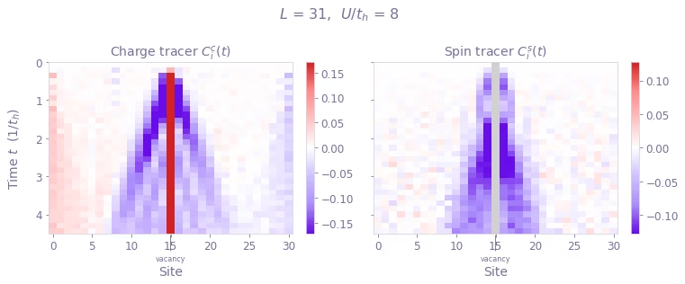
ถ้าพล็อต correlator แต่ละตัวเป็น heatmap ของปริภูมิและเวลา จะเห็น light cone ได้โดยตรง เวลาไหลลงด้านล่าง และแกนนอนคือตำแหน่งตามแนวโซ่

def plot_tracer(axis, tracer, title):
    """Draw one tracer correlator as a space-time heatmap, time flowing down."""
    # Scale from the off-centre sites. The vacancy site carries an order-one
    # change in charge density and is left to clip rather than set the scale.
    off_center = np.ones(site_count, dtype=bool)
    off_center[vacancy_site] = False
    limit = np.nanpercentile(np.abs(tracer[off_center]), 98)

    colormap = qv.QCTRL_DIVERGENT_COLORMAP.reversed().copy()
    colormap.set_bad("0.82")  # the spin tracer has no value at the vacancy

    image = axis.imshow(
        tracer.T,
        aspect="auto",
        origin="upper",
        cmap=colormap,
        vmin=-limit,
        vmax=limit,
        extent=(-0.5, site_count - 0.5, times[-1], times[0]),
        interpolation="nearest",
    )

    axis.annotate(
        "vacancy",
        xy=(vacancy_site, times[-1]),
        xytext=(vacancy_site, times[-1] + 0.55),
        ha="center",
        va="top",
        fontsize=8,
        annotation_clip=False,
        arrowprops=dict(arrowstyle="-", lw=0.8, color="0.4"),
    )

    axis.set_title(title)
    axis.set_xlabel("Site")
    return image

fig, axes = plt.subplots(1, 2, figsize=(11, 4.5), sharey=True)

charge_image = plot_tracer(
    axes[0], charge_tracer, r"Charge tracer $C^{c}_{i}(t)$"
)
spin_image = plot_tracer(axes[1], spin_tracer, r"Spin tracer $C^{s}_{i}(t)$")

axes[0].set_ylabel(r"Time $t$  $(1/t_h)$")
fig.colorbar(charge_image, ax=axes[0], fraction=0.046)
fig.colorbar(spin_image, ax=axes[1], fraction=0.046)
fig.suptitle(f"$L$ = {site_count},  $U/t_h$ = {on_site_interaction:.0f}")
fig.tight_layout()
plt.show()

ดึงความเร็วของ wavefront

แปลง heatmap เป็นตัวเลขโดยทำตามโปรโตคอลการตรวจจับจากงานวิจัยที่ตีพิมพ์ [2] ที่แต่ละช่วงเวลา ให้ทำให้โปรไฟล์เชิงพื้นที่สมมาตรรอบตำแหน่งที่ว่าง ซึ่งจะเฉลี่ยส่วนที่ไม่สมมาตรของสัญญาณรบกวนจากฮาร์ดแวร์ให้หายไป จากนั้น normalize ด้วยแอมพลิจูดนอกศูนย์กลางที่ใหญ่ที่สุด และบันทึกไซต์นอกสุดที่อยู่เหนือค่าขีดแบ่ง จากนั้นแบ่งการตรวจจับเป็นช่วงของ time step ที่ต่อเนื่องกัน และ fit เฉพาะช่วงที่ยาวที่สุด ซึ่งช่วยกันไม่ให้ transient ช่วงต้นปนเข้าไปในผลลัพธ์

def front_distance(profile, center, threshold):
    """Distance from `center` to the outermost site above a relative threshold."""
    values = np.nan_to_num(np.asarray(profile, dtype=float))
    length = values.size

    symmetrized = values.copy()
    for site in range(length):
        mirror = 2 * center - site
        if 0 <= mirror < length:
            symmetrized[site] = 0.5 * (values[site] + values[mirror])

    amplitude = np.abs(symmetrized)
    off_center = np.ones(length, dtype=bool)
    off_center[center] = False

    peak = amplitude[off_center].max()
    if peak <= 0.0:
        return np.nan
    above = np.flatnonzero((amplitude / peak > threshold) & off_center)
    return float(np.abs(above - center).max()) if above.size else np.nan

def longest_run(mask):
    """Indices of the longest run of consecutive True values."""
    best, current = [], []
    for index, keep in enumerate(mask):
        current = current + [index] if keep else []
        if len(current) > len(best):
            best = current
    return np.array(best, dtype=int)

def front_velocity(tracer, center, threshold=0.3, quantile=0.75, min_block=5):
    """Fit front position against time, using only the longest contiguous run."""
    distances = np.array(
        [
            front_distance(tracer[:, k], center, threshold)
            for k in range(tracer.shape[1])
        ]
    )
    edge = max(center, tracer.shape[0] - 1 - center)
    usable = (
        np.isfinite(distances) & (distances >= 2) & (distances <= edge - 2)
    )

    block = longest_run(usable)
    if block.size < min_block:
        return np.nan, distances, np.array([], dtype=int), np.nan

    candidates = [
        stats.theilslopes(distances[block[:k]], times[block[:k]]).slope
        for k in range(min_block, block.size + 1)
    ]
    cutoff = np.quantile(candidates, quantile)
    keep = max(i for i, value in enumerate(candidates) if value >= cutoff)

    fit_block = block[: keep + min_block]
    slope, intercept = np.polyfit(times[fit_block], distances[fit_block], 1)
    return float(slope), distances, fit_block, float(intercept)

ความเร็วที่ fit ได้ขึ้นกับค่าขีดแบ่งในการตรวจจับและ quantile ที่ใช้ตัดทอน และความไวนี้มีผลมากกว่า shot noise ให้สแกนทั้งสองค่าแล้วรายงานค่ามัธยฐานพร้อมช่วงครอบคลุมทั้งหมด เหมือนที่การวิเคราะห์ในงานวิจัยทำ

thresholds = [0.15, 0.225, 0.30, 0.375, 0.45]
quantiles = [0.60, 0.675, 0.75, 0.825, 0.90]

def velocity_envelope(tracer, center):
    """Median, minimum, and maximum velocity over the parameter scan."""
    values = [
        front_velocity(tracer, center, threshold=p, quantile=q)[0]
        for p in thresholds
        for q in quantiles
    ]
    values = np.array([v for v in values if np.isfinite(v)])
    if values.size == 0:
        return np.nan, np.nan, np.nan
    return float(np.median(values)), float(values.min()), float(values.max())

charge_velocity, charge_low, charge_high = velocity_envelope(
    charge_tracer, vacancy_site
)
spin_velocity, spin_low, spin_high = velocity_envelope(
    spin_tracer, vacancy_site
)

_, charge_front, charge_block, charge_intercept = front_velocity(
    charge_tracer, vacancy_site
)
_, spin_front, spin_block, spin_intercept = front_velocity(
    spin_tracer, vacancy_site
)

print(f"v_c = {charge_velocity:.2f}  [{charge_low:.2f}, {charge_high:.2f}]")
print(f"v_s = {spin_velocity:.2f}  [{spin_low:.2f}, {spin_high:.2f}]")
print(f"v_s / v_c = {spin_velocity / charge_velocity:.2f}")

v_c = 1.93  [1.81, 2.18]
v_s = 1.61  [1.23, 2.12]
v_s / v_c = 0.83

PUBLISHED = {"charge": 1.78, "spin": 1.46}

edge = max(vacancy_site, site_count - 1 - vacancy_site)
fig, axis = plt.subplots(figsize=(7, 4.6))

axis.axhspan(0, 2, color="0.92", zorder=0)
axis.axhspan(edge - 2, edge + 2, color="0.92", zorder=0)

series = [
    (
        "charge",
        "$v_c$",
        charge_front,
        charge_block,
        charge_velocity,
        charge_intercept,
        charge_low,
        charge_high,
        "C0",
        "o",
    ),
    (
        "spin",
        "$v_s$",
        spin_front,
        spin_block,
        spin_velocity,
        spin_intercept,
        spin_low,
        spin_high,
        "C1",
        "s",
    ),
]

for name, sym, front, block, v, b, lo, hi, color, marker in series:
    excluded = np.setdiff1d(np.arange(front.size), block)
    axis.plot(
        times[excluded],
        front[excluded],
        marker,
        color=color,
        markersize=5,
        markerfacecolor="none",
        alpha=0.45,
        zorder=2,
    )
    axis.plot(
        times[block],
        front[block],
        marker,
        color=color,
        markersize=5,
        label=f"{name}, {sym} = {v:.2f} [{lo:.2f}, {hi:.2f}]",
        zorder=3,
    )

    span = times[block]
    anchor = v * span[0] + b
    axis.plot(
        span,
        v * (span - span[0]) + anchor,
        "-",
        color=color,
        lw=1.6,
        zorder=4,
    )
    axis.fill_between(
        span,
        lo * (span - span[0]) + anchor,
        hi * (span - span[0]) + anchor,
        color=color,
        alpha=0.15,
        zorder=1,
    )
    axis.plot(
        span,
        PUBLISHED[name] * (span - span[0]) + anchor,
        "--",
        color=color,
        lw=1.2,
        alpha=0.8,
        zorder=4,
    )

axis.plot([], [], "--", color="0.4", lw=1.2, label="published [2]")
axis.plot(
    [],
    [],
    "o",
    color="0.5",
    markerfacecolor="none",
    label="excluded from fit",
)

axis.set_xlabel(r"Time $t$  $(1/t_h)$")
axis.set_ylabel("Front distance from vacancy (sites)")
axis.set_xlim(0, times[-1])
axis.set_ylim(
    0, min(edge + 1, np.nanmax(np.r_[charge_front, spin_front]) + 3)
)
axis.legend(loc="upper left", frameon=False, fontsize=9)
axis.set_title(
    f"L = {site_count}, $U/t_h$ = {on_site_interaction:.0f}, front propagation",
    fontsize=11,
)

fig.tight_layout()
plt.show()

การวาดจุดที่ตรวจจับได้กลับลงบน heatmap ช่วยให้เห็นว่าอัลกอริทึมตามขอบนำหน้าได้หรือไม่ เครื่องหมายทึบคือจุดที่ตรวจจับได้และถูกนำไป fit ส่วนเครื่องหมายโปร่งคือจุดที่ถูกตัดออกด้วยกฎการมาสก์ เพราะอยู่ใกล้ ตำแหน่งที่ว่างเกินไป ใกล้ปลายโซ่เกินไป หรือช้าเกินไปจนแนวหน้า ขยายกว้างและตำแหน่งไม่คมชัดอีกแล้ว เส้นประคือเส้น fit บน ช่วงเวลาที่ใช้ และความชันของมันคือความเร็วที่แสดงในชื่อของแต่ละแผง

คอลัมน์ของตำแหน่งที่ว่างถูกทำเครื่องหมายไว้ใต้แกน ค่า charge ถูกตัดที่ตรงนั้นเพราะค่าของมัน อยู่ในระดับหนึ่ง ส่วน spin ไม่มีค่าที่ตรงนั้น จึงวาดเป็นสีเทา

กรวย charge เปิดกว้างกว่ากรวย spin การรบกวนทั้งสองชนิดทิ้งตำหนิเดียวกัน ในจังหวะเดียวกัน และแผ่ออกไปด้วยความเร็วต่างกัน

def plot_tracer_front(axis, tracer, front, block, velocity, intercept, title):
    """Overlay the detected wavefront and the fitted cone on a tracer heatmap."""
    image = plot_tracer(axis, tracer, title)

    excluded = np.setdiff1d(np.arange(front.size), block)
    for index, filled in ((block, True), (excluded, False)):
        good = index[np.isfinite(front[index])]
        if good.size == 0:
            continue
        for sign in (-1, 1):
            axis.plot(
                vacancy_site + sign * front[good],
                times[good],
                "o",
                markersize=4,
                color="k",
                markerfacecolor="k" if filled else "none",
                markeredgewidth=0.9,
                alpha=1.0 if filled else 0.4,
            )

    span = times[block]
    for sign in (-1, 1):
        axis.plot(
            vacancy_site + sign * (velocity * span + intercept),
            span,
            "--",
            color="k",
            lw=1.5,
        )

    axis.set_title(f"{title}    $v$ = {velocity:.2f}")
    return image

fig, axes = plt.subplots(1, 2, figsize=(11, 4.5), sharey=True)

charge_image = plot_tracer_front(
    axes[0],
    charge_tracer,
    charge_front,
    charge_block,
    charge_velocity,
    charge_intercept,
    r"Charge tracer $C^{c}_{i}(t)$",
)
spin_image = plot_tracer_front(
    axes[1],
    spin_tracer,
    spin_front,
    spin_block,
    spin_velocity,
    spin_intercept,
    r"Spin tracer $C^{s}_{i}(t)$",
)

axes[0].set_ylabel(r"Time $t$  $(1/t_h)$")
fig.colorbar(charge_image, ax=axes[0], fraction=0.046)
fig.colorbar(spin_image, ax=axes[1], fraction=0.046)
fig.suptitle(f"$L$ = {site_count},  $U/t_h$ = {on_site_interaction:.0f}")
fig.tight_layout()
plt.show()

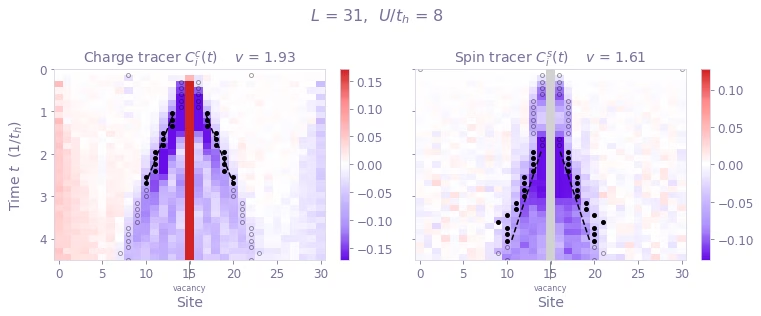
แนวหน้า charge วิ่งเร็วกว่าแนวหน้า spin โฮลในพื้นหลัง Mott หนึ่งมิติไม่ได้เคลื่อนที่เหมือนอิเล็กตรอน แต่จะแตกเป็น holon ที่พา charge กับ spinon ที่พาการรบกวนของ spin และที่ $U/t_h = 8$ spinon เป็นตัวที่ช้ากว่า

ลำดับนี้ขึ้นกับอันตรกิริยา ที่ $U = 0$ โมเดลเป็นเฟอร์มิออนอิสระที่มี $v_c = 2$ และ $v_s = 4$ ดังนั้น spin เร็วกว่า แรงผลักทำให้การขนส่ง spin ถูกกดลงโดยแทบไม่แตะการขนส่ง charge และเมื่อถึง $U/t_h = 8$ ค่าจากฮาร์ดแวร์ที่ตีพิมพ์คือ $v_c = 1.78$ และ $v_s = 1.46$ [2] การรันซ้ำด้วยค่า $U$ หลายค่าแล้วพล็อต $v_s / v_c$ จะแสดงจุดตัดผ่านของลำดับนี้

ข้อควรระวังเกี่ยวกับตัวเลข การตรวจจับด้วยค่าขีดแบ่งมีความเอนเอียงต่ำลงเล็กน้อย จึงคาดได้ว่าความเร็ว charge จะต่ำกว่าค่าที่ตีพิมพ์ไม่กี่เปอร์เซ็นต์ ช่วงครอบคลุมของ spin กว้างเพราะ connected correlator อยู่ใกล้ noise floor มากกว่า นี่คือเหตุผลที่รายงานค่ามัธยฐานของการสแกนแทนการ fit ครั้งเดียว

เอกสารอ้างอิง

[1] Essler, F. H. L., Frahm, H., Gohmann, F., Klumper, A., & Korepin, V. E. (2005). The One-Dimensional Hubbard Model. Cambridge University Press.

[2] Hartnett, G. S., Najafi, K. S., Khindanov, A., Liao, H., Schutzman, M., Hush, M. R., Biercuk, M. J., & Baum, Y. (2026). Fast, accurate, high-resolution simulation of large-scale Fermi-Hubbard models on a digital quantum processor. arXiv:2605.04025.