การจำลอง kicked Ising model ด้วยฟังก์ชัน TEM

วิธี Tensor-network Error Mitigation (TEM) ของ Algorithmiq เป็นอัลกอริทึมแบบผสมผสานระหว่างควอนตัมและคลาสสิก ที่ออกแบบมาเพื่อทำการลดข้อผิดพลาดจากสัญญาณรบกวนทั้งหมดในขั้นตอนการประมวลผลหลังการทดลองแบบคลาสสิก ด้วย TEM ผู้ใช้สามารถคำนวณค่าคาดหวังของ observable โดยลดข้อผิดพลาดที่เกิดจากสัญญาณรบกวนที่หลีกเลี่ยงไม่ได้บนฮาร์ดแวร์ควอนตัม ด้วยความแม่นยำและประสิทธิภาพด้านต้นทุนที่เพิ่มขึ้น ทำให้เป็นตัวเลือกที่น่าสนใจอย่างมากสำหรับนักวิจัยควอนตัมและผู้ประกอบวิชาชีพในอุตสาหกรรม

บทช่วยสอนนี้แสดงให้เห็นว่า TEM สามารถได้รับผลลัพธ์ที่มีความหมายสำหรับพลศาสตร์ของระบบควอนตัม ซึ่งจะไม่สามารถเข้าถึงได้หากไม่มีการลดข้อผิดพลาด และต้องการทรัพยากรควอนตัมมากกว่าอย่างมีนัยสำคัญหากใช้วิธีลดข้อผิดพลาดอื่น เช่น PEC และ ZNE

การประมาณการใช้งาน: โน้ตบุ๊กนี้ใช้ประมาณ 10 QPU นาทีบนอุปกรณ์ Heron r3 เวลาการรันอาจแตกต่างกันอย่างมีนัยสำคัญขึ้นอยู่กับอุปกรณ์ที่เลือก ค่าประมาณการใช้งานต่อส่วนสามารถดูได้ด้านล่าง

รันการทดลองฟิสิกส์หลายอนุภาคที่มีการลดข้อผิดพลาดด้วยฟังก์ชัน TEM

บทช่วยสอนนี้อ้างอิงจาก: L. E. Fischer et al., Nat. Phys. (2026) ซึ่งกล่าวถึงการจำลองจริงบนฮาร์ดแวร์ควอนตัมที่มีขนาดถึง 91 qubit ในบทช่วยสอนนี้เราจะสร้างการจำลองที่คล้ายกันในขนาดวงจรที่เล็กกว่า

โมเดล kicked Ising สอดคล้องกับโมเดล Ising ปกติ:

$\hat{H}_{\text{I}} = J \sum_{n=0}^{N-2} \hat{Z}_n \hat{Z}_{n+1} + h \sum_{n=0}^{N-1} \hat{Z}_n$

ซึ่งมีการใช้ transverse kick:

$\hat{H}_{K} = b \sum_{n=0}^{N-1} \hat{X}_n$

เป้าหมายคือการจำลองพลศาสตร์ของสถานะภายใต้ Hamiltonian ของ transverse kicked Ising ซึ่งการวิวัฒนาการตามเวลาสามารถนำไปใช้งานได้โดย Floquet unitary $\hat{U}_{\text{KI}} = e^{-i \hat{H}_K} e^{-i \hat{H}_I}$ สถานะเริ่มต้นที่จะวิวัฒนาการคือสถานะที่ qubit แรกอยู่ในสถานะ $|+\rangle$ ในขณะที่สถานะอื่นๆ จับคู่กันและตั้งค่าใน Bell state $(|00\rangle + |11\rangle)/\sqrt{2}$

ปริมาณที่เราต้องการสังเกตคือฟังก์ชันสหสัมพันธ์ บทความอ้างอิง อธิบายว่าปริมาณนี้สามารถเขียนใหม่เป็น $\hat{X}$ Pauli operator บน $n^{th}$ qubit ได้ หลังจากจำนวนขั้นเวลาทางฟิสิกส์ $t$ เราคำนวณค่าของ Pauli operator $\hat{X}_{n=t}$ ขึ้นอยู่กับพารามิเตอร์ของระบบ ค่าของ observable นี้เท่ากับค่าที่สามารถคำนวณได้อย่างแม่นยำ หรือจำลองได้โดยวิธีการโดยประมาณเท่านั้น โดยเฉพาะสำหรับ $|J|=|b|=\pi/4$ จะเท่ากับ $[\cos(2h)]^t$ ซึ่งเป็นค่าที่เราจะใช้เป็นเกณฑ์มาตรฐานสำหรับผลลัพธ์ของบทช่วยสอนนี้ นอกจากนี้ ณ ขั้นเวลาที่กำหนด $t$ ค่า $\langle\hat{X}_{n\neq t}\rangle$ เป็นศูนย์ สำหรับรายละเอียดในการรับค่าเหล่านี้ และสำหรับการเปรียบเทียบกับผลลัพธ์การจำลองแบบคลาสสิกโดยประมาณนอกเหนือจากพารามิเตอร์เหล่านี้ โปรดดู L. E. Fischer et al., Nat. Phys. (2026)

TEM ทำงานโดยการระบุสัญญาณรบกวนสำหรับแต่ละเลเยอร์ที่ไม่ซ้ำกันของ two-qubit gate ในวงจรก่อน รวมถึงการระบุข้อผิดพลาดในการอ่านค่า จากนั้นวงจรจะถูกดำเนินการบนเครื่องควอนตัม สุดท้ายการลดข้อผิดพลาดด้วย tensor network จะถูกดำเนินการบนทรัพยากรแบบคลาสสิกใน IBM Cloud® และค่าที่ถูกลดข้อผิดพลาดจะถูกส่งคืน ในตัวอย่างนี้วงจรมีสองเลเยอร์ที่ไม่ซ้ำกันที่ต้องระบุ

การตั้งค่า

เป็นข้อกำหนดเบื้องต้น ให้ตรวจสอบว่าได้ติดตั้ง dependencies ที่จำเป็นแล้ว

%pip install numpy matplotlib qiskit qiskit-ibm-catalog qiskit-ibm-runtime pylatexenc qiskit_qasm3_import

import os
from matplotlib import pyplot as plt
import numpy as np

from qiskit.quantum_info import SparsePauliOp
from qiskit.qasm3 import load

from qiskit_ibm_catalog import QiskitFunctionsCatalog

การลดข้อผิดพลาดด้วย TEM

เราจัดเตรียมวงจรที่นำ kicked Ising model มาใช้งานตามที่อธิบายไว้ด้านบน วงจรถูกเตรียมดังนี้ ขั้นแรกมีช่วงการเตรียมสถานะ ซึ่ง qubit แรกอยู่ในสถานะ $|+\rangle$ ในขณะที่สถานะอื่นๆ อยู่ใน Bell pairs $(|00\rangle + |11\rangle)/\sqrt{2}$ ตามด้วยโครงสร้าง brickwork ที่นำการวิวัฒนาการ unitary $\hat{U}_{\text{KI}}$ มาใช้ จำนวนขั้นเวลาทางฟิสิกส์สอดคล้องกับ $t/2$ เลเยอร์ของวงจร โค้ดต่อไปนี้ดาวน์โหลดไฟล์ QASM สองไฟล์ที่จำเป็นสำหรับบทช่วยสอนนี้

# Download required QASM files
import urllib

urllib.request.urlretrieve(
    "https://ibm.box.com/shared/static/swy5jtq309b0xpzluzlmsmj908yphes8.qasm",
    "ki_30q.qasm",
)
urllib.request.urlretrieve(
    "https://ibm.box.com/shared/static/et3gkodonw6gsp2trs43lzaozrdtiu7s.qasm",
    "ki_12q.qasm",
)

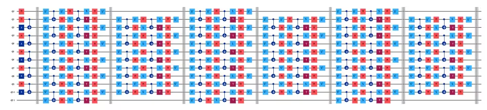
เราสามารถแสดงภาพวงจรขนาดเล็กที่มี 12 qubit และหกขั้นเวลา:

# Parameters of the kicked Ising model
h = 0.0
num_qubits = 12
t_steps = 6

# Load the circuit for the kicked Ising model
small_circuit = load("ki_12q.qasm")

# Draw the circuit
small_circuit.draw("mpl", scale=0.25, fold=-1)

ถัดไป สร้าง observable $\hat{X}_{n=t}$ โดยสร้างเป็น Pauli string ง่ายๆ ที่มีลำดับตรงกับที่ Qiskit ใช้:

def xt_observable(n_qubits, t_steps):
    pauli_str = "".join(["I" * t_steps, "X", "I" * (n_qubits - t_steps - 1)])
    pauli_str = pauli_str[::-1]  # Reverse the string to match qiskit order
    return SparsePauliOp(data=pauli_str, coeffs=1.0)

ในตัวอย่างขนาดเล็กที่มี 12 qubit observable มีลักษณะดังนี้:

# Build the observable for the kicked Ising model
small_observable = xt_observable(n_qubits=12, t_steps=6)
print(small_observable)

SparsePauliOp(['IIIIIXIIIIII'],
              coeffs=[1.+0.j])

Qiskit Functions ใช้ PUB เป็นวิธีรวบรวม input ในกรณีของเรา ให้พิจารณาวงจรและ observable เดี่ยวเป็น PUB:

# Collect the input PUBs, in this case composed of a
# single circuit and observable
pubs = [(small_circuit, [small_observable])]

ถัดไป เราเข้าถึงฟังก์ชัน TEM ก่อนอื่น ตั้งค่าการตรวจสอบสิทธิ์ที่จำเป็นสำหรับ IBM Cloud และเลือก backend จากอุปกรณ์ที่มีอยู่ token, backend ที่มีอยู่ และชื่อทรัพยากรคลาวด์ (CRN) ที่สอดคล้องกันสามารถรับได้โดยการเข้าสู่ระบบบัญชีของคุณบน IBM Quantum Platform dashboard

# Set IBM Quantum credentials and backend configuration
personal_token = os.environ.get(
    "QISKIT_IBM_TOKEN", "<API-KEY>"
)  # Replace with your personal token or set the environment variable
channel = "ibm_quantum_platform"
crn = "your_crn"  # Replace with the Cloud Resource Name (CRN)

# Select the QPU backend
backend_name = "ibm_qpu_name"  # Replace with your desired backend's name

โหลดฟังก์ชัน TEM จาก Qiskit Functions Catalog:

# Load the TEM function from the Qiskit Functions Catalog
catalog = QiskitFunctionsCatalog(
    channel=channel,
    token=personal_token,
    instance=crn,
)
tem = catalog.load("algorithmiq/tem")

ตอนนี้เราสามารถรันการทดลองบนวงจร kicked Ising ด้วยการลดข้อผิดพลาดที่ TEM จัดเตรียมไว้ การใช้การตั้งค่าเริ่มต้น TEM สามารถรันได้ง่ายๆ โดยมีเวลาการรัน QPU ที่คาดหวังประมาณ 2.5 นาที ขึ้นอยู่กับ QPU:

tem_job = tem.run(pubs=pubs, backend_name=backend_name)

ด้วยตัวเลือกเริ่มต้น ฟังก์ชัน TEM จะรันงานสามชิ้นบนคอมพิวเตอร์ควอนตัม: การเรียนรู้สัญญาณรบกวน การลดข้อผิดพลาดในการอ่านค่า และการสุ่มตัวอย่างวงจร จำนวน shots ที่แต่ละงานใช้สามารถเปลี่ยนแปลงได้ในตัวเลือกที่ส่งไปยังฟังก์ชัน โดยค่าเริ่มต้น พารามิเตอร์เหล่านี้ถูกตั้งค่าให้บรรลุความแม่นยำ 0.05 ในค่าคาดหวังที่ถูกลดข้อผิดพลาด คุณสามารถตรวจสอบสถานะของงานบน IBM Quantum Platform dashboard หรือด้วย:

print(tem_job.status())

QUEUED

เมื่อสถานะเป็น DONE เราสามารถตรวจสอบผลลัพธ์ดิบและที่ถูกลดข้อผิดพลาด tem_evs ที่กำหนดด้านล่างคือค่าคาดหวังของ observable ที่ร้องขอ ในกรณีนี้คือ observable เดียว $\langle \hat X_{n=t}\rangle$ และ tem_std คือส่วนเบี่ยงเบนมาตรฐานที่สอดคล้องกัน

# Get the results of the TEM job
tem_results = tem_job.result()[
    0
]  # Get the first and only result from the job
tem_evs = tem_results.data.evs[0]
tem_std = tem_results.data.stds[0]

print(f"TEM Result: {tem_evs:.3f} ± {tem_std:.3f}")

TEM Result: 1.031 ± 0.046

เราสามารถตรวจสอบว่าใช้เวลาการรันควอนตัมเท่าใดสำหรับแต่ละการเรียกที่ IBM Quantum Platform หรือโดยการตรวจสอบ metadata ของผลลัพธ์จากโค้ด Python

# Get the TEM job runtime
tem_runtime = tem_job.result().metadata["resource_usage"][
    "RUNNING: EXECUTING_QPU"
]["QPU_TIME"]

print(f"TEM Runtime: {tem_runtime} seconds")

TEM Runtime: 155.0 seconds

ปรับแต่งพารามิเตอร์ TEM และตัวเลือกขั้นสูง

ฟังก์ชัน TEM มีตัวเลือกขั้นสูงหลายอย่างเพื่อปรับแต่งเวิร์กโฟลว์การลดข้อผิดพลาดของคุณ ตัวเลือกเหล่านี้ช่วยให้คุณควบคุมความแม่นยำ จำนวน shots กลยุทธ์การเรียนรู้สัญญาณรบกวน และพารามิเตอร์อื่นๆ เพื่อให้เหมาะสมกับข้อกำหนดของการทดลองและทรัพยากรควอนตัมที่มีอยู่มากขึ้น

ตัวเลือกขั้นสูงที่ใช้บ่อยได้แก่:

• precision: ระบุความแม่นยำเป้าหมายสำหรับค่าคาดหวังที่ถูกลดข้อผิดพลาด
• default_shots: แทนที่จะใช้ precision คุณสามารถระบุจำนวน shots ที่ใช้โดยงานการวัด
• tem_max_bond_dimension: มิติพันธะสูงสุดที่ใช้ใน tensor network
• tem_compression_cutoff: ค่าตัดทอนที่จะใช้สำหรับ tensor network
• ตัวเลือกการเรียนรู้สัญญาณรบกวน: กำหนดค่าว่าจะระบุสัญญาณรบกวนอย่างไร เช่น จำนวนการทำซ้ำหรือวงจรการปรับเทียบเฉพาะ
• private: ให้วงจรและผลการทดลองเป็นส่วนตัวสำหรับคุณ และปิดใช้งานการดาวน์โหลดผลลัพธ์งานหลายครั้ง

ดูรายการตัวเลือกที่รองรับทั้งหมดและคำอธิบายได้ที่ เอกสาร TEM หรือ Qiskit Functions Catalog คุณสามารถปรับพารามิเตอร์เหล่านี้เพื่อสร้างความสมดุลระหว่างเวลาการรัน การใช้ทรัพยากร และความแม่นยำของผลลัพธ์ คุณสามารถส่งตัวเลือกเหล่านี้เป็น dictionary ไปยังอาร์กิวเมนต์ options เมื่อรันฟังก์ชัน TEM:

options = {
    "default_shots": 10_000,
    "tem_max_bond_dimension": 512,
    "tem_compression_cutoff": 1e-16,
    # This option helps optimizing the measurement
    # stage since the observable is strongly biased
    # toward the X operator for all the qubits.
    "compute_shadows_bias_from_observable": True,
    # set to True to keep experiment results private,
    # recommended for confidential circuits
    "private": False,
}

ตัวเลือกแบบกำหนดเองสำหรับตัวเรียนรู้สัญญาณรบกวนก็สามารถส่งได้เช่นกัน ซึ่งเป็นไปตามคำนิยามที่ใช้ใน Qiskit Runtime NoiseLearnerOptions:

nl_options = {
    "num_randomizations": 32,
    "max_layers_to_learn": 2,
    "shots_per_randomization": 128,
    "layer_pair_depths": [0, 1, 2, 4, 16, 32],
}

# add noise learning options to the overall options
options |= nl_options

รันการทดลองซ้ำด้วยตัวเลือกแบบกำหนดเองเหล่านี้ที่ปรับแต่งสำหรับวงจรของเรา เวลาการรันที่คาดหวังอยู่ที่ประมาณสี่ QPU นาที

tem_job_custom = tem.run(
    pubs=pubs, backend_name=backend_name, options=options
)

หากงานไม่ได้ตั้งค่าเป็นส่วนตัว เราสามารถกู้คืนผลลัพธ์ในภายหลังได้ โดยบันทึก job ID ที่แสดงที่นี่และใช้ tem_job_custom = catalog.get_job_by_id("your-job-id")

job_id = tem_job_custom.job_id
print(f"Job ID: {job_id}")

Job ID: 1ba10094-a541-457a-9287-dbd49306d12d

results_custom = tem_job_custom.result()
tem_evs = results_custom[0].data.evs[0]
tem_std = results_custom[0].data.stds[0]

print(f"TEM Result: {tem_evs:.3f} ± {tem_std:.3f}")

TEM Result: 0.956 ± 0.018

ตอนนี้เราสามารถตรวจสอบผลลัพธ์และ metadata เพื่อรับข้อมูลเชิงลึกเกี่ยวกับการทดลอง:

metadata_custom = results_custom[0].metadata

unmitigated_evs = metadata_custom["evs_non_mitigated"][0]
unmitigated_stds = metadata_custom["stds_non_mitigated"][0]
print(f"Unmitigated Result: {unmitigated_evs:.3f} ± {unmitigated_stds:.3f}")

# Exact result for the kicked Ising model from the reference paper
exact_evs = np.cos(2 * h) ** t_steps
print("Exact Result:", exact_evs)

Unmitigated Result: 0.894 ± 0.015
Exact Result: 1.0

# Plot comparing the different expectation values
plt.bar(
    ["Unmitigated", "TEM"],
    [unmitigated_evs, tem_evs],
    yerr=[unmitigated_stds, tem_std],
    color=["grey", "c"],
)
plt.hlines(y=exact_evs, xmin=-0.5, xmax=1.5, colors="r", linestyles="dashed")
plt.ylabel("Expectation Value")
plt.ylim(0, 1.1)
plt.show()

สุดท้าย เราสามารถตรวจสอบผลกระทบของตัวเลือกแบบกำหนดเองต่อ QPU และเวลาการรันแบบคลาสสิก:

# Get the metadata of the TEM job
job_metadata = results_custom.metadata

# Get the runtime of the TEM job
qpu_runtime = job_metadata["resource_usage"]["RUNNING: EXECUTING_QPU"][
    "QPU_TIME"
]
classical_runtime = (
    job_metadata["resource_usage"]["RUNNING: OPTIMIZING_FOR_HARDWARE"][
        "CPU_TIME"
    ]
    + job_metadata["resource_usage"]["RUNNING: POST_PROCESSING"]["CPU_TIME"]
)

print(f"QPU Runtime: {qpu_runtime} seconds")
print(f"Classical Runtime: {classical_runtime} seconds")

QPU Runtime: 342.0 seconds
Classical Runtime: 107.632604 seconds

ขยาย TEM ไปสู่วงจรขนาดใหญ่

วงจรขนาดใหญ่สามารถรันด้วยฟังก์ชัน TEM ได้ในหลักการ อย่างไรก็ตาม สิ่งสำคัญคือต้องตระหนักถึงข้อจำกัดของทรัพยากรแบบคลาสสิก เนื่องจาก TEM ทำงานบน IBM Cloud runners ซึ่งอาจมีเวลาการรันที่นานมาก สำหรับวงจรขนาดใหญ่มาก ติดต่อทีมสนับสนุน TEM ที่ qiskit_ibm@algorithmiq.fi

ที่นี่เราจะรันตัวอย่างด้วยวงจร 30 qubit ขนาดใหญ่ระดับยูทิลิตี้ โดยปรับพารามิเตอร์ TEM เพื่อความเร็วมากกว่าความแม่นยำ

# Kicked Ising model parameters
n_qubits = 30
t_steps = 15
h = 0.0

# Load the circuit for the kicked Ising model
circuit = load("ki_30q.qasm")

# Build the observable for the kicked Ising model
observable = xt_observable(n_qubits=n_qubits, t_steps=t_steps)

# Collect the input PUBs, in this case composed of a
# single circuit and observable
pubs = [(circuit, [observable])]

กำหนดตัวเลือกที่เน้นประสิทธิภาพ:

options = {
    "num_randomizations": 32,
    "max_layers_to_learn": 2,
    "shots_per_randomization": 128,
    "layer_pair_depths": [0, 1, 2, 4, 16, 32, 64],
    "default_shots": 5_000,
    "tem_max_bond_dimension": 128,
    "tem_compression_cutoff": 1e-10,
    "compute_shadows_bias_from_observable": True,
    "private": False,
}

สุดท้าย รันการทดลอง รับผลลัพธ์ และแสดงผล ซึ่งจะใช้เวลาประมาณ 3.5 QPU นาที

tem_job_large = tem.run(pubs=pubs, backend_name=backend_name, options=options)

job_id = tem_job_large.job_id
print(f"Job ID: {job_id}")

Job ID: 9f3f190f-f4b0-4dcb-bb83-5f71f37d0d77

results_large = tem_job_large.result()
tem_evs = results_large[0].data.evs[0]
tem_std = results_large[0].data.stds[0]

print(f"TEM Result: {tem_evs:.3f} ± {tem_std:.3f}")

# Get the metadata of the TEM job
job_metadata = tem_job_large.result().metadata

# Get the runtime of the TEM job
qpu_runtime = job_metadata["resource_usage"]["RUNNING: EXECUTING_QPU"][
    "QPU_TIME"
]
classical_runtime = (
    job_metadata["resource_usage"]["RUNNING: OPTIMIZING_FOR_HARDWARE"][
        "CPU_TIME"
    ]
    + job_metadata["resource_usage"]["RUNNING: POST_PROCESSING"]["CPU_TIME"]
)

print(f"QPU Runtime: {qpu_runtime} seconds")
print(f"Classical Runtime: {classical_runtime} seconds")

TEM Result: 0.794 ± 0.026
QPU Runtime: 203.0 seconds
Classical Runtime: 251.71805499999996 seconds

# Plot comparing the different expectation values
metadata_large = results_large[0].metadata
unmitigated_evs = metadata_large["evs_non_mitigated"][0]
unmitigated_stds = metadata_large["stds_non_mitigated"][0]

exact_evs = np.cos(2 * h) ** t_steps

plt.bar(
    ["Unmitigated", "TEM"],
    [unmitigated_evs, tem_evs],
    yerr=[unmitigated_stds, tem_std],
    color=["grey", "c"],
)
plt.hlines(y=exact_evs, xmin=-0.5, xmax=1.5, colors="r", linestyles="dashed")
plt.ylabel("Expectation Value")
plt.ylim(0, 1.1)
plt.show()