แนะนำ Qiskit AI-powered transpiler

เวลาใช้งานโดยประมาณ: 5 นาที บน IBM Heron (หมายเหตุ: นี่เป็นการประมาณการเท่านั้น เวลาในการรันจริงอาจแตกต่างกัน)

ผลลัพธ์การเรียนรู้

หลังจากผ่าน tutorial นี้ ผู้ใช้ควรเข้าใจ:

• วิธีใช้ AI-powered transpiler (generate_ai_pass_manager) เป็นทางเลือกทดแทน Transpiler มาตรฐาน
• วิธีที่ AI-powered transpiler เปรียบเทียบกับ Transpiler ค่าเริ่มต้นในแง่ของ two-qubit depth จำนวน Gate และเวลา transpilation
• วิธีใช้ mirror circuits เพื่อประเมินคุณภาพการ transpilation ผ่านการรันบนฮาร์ดแวร์จริง

ข้อกำหนดเบื้องต้น

เราแนะนำให้ผู้ใช้มีความคุ้นเคยกับหัวข้อต่อไปนี้ก่อนผ่าน tutorial นี้:

• Transpile circuits
• Configure preset pass managers
• AI-powered transpiler passes

พื้นหลัง

Qiskit AI-powered transpiler แนะนำ transpilation passes ที่ใช้ machine learning ซึ่งสามารถผลิต Circuit ที่สั้นกว่าและมีประสิทธิภาพด้านฮาร์ดแวร์มากกว่าวิธี heuristic แบบดั้งเดิมอย่าง SABRE Circuit ที่สั้นกว่าสะสม noise น้อยกว่า ซึ่งปรับปรุงคุณภาพผลลัพธ์บนฮาร์ดแวร์ quantum จริงโดยตรง

ใน tutorial นี้เราเปรียบเทียบกลยุทธ์การ transpilation สองอย่าง:

กลยุทธ์	API
ค่าเริ่มต้น	generate_preset_pass_manager(optimization_level=3, ...)
AI	generate_ai_pass_manager(optimization_level=1, ai_optimization_level=3, ...)

เราวัดสาม metrics สำหรับแต่ละกลยุทธ์: two-qubit gate depth, จำนวน gate รวม และ เวลา transpilation

การ benchmark ของ AI-powered transpiler

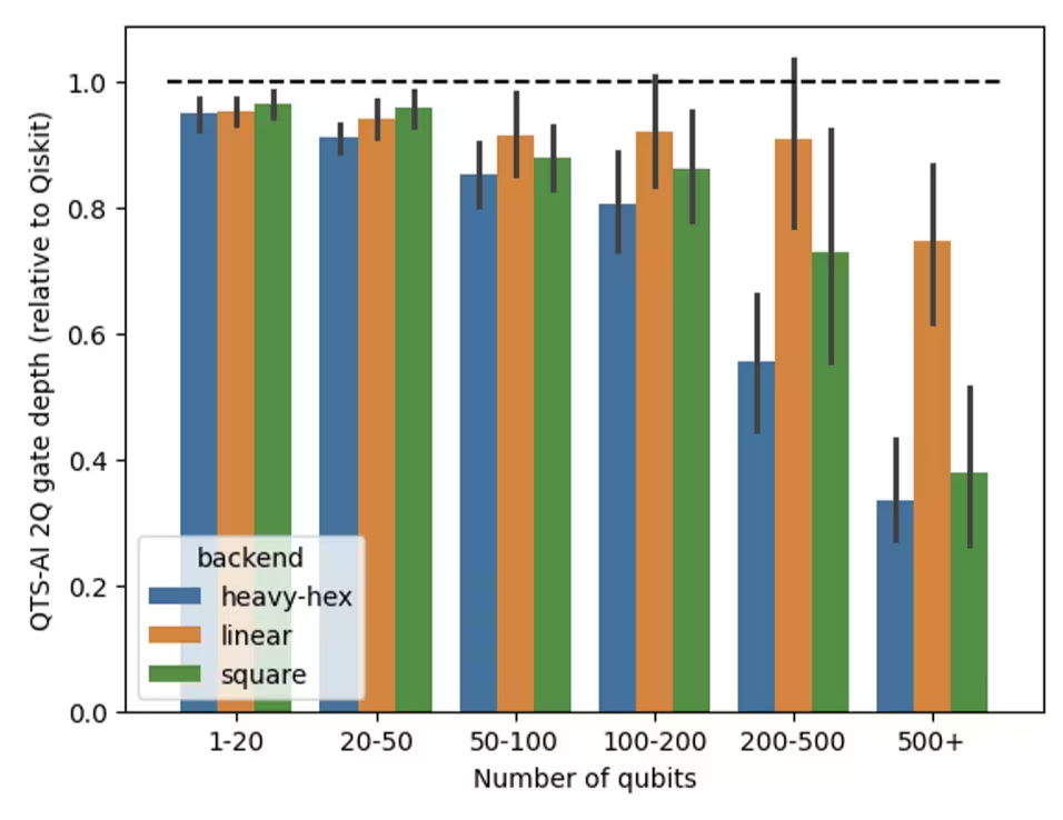
ในการทดสอบ benchmarking AI-powered transpiler สร้าง Circuit ที่ตื้นกว่าและมีคุณภาพสูงกว่าเมื่อเทียบกับ Qiskit transpiler มาตรฐานอย่างสม่ำเสมอ สำหรับการทดสอบเหล่านี้ เราใช้กลยุทธ์ pass manager ค่าเริ่มต้นของ Qiskit ซึ่งกำหนดค่าด้วย generate_preset_pass_manager แม้ว่ากลยุทธ์ค่าเริ่มต้นนี้มักมีประสิทธิภาพดี แต่อาจประสบปัญหากับ Circuit ที่ใหญ่หรือซับซ้อนกว่า ในทางตรงกันข้าม AI-powered passes ทำให้จำนวน two-qubit gate ลดลงเฉลี่ย 24% และความลึกของ Circuit ลดลง 36% สำหรับ Circuit ขนาดใหญ่ (100+ qubits) เมื่อ transpile ไปยัง heavy-hex topology ของ IBM Quantum® hardware สำหรับข้อมูลเพิ่มเติมเกี่ยวกับ benchmarks เหล่านี้ อ้างอิงได้จาก blog นี้

tutorial นี้สำรวจประโยชน์หลักของ AI passes และวิธีเปรียบเทียบกับวิธีการแบบดั้งเดิม

ข้อกำหนด

ก่อนเริ่ม tutorial นี้ ตรวจสอบให้แน่ใจว่าได้ติดตั้งสิ่งต่อไปนี้แล้ว:

• Qiskit SDK v2.0 ขึ้นไป พร้อม visualization support
• Qiskit Runtime (pip install qiskit-ibm-runtime) v0.22 ขึ้นไป
• Qiskit IBM Transpiler พร้อม AI local mode (pip install 'qiskit-ibm-transpiler[ai-local-mode]')
• Qiskit Aer (pip install qiskit-aer)

ตั้งค่า

# Added by doQumentation — required packages for this notebook
!pip install -q matplotlib qiskit qiskit-aer qiskit-ibm-runtime qiskit-ibm-transpiler

from qiskit import QuantumCircuit
from qiskit.circuit.random import random_circuit
from qiskit.transpiler import generate_preset_pass_manager
from qiskit_ibm_runtime import QiskitRuntimeService, SamplerV2
from qiskit_ibm_transpiler import generate_ai_pass_manager
from qiskit_aer import AerSimulator
from qiskit_aer.noise import NoiseModel, depolarizing_error
import matplotlib.pyplot as plt
from statistics import mean, stdev
import time
import logging

seed = 42

def transpile_with_metrics(pass_manager, circuit):
    """Transpile a circuit and return the result along with key metrics."""
    start = time.time()
    qc_out = pass_manager.run(circuit)
    elapsed = time.time() - start

    depth_2q = qc_out.depth(lambda x: x.operation.num_qubits == 2)
    gate_count = qc_out.size()

    return qc_out, {
        "depth_2q": depth_2q,
        "gate_count": gate_count,
        "time_s": round(elapsed, 3),
    }

def remap_to_contiguous(tqc):
    """Remap a transpiled circuit to use contiguous qubit indices.

    Transpiled circuits target specific physical qubits (e.g., qubit 45, 67)
    on a large backend. This remaps them to 0, 1, 2, ... so Aer only
    simulates the active qubits."""
    active = sorted(
        {tqc.find_bit(q).index for inst in tqc.data for q in inst.qubits}
    )
    qubit_map = {old: new for new, old in enumerate(active)}
    new_qc = QuantumCircuit(len(active))
    for inst in tqc.data:
        old_indices = [tqc.find_bit(q).index for q in inst.qubits]
        new_qc.append(inst.operation, [qubit_map[i] for i in old_indices])
    return new_qc

def build_mirror_circuit(tqc, simulate=True):
    """Build a mirror circuit: U followed by U-dagger, with measurements.

    The expected output is always |0...0>, so measuring the survival
    probability reveals how much noise each transpilation strategy adds.

    Args:
        tqc: A transpiled circuit.
        simulate: If True (default), remap to contiguous qubits so Aer
            only simulates the active qubits. If False, keep the full
            physical layout for hardware execution."""
    if simulate:
        tqc = remap_to_contiguous(tqc)
    mirror = tqc.compose(tqc.inverse())
    mirror.measure_all()
    return mirror

def print_summary(results):
    """Print a summary of each metric as mean +/- stdev across all circuits,
    along with the mean percentage improvement of AI over Default."""
    metrics = [
        ("Depth 2Q", "Depth 2Q (Default)", "Depth 2Q (AI)"),
        ("Gate Count", "Gate Count (Default)", "Gate Count (AI)"),
        ("Time (s)", "Time (Default)", "Time (AI)"),
    ]
    header = (
        f"{'Metric':<12}{'Default (mean +/- std)':>24}"
        f"{'AI (mean +/- std)':>22}{'AI % improvement':>22}"
    )
    print(header)
    print("-" * len(header))
    for label, col_def, col_ai in metrics:
        defaults = [r[col_def] for r in results]
        ais = [r[col_ai] for r in results]
        pct = [(d - a) / d * 100 for d, a in zip(defaults, ais)]
        default_str = f"{mean(defaults):.1f} +/- {stdev(defaults):.1f}"
        ai_str = f"{mean(ais):.1f} +/- {stdev(ais):.1f}"
        pct_str = f"{mean(pct):+.1f}% +/- {stdev(pct):.1f}%"
        print(f"{label:<12}{default_str:>24}{ai_str:>22}{pct_str:>22}")

def plot_metrics_and_pct(results, title_prefix):
    """Plot metric comparisons and percentage improvement of AI over Default."""
    qubits = [r["Qubits"] for r in results]
    metrics = [
        ("Depth 2Q (Default)", "Depth 2Q (AI)", "Two-Qubit Depth"),
        ("Gate Count (Default)", "Gate Count (AI)", "Gate Count"),
        ("Time (Default)", "Time (AI)", "Transpilation Time"),
    ]

    # Row 1: raw metric comparison
    fig, axs = plt.subplots(1, 3, figsize=(21, 5))
    fig.suptitle(
        f"{title_prefix}: Metric Comparison",
        fontsize=15,
        fontweight="bold",
        y=1.02,
    )
    for ax, (col_def, col_ai, label) in zip(axs, metrics):
        ax.plot(qubits, [r[col_def] for r in results], "o-", label="Default")
        ax.plot(qubits, [r[col_ai] for r in results], "s-", label="AI")
        ax.set_title(label)
        ax.set_xlabel("Number of Qubits")
        ax.set_ylabel(label)
        ax.legend()
    plt.tight_layout()
    plt.show()

    # Row 2: percentage improvement
    fig, axs = plt.subplots(1, 3, figsize=(21, 5))
    fig.suptitle(
        f"{title_prefix}: % Improvement of AI over Default",
        fontsize=15,
        fontweight="bold",
        y=1.02,
    )
    for ax, (col_def, col_ai, label) in zip(axs, metrics):
        pct = [(r[col_def] - r[col_ai]) / r[col_def] * 100 for r in results]
        ax.axhline(
            0, color="#1f77b4", linewidth=2, label="Default (baseline)"
        )
        ax.plot(qubits, pct, "s-", color="#ff7f0e", label="AI")
        ax.fill_between(qubits, 0, pct, alpha=0.15, color="#ff7f0e")
        ax.set_title(label)
        ax.set_xlabel("Number of Qubits")
        ax.set_ylabel("% Improvement")
        ax.legend()
    plt.tight_layout()
    plt.show()

# Suppress verbose AI-powered transpiler logs
logging.getLogger(
    "qiskit_ibm_transpiler.wrappers.ai_local_synthesis"
).setLevel(logging.WARNING)

ตัวอย่างขนาดเล็กด้วย simulator

ขั้นตอนที่ 1: แปลง input แบบ classical ให้เป็นปัญหา quantum

เราสร้าง Circuit แบบสุ่ม 20 ตัวที่มีความลึก 4 โดยจำนวน Qubit อยู่ในช่วงหก ถึง 25 Circuit เหล่านี้จะทำหน้าที่เป็นกรณีทดสอบสำหรับเปรียบเทียบกลยุทธ์การ transpilation

num_circuits_sim = 20
depth_sim = 4
qubit_range_sim = list(range(6, 26))

circuits_sim = [
    # We have only two qubit gates, as those test how well the transpiler can optimize the circuit.
    random_circuit(
        num_qubits=n,
        depth=depth_sim,
        max_operands=2,
        num_operand_distribution={2: 1},
        seed=seed + i,
    )
    for i, n in enumerate(qubit_range_sim)
]

print(
    f"Created {len(circuits_sim)} circuits with qubit counts: {qubit_range_sim}"
)
circuits_sim[0].draw(output="mpl", fold=-1)

Created 20 circuits with qubit counts: [6, 7, 8, 9, 10, 11, 12, 13, 14, 15, 16, 17, 18, 19, 20, 21, 22, 23, 24, 25]

ขั้นตอนที่ 2: ปรับปรุงปัญหาให้เหมาะสมสำหรับการรันบน quantum hardware

เราสร้าง pass manager แบบค่าเริ่มต้น (SABRE) สำหรับ Backend ที่เลือก ทั้งสองกลยุทธ์การ transpilation กำหนดเป้าหมายที่ coupling map เต็มรูปแบบของ Backend การจำลองในภายหลังยังคงจัดการได้เพราะขั้นตอนการจำลองใช้ remap_to_contiguous เพื่อ relabel Circuit ที่ผ่าน transpile แล้วแต่ละตัวให้เหลือเฉพาะ Qubit ที่ใช้งาน ทำให้ Aer จำลองแค่ Qubit เหล่านั้นแทนที่จะเป็นอุปกรณ์ทั้งหมด

service = QiskitRuntimeService()
backend = service.least_busy(
    min_num_qubits=100, operational=True, simulator=False
)

pm_default_sim = generate_preset_pass_manager(
    optimization_level=3,
    backend=backend,
    seed_transpiler=seed,
)

results_sim = []

for i, qc in enumerate(circuits_sim):
    n = qubit_range_sim[i]

    qc_default, m_default = transpile_with_metrics(pm_default_sim, qc)

    # Create a fresh AI pass manager each iteration to avoid stale layout state
    pm_ai = generate_ai_pass_manager(
        optimization_level=1,
        ai_optimization_level=3,
        backend=backend,
    )
    qc_ai, m_ai = transpile_with_metrics(pm_ai, qc)

    results_sim.append(
        {
            "Qubits": n,
            "Depth 2Q (Default)": m_default["depth_2q"],
            "Depth 2Q (AI)": m_ai["depth_2q"],
            "Gate Count (Default)": m_default["gate_count"],
            "Gate Count (AI)": m_ai["gate_count"],
            "Time (Default)": m_default["time_s"],
            "Time (AI)": m_ai["time_s"],
        }
    )

print_summary(results_sim)

Fetching 4 files:   0%|          | 0/4 [00:00<?, ?it/s]

Metric        Default (mean +/- std)     AI (mean +/- std)      AI % improvement
--------------------------------------------------------------------------------
Depth 2Q               33.0 +/- 12.9          26.4 +/- 8.0      +15.8% +/- 17.6%
Gate Count           522.0 +/- 266.0       560.5 +/- 279.1        -9.0% +/- 9.0%
Time (s)                 0.0 +/- 0.0           0.2 +/- 0.1    -893.6% +/- 362.9%

ตาราง summary แสดงค่าเฉลี่ยและ standard deviation ของแต่ละ metric จาก Circuit ทั้ง 20 ตัว พร้อมกับเปอร์เซ็นต์การปรับปรุงเฉลี่ยของ AI-powered transpiler เหนือค่าเริ่มต้น ค่าบวกหมายความว่า AI-powered transpiler ให้ผลลัพธ์ที่ดีกว่า ค่าลบหมายความว่าค่าเริ่มต้นดีกว่า

สำหรับตัวอย่างขนาดเล็กนี้ AI-powered transpiler ทำให้ two-qubit depth ต่ำกว่าประมาณ 16% โดยเฉลี่ย แต่แลกด้วย gate count ที่สูงกว่าประมาณ 9% นี่แสดงให้เห็น trade-off สำคัญเมื่อเลือกระหว่างสองกลยุทธ์: AI-powered transpiler ให้ความสำคัญกับการลด depth (ลดชั้นของ two-qubit gates ที่ต่อเนื่องกัน) ในขณะที่ Transpiler ค่าเริ่มต้น (SABRE) ให้ความสำคัญกับการลด gate count รวม (ลดการแทรก SWAP) ขึ้นอยู่กับแอปพลิเคชันของคุณ metric หนึ่งอาจมีความสำคัญมากกว่าอีกอัน

plot_metrics_and_pct(results_sim, "Small-Scale Random Circuits")

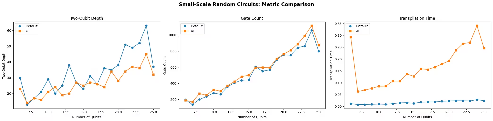
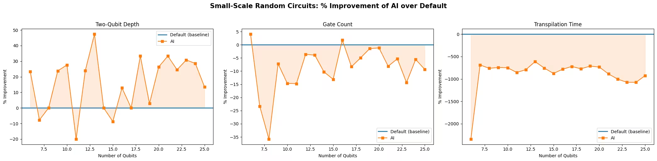
Two-qubit depth: AI-powered transpiler โดยทั่วไปผลิต Circuit ที่มี two-qubit depth ต่ำกว่า Depth เป็นหนึ่งใน metrics หลักที่ AI routing model ได้รับการฝึกให้ปรับปรุง และการปรับปรุงนี้เห็นได้ชัดในทุกขนาด Circuit แม้ว่า SABRE จะจับคู่หรือเหนือกว่าใน Circuit บางตัว

Gate count: ผลลัพธ์ใกล้เคียงกันมากในระดับนี้ โดย SABRE มีความได้เปรียบเล็กน้อยโดยรวม heuristic routing ของ SABRE ออกแบบมาเพื่อลดจำนวน SWAP gates ที่แทรกเข้า ซึ่งลด gate count โดยตรง ที่ขนาด Circuit เล็ก ความแตกต่างนั้นน้อย

เวลา transpilation: Runtime ของ SABRE แทบคงที่โดยไม่คำนึงถึงจำนวน Qubit ดังนั้นขนาด Circuit มีผลน้อยต่อเวลา transpilation ในระดับนี้ logic routing หลักของ SABRE ได้รับการปรับปรุงอย่างสูง (ส่วนใหญ่ implement ใน Rust) AI-powered transpiler ใช้เวลานานกว่าอย่างเห็นได้ชัดและปรับขนาดตาม Circuit แม้ว่าเวลาสัมบูรณ์ยังคงสมเหตุสมผลสำหรับการใช้งานแบบโต้ตอบ

ขั้นตอนที่ 3: รันโดยใช้ Qiskit primitives

เพื่อประเมินผลกระทบของการ transpilation ต่อ circuit fidelity ให้สร้าง mirror circuits จากกรณี 10-qubit และรันบน Aer simulator ด้วย noise model แบบง่าย ผลลัพธ์ที่คาดหวังของ mirror circuit คือ all-zeros bitstring เสมอ ดังนั้นความน่าจะเป็นในการวัด $|0\rangle^{\otimes n}$ แสดงให้เห็นว่าแต่ละกลยุทธ์การ transpilation รักษา fidelity ได้ดีเพียงใด

# Use the 10-qubit circuit (index where qubits == 10)
idx_10q = qubit_range_sim.index(10)

qc_10q = circuits_sim[idx_10q]
qc_default_10q, _ = transpile_with_metrics(pm_default_sim, qc_10q)

pm_ai = generate_ai_pass_manager(
    optimization_level=1,
    ai_optimization_level=3,
    backend=backend,
)
qc_ai_10q, _ = transpile_with_metrics(pm_ai, qc_10q)

tqc_methods = {
    "Default": qc_default_10q,
    "AI": qc_ai_10q,
}

print(
    f"Default: depth {qc_default_10q.depth()}, gates {qc_default_10q.size()}"
)
print(f"AI:      depth {qc_ai_10q.depth()}, gates {qc_ai_10q.size()}")

Default: depth 84, gates 280
AI:      depth 91, gates 343

# Build a simple depolarizing noise model
noise_model = NoiseModel()
noise_model.add_all_qubit_quantum_error(
    depolarizing_error(0.001, 1),
    ["sx", "x", "rz"],  # ~0.1% per 1Q gate
)
noise_model.add_all_qubit_quantum_error(
    depolarizing_error(0.01, 2),
    ["cx", "ecr"],  # ~1% per 2Q gate
)

aer_sim = AerSimulator(noise_model=noise_model)

shots = 10000
survival_probs = {}

for method, tqc in tqc_methods.items():
    mirror = build_mirror_circuit(tqc, simulate=True)

    sampler = SamplerV2(mode=aer_sim)
    job = sampler.run([mirror], shots=shots)
    counts = job.result()[0].data.meas.get_counts()

    all_zeros = "0" * mirror.num_qubits
    survival = counts.get(all_zeros, 0) / shots
    survival_probs[method] = survival
    print(
        f"{method:8s}  P(|00...0>) = {survival:.4f}  ({counts.get(all_zeros, 0)}/{shots})"
    )

Default   P(|00...0>) = 0.8460  (8460/10000)
AI        P(|00...0>) = 0.8121  (8121/10000)

เราได้รัน mirror circuits ทั้งสองผ่าน Aer simulator ด้วย depolarizing noise model แบบง่าย survival probability ซึ่งกำหนดเป็นสัดส่วนของ shots ที่คืนค่า all-zeros bitstring แสดงให้เห็นว่าแต่ละกลยุทธ์การ transpilation นำเข้า noise มากเพียงใด

ขั้นตอนที่ 4: Post-process และส่งคืนผลลัพธ์ในรูปแบบ classical ที่ต้องการ

เราดึงความน่าจะเป็นในการวัด all-zeros bitstring จากการรันทั้งสอง survival probability ที่สูงกว่าบ่งบอกถึง fidelity ที่ดีกว่า หมายความว่าการ transpilation นำเข้า noise น้อยกว่า กราฟด้านล่างแสดง complement ซึ่งก็คือ 1 - P(|0...0>) ดังนั้น bar ที่ต่ำกว่าบ่งบอกถึง fidelity ที่ดีกว่า และความแตกต่างเล็กๆ ใน error มองเห็นได้ง่ายกว่า

# Plot 1 - P(|0...0>), the probability of an erroneous (non-zero) outcome.
# A lower bar means the transpilation introduced less noise.
error_probs = {method: 1 - p for method, p in survival_probs.items()}

fig, ax = plt.subplots(figsize=(6, 4))
ax.bar(
    error_probs.keys(),
    error_probs.values(),
    color=["steelblue", "coral"],
)
ax.set_ylabel("1 - P(|0...0>)")
ax.set_title("Mirror Circuit Error (10-qubit, Aer Simulator)")
ax.set_ylim(0, 1)
plt.tight_layout()
plt.show()

ในกรณีนี้ Transpiler ค่าเริ่มต้นผลิต Circuit ที่ทั้งตื้นกว่าและเล็กกว่าสำหรับ instance 10-qubit นี้โดยเฉพาะ ดังนั้น fidelity ที่สูงกว่าจึงเป็นที่คาดไว้ ผลลัพธ์ต่อ Circuit แตกต่างกัน: ดังที่ตาราง summary ด้านบนแสดง ข้อได้เปรียบของ AI-powered transpiler อยู่ที่ two-qubit depth ที่ต่ำกว่าโดยเฉลี่ย ไม่ใช่ทุก Circuit กลยุทธ์ใดที่ให้ fidelity สูงกว่าขึ้นอยู่กับขนาดความแตกต่างของแต่ละ metric ลักษณะ noise ของฮาร์ดแวร์ และโครงสร้างของ Circuit ภายใต้ uniform depolarizing noise model จำนวน gate รวมมักมีผลกระทบโดยตรงต่อ error ที่สะสมมากกว่า depth เพียงอย่างเดียว

ตัวอย่างขนาดใหญ่บน hardware จริง

ขั้นตอนที่ 1-4

ที่นี่รายละเอียดทั้งหมดเหล่านี้ถูกนำมารวมกันเป็น workflow ที่ชัดเจนในระดับที่ใหญ่กว่า จากนั้นรันบน quantum hardware จริง

code ด้านล่างสร้าง Circuit แบบสุ่ม 25 ตัวที่มีความลึก 8 โดยจำนวน Qubit อยู่ในช่วง 26 ถึง 50 Circuit เหล่านี้จะถูก transpile ด้วยทั้งสองกลยุทธ์และเก็บ metrics เดิม จากนั้นเราสร้าง mirror circuits จากกรณี 26-qubit และส่งไปยัง Backend จริง

# -------------------------Step 1-------------------------
num_circuits_hw = 25
depth_hw = 8
qubit_range_hw = list(range(26, 51))

circuits_hw = [
    # We have only two qubit gates, as those test how well the transpiler can optimize the circuit.
    random_circuit(
        num_qubits=n,
        depth=depth_hw,
        max_operands=2,
        num_operand_distribution={2: 1},
        seed=seed + i,
    )
    for i, n in enumerate(qubit_range_hw)
]

print(
    f"Created {len(circuits_hw)} circuits with qubit counts: {qubit_range_hw}"
)

Created 25 circuits with qubit counts: [26, 27, 28, 29, 30, 31, 32, 33, 34, 35, 36, 37, 38, 39, 40, 41, 42, 43, 44, 45, 46, 47, 48, 49, 50]

# -------------------------Step 2-------------------------
pm_default = generate_preset_pass_manager(
    optimization_level=3,
    backend=backend,
    seed_transpiler=seed,
)

results_hw = []

for i, qc in enumerate(circuits_hw):
    n = qubit_range_hw[i]

    qc_default, m_default = transpile_with_metrics(pm_default, qc)

    # Create a fresh AI pass manager each iteration to avoid stale layout state
    pm_ai = generate_ai_pass_manager(
        optimization_level=1,
        ai_optimization_level=3,
        backend=backend,
    )
    qc_ai, m_ai = transpile_with_metrics(pm_ai, qc)

    results_hw.append(
        {
            "Qubits": n,
            "Depth 2Q (Default)": m_default["depth_2q"],
            "Depth 2Q (AI)": m_ai["depth_2q"],
            "Gate Count (Default)": m_default["gate_count"],
            "Gate Count (AI)": m_ai["gate_count"],
            "Time (Default)": m_default["time_s"],
            "Time (AI)": m_ai["time_s"],
        }
    )

print_summary(results_hw)

Metric        Default (mean +/- std)     AI (mean +/- std)      AI % improvement
--------------------------------------------------------------------------------
Depth 2Q              217.4 +/- 50.4        191.0 +/- 35.6      +10.9% +/- 10.7%
Gate Count         4513.3 +/- 1394.3     5227.1 +/- 1536.4       -16.4% +/- 5.8%
Time (s)                 0.1 +/- 0.0           3.5 +/- 1.5   -3588.2% +/- 643.6%

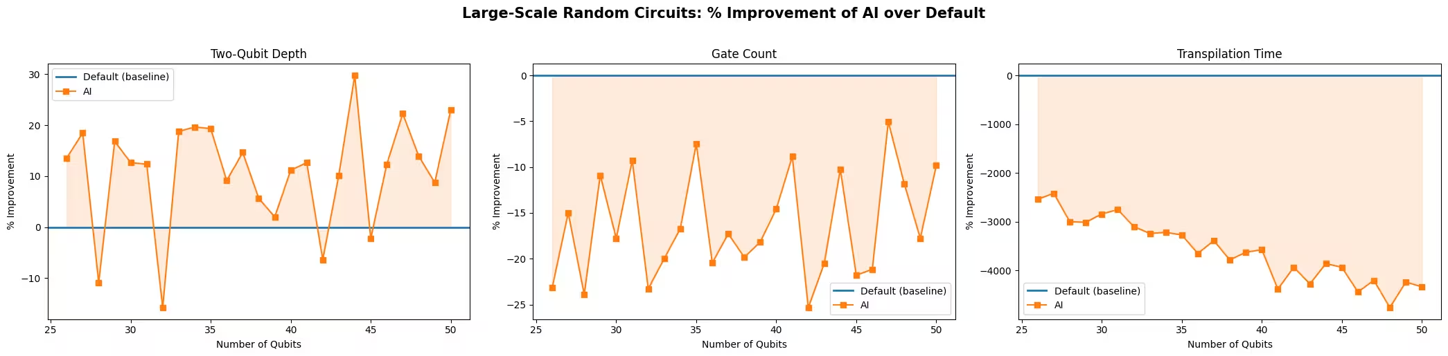
plot_metrics_and_pct(results_hw, "Large-Scale Random Circuits")

# -------------------------Step 3-------------------------
# Build mirror circuits from the 26-qubit case
idx_26q = qubit_range_hw.index(26)

qc_26q = circuits_hw[idx_26q]
qc_default_26q, _ = transpile_with_metrics(pm_default, qc_26q)

pm_ai = generate_ai_pass_manager(
    optimization_level=1,
    ai_optimization_level=3,
    backend=backend,
)
qc_ai_26q, _ = transpile_with_metrics(pm_ai, qc_26q)

mirror_default_hw = build_mirror_circuit(qc_default_26q, simulate=False)
mirror_ai_hw = build_mirror_circuit(qc_ai_26q, simulate=False)

# Re-transpile to basis gates (the inverse can introduce gates like sxdg)
pm_basis = generate_preset_pass_manager(
    optimization_level=0,
    backend=backend,
)
mirror_default_hw = pm_basis.run(mirror_default_hw)
mirror_ai_hw = pm_basis.run(mirror_ai_hw)

print(
    f"Mirror circuit (Default): depth {mirror_default_hw.depth()}, gates {mirror_default_hw.size()}"
)
print(
    f"Mirror circuit (AI):      depth {mirror_ai_hw.depth()}, gates {mirror_ai_hw.size()}"
)

# Submit to real hardware
sampler_hw = SamplerV2(mode=backend)
sampler_hw.options.environment.job_tags = ["TUT_AITI"]

shots_hw = 500000
job_hw = sampler_hw.run([mirror_default_hw, mirror_ai_hw], shots=shots_hw)
print(f"Job submitted: {job_hw.job_id()}")

Mirror circuit (Default): depth 1577, gates 9672
Mirror circuit (AI):      depth 1235, gates 11092
Job submitted: d8gt7vm6983c73dqbg0g

# -------------------------Step 4-------------------------
result_hw = job_hw.result()

survival_probs_hw = {}
for i, method in enumerate(["Default", "AI"]):
    counts = result_hw[i].data.meas.get_counts()
    mirror = [mirror_default_hw, mirror_ai_hw][i]
    all_zeros = "0" * mirror.num_qubits
    survival = counts.get(all_zeros, 0) / shots_hw
    survival_probs_hw[method] = survival
    print(
        f"{method:8s}  P(|00...0>) = {survival:.4f}  ({counts.get(all_zeros, 0)}/{shots_hw})"
    )

# Plot 1 - P(|0...0>), the probability of an erroneous (non-zero) outcome.
# A lower bar means the transpilation introduced less noise.
error_probs_hw = {method: 1 - p for method, p in survival_probs_hw.items()}

fig, ax = plt.subplots(figsize=(6, 4))
ax.bar(
    error_probs_hw.keys(),
    error_probs_hw.values(),
    color=["steelblue", "coral"],
)
ax.set_ylabel("1 - P(|0...0>)")
ax.set_title(f"Mirror Circuit Error (26-qubit, {backend.name})")
ax.set_ylim(0, 1)
plt.tight_layout()
plt.show()

Default   P(|00...0>) = 0.0005  (239/500000)
AI        P(|00...0>) = 0.0050  (2516/500000)

การวิเคราะห์ผลลัพธ์

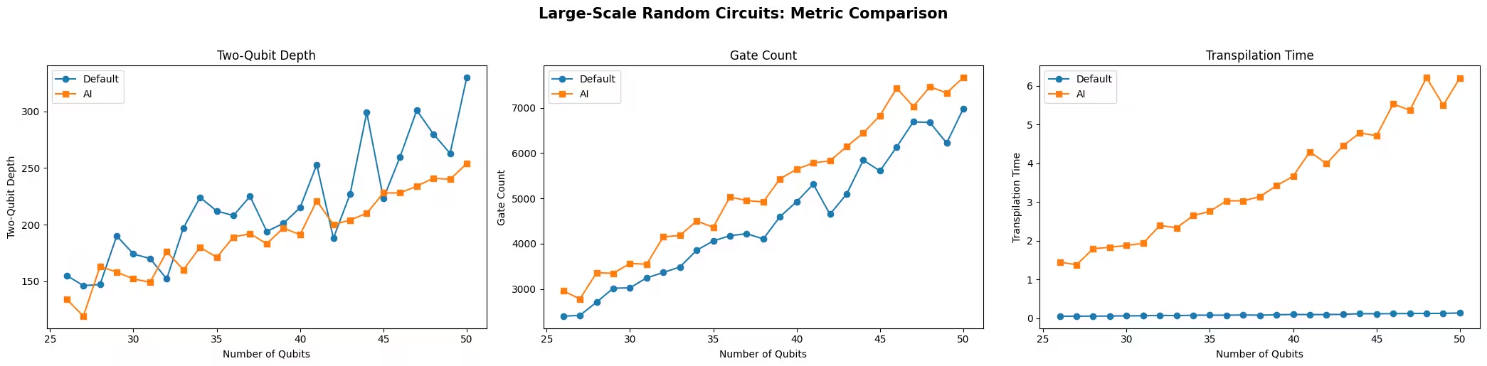
ผลลัพธ์ขนาดใหญ่ยืนยันแนวโน้มที่พบในตัวอย่างขนาดเล็ก แต่ในระดับที่ท้าทายกว่า

Two-qubit depth: AI-powered transpiler ยังคงให้ two-qubit depth ที่ต่ำกว่าอย่างเห็นได้ชัดตลอดช่วงขนาด Circuit ทั้งหมด การปรับปรุง depth เป็นหนึ่งในวัตถุประสงค์หลักที่ AI routing model ได้รับการฝึก และข้อได้เปรียบนี้ชัดเจนขึ้นที่จำนวน Qubit มากขึ้นซึ่งปัญหา routing ยากขึ้นสำหรับวิธี heuristic

Gate count: Transpiler ค่าเริ่มต้น (SABRE) ผลิต Circuit ที่มี gate น้อยกว่าอย่างสม่ำเสมอในทุกขนาด Circuit ในช่วงนี้ heuristic ของ SABRE ออกแบบมาโดยเฉพาะเพื่อลด gate count และในระดับนี้ข้อได้เปรียบชัดเจนและสม่ำเสมอ

เวลา transpilation: ช่องว่างในเวลา transpilation ขยายกว้างขึ้นในระดับใหญ่ SABRE ยังคงแทบคงที่ ในขณะที่ runtime ของ AI-powered transpiler เติบโตชันกว่า แม้ว่าเช่นนี้ runtime ของ AI-powered transpiler ยังคงใช้งานได้จริงสำหรับ workflow ส่วนใหญ่

Mirror circuit fidelity: ทั้งสองวิธีผลิต survival probabilities ต่ำกว่า 1% มากในระดับนี้ ทำให้สัญญาณที่ใช้งานได้มีน้อย ด้วยจำนวน gate รวมประมาณ 10,000 และ two-qubit depth เกิน 1,000 noise จาก depolarizing ที่สะสมตลอด mirror circuit ท่วมสัญญาณส่วนใหญ่ นี่แสดงให้เห็นข้อจำกัดสำคัญของแนวทาง mirror circuit: แม้ว่าจะเรียบง่ายและไม่ต้องการการจำลองแบบ classical แต่มันปรับขนาดได้ไม่ดีสำหรับ Circuit ที่ใหญ่หรือลึก ซึ่งทั้งสองวิธีถูกผลักให้ใกล้ noise floor และสัญญาณที่รอดเล็กน้อยถูกครอบงำด้วย error ที่สะสม

แม้ว่าผลลัพธ์เหล่านี้จะเน้นย้ำถึงประสิทธิภาพของ AI-powered transpiler แต่สิ่งสำคัญคือต้องทราบข้อจำกัดของมัน วิธีการ AI synthesis ในปัจจุบันมีให้ใช้งานเฉพาะกับ coupling maps บางอย่างเท่านั้น ซึ่งอาจจำกัดการนำไปใช้ในวงกว้าง ข้อจำกัดนี้ควรพิจารณาเมื่อประเมินการใช้งานในสถานการณ์ต่างๆ

ขั้นตอนถัดไป

คำแนะนำ

ถ้าคุณพบว่างานนี้น่าสนใจ คุณอาจสนใจเนื้อหาต่อไปนี้:

• Transpilation optimizations with SABRE
• Compilation methods for Hamiltonian simulation circuits