การปรับแต่ง Transpilation ด้วย SABRE

ประมาณเวลาการใช้งาน: 1 นาทีบนโปรเซสเซอร์ Heron r2 (หมายเหตุ: นี่เป็นเพียงการประมาณเท่านั้น เวลาจริงอาจแตกต่างกันได้)

ผลการเรียนรู้

หลังจากผ่านบทเรียนนี้ คุณจะเข้าใจ:

• วิธีการกำหนดค่าพารามิเตอร์ SABRE (layout_trials, swap_trials, max_iterations) เพื่อปรับปรุงคุณภาพ transpilation
• การแลกเปลี่ยนระหว่าง runtime ของ transpilation กับคุณภาพวงจร (depth และจำนวน gate)
• วิธีปรับแต่ง routing heuristic ของ SABRE (basic, decay, lookahead) และเปรียบเทียบประสิทธิภาพบนฮาร์ดแวร์

ข้อกำหนดเบื้องต้น

แนะนำให้คุณคุ้นเคยกับหัวข้อต่อไปนี้ก่อนเรียนบทเรียนนี้:

• Transpile circuits: ภาพรวมของ transpilation ใน Qiskit
• Transpiler stages: ขั้นตอน layout และ routing
• Configure preset pass managers: การปรับแต่ง optimization level

พื้นหลัง

Transpilation แปลง quantum circuit ให้อยู่ในรูปแบบที่เข้ากันได้กับฮาร์ดแวร์ควอนตัมที่กำหนด สองขั้นตอนสำคัญคือการเลือก qubit layout (การแมป logical qubit ไปยัง physical qubit) และ gate routing (การแทรก SWAP gate เพื่อให้ multi-qubit gate รองรับข้อจำกัดการเชื่อมต่อของอุปกรณ์)

SABRE (SWAP-Based Bidirectional heuristic search algorithm) ปรับแต่งทั้ง layout และ routing มีประสิทธิภาพเป็นพิเศษสำหรับวงจรขนาดใหญ่ (100+ qubit) บนอุปกรณ์ที่มี coupling map ซับซ้อน เช่น IBM® Heron processor SABRE ลดจำนวน SWAP gate และลด circuit depth ซึ่งช่วยปรับปรุง execution fidelity การปรับปรุงล่าสุดในอัลกอริทึม LightSABRE ช่วยลด runtime และจำนวน gate ลงไปอีก

ในบทเรียนนี้ คุณจะกำหนดค่า SabreLayout ด้วยพารามิเตอร์ต่างๆ เพื่อปรับแต่ง GHZ circuit ขนาดเล็กและสังเกต impact ต่อ execution fidelity จากนั้นเปรียบเทียบ routing heuristic ของ SABRE ที่ scale ใหญ่บนฮาร์ดแวร์จริง

ข้อกำหนด

ก่อนเริ่มบทเรียนนี้ ต้องมีสิ่งต่อไปนี้ติดตั้งอยู่:

• Qiskit SDK v2.0 หรือใหม่กว่า พร้อมรองรับ visualization
• Qiskit Runtime v0.22 หรือใหม่กว่า (pip install qiskit-ibm-runtime)
• Qiskit Aer (pip install qiskit-aer)

การตั้งค่า

# Added by doQumentation — required packages for this notebook
!pip install -q matplotlib numpy qiskit qiskit-aer qiskit-ibm-runtime

from qiskit import QuantumCircuit
from qiskit.quantum_info import SparsePauliOp
from qiskit_ibm_runtime import QiskitRuntimeService
from qiskit_ibm_runtime import EstimatorOptions
from qiskit_ibm_runtime import EstimatorV2 as Estimator
from qiskit_aer.primitives import EstimatorV2 as AerEstimator
from qiskit.transpiler.passes import (
    SabreLayout,
    SabreSwap,
    BarrierBeforeFinalMeasurements,
    StarPreRouting,
)
from qiskit.transpiler.passes.layout.vf2_layout import VF2LayoutStopReason
from qiskit.transpiler.preset_passmanagers import generate_preset_pass_manager
from qiskit.passmanager.flow_controllers import ConditionalController
import matplotlib.pyplot as plt
import numpy as np
import time

seed = 42

service = QiskitRuntimeService(
    channel="ibm_cloud",
    token="<YOUR_API_TOKEN>",  # Replace with your actual API token
    instance="<YOUR_INSTANCE_NAME>",  # Replace with your instance name if needed
)
backend = service.least_busy(operational=True, simulator=False)

print(f"Using backend: {backend.name}")

Using backend: ibm_kingston

ตัวอย่างขนาดเล็กด้วย simulator

ในส่วนนี้ ใช้ noisy simulator ที่อ้างอิง noise model จาก backend จริง เพื่อแสดงให้เห็นว่า configuration ของ SabreLayout ต่างๆ ส่งผลต่อคุณภาพ transpilation และ execution fidelity อย่างไร การใช้ qiskit_aer กับ noise model ที่ได้จากข้อมูลการสอบเทียบฮาร์ดแวร์จริงช่วยให้คุณทดสอบ transpilation โดยไม่ต้องใช้ hardware credit

ขั้นตอนที่ 1: แมป classical input ไปยังปัญหาควอนตัม

เราสร้าง star-topology GHZ circuit ที่มี 15 qubit โดย qubit แรกทำหน้าที่เป็น hub และมี CNOT gate เชื่อมต่อโดยตรงไปยัง qubit อื่นทุกตัว topology นี้สร้างปัญหา layout ที่ท้าทาย เนื่องจากไม่สามารถแมปตรงๆ ลงบน coupling map ของอุปกรณ์ได้

เรายังกำหนด ZZ operator เพื่อวัด entanglement correlation $\langle Z_0 Z_i \rangle$ ข้ามคู่ qubit

เมื่อคุณรู้โครงสร้างของวงจร

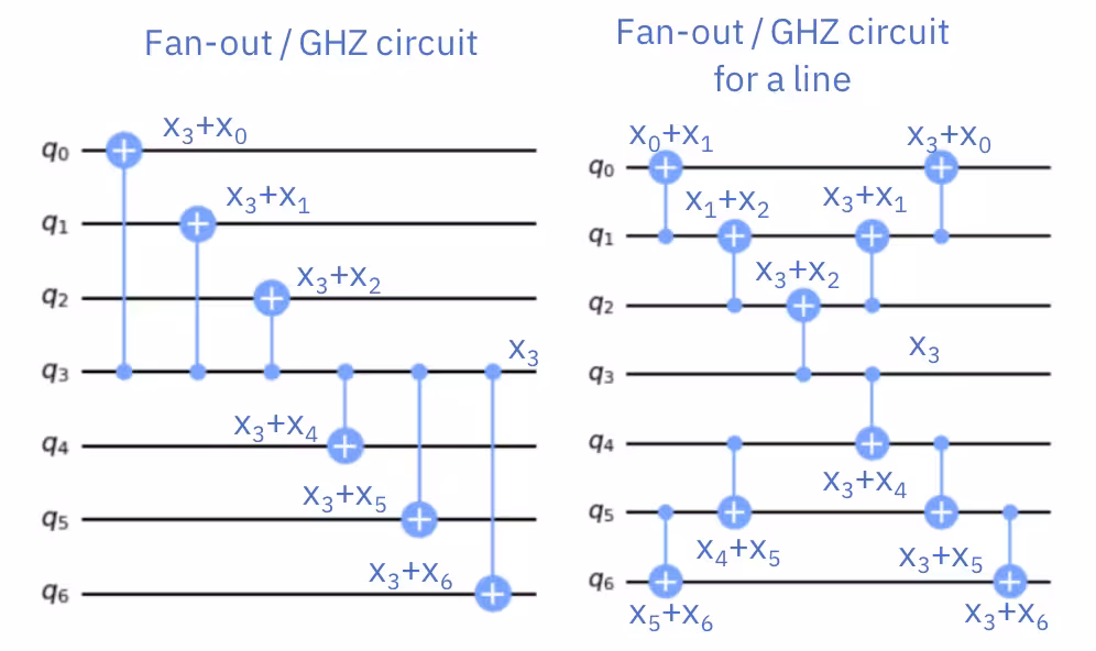
SABRE เป็นอัลกอริทึมทั่วไปและไม่มีข้อสมมติเกี่ยวกับโครงสร้างวงจร สำหรับ star-topology GHZ circuit นี้ มีการ routing ที่เหมาะสมจริงๆ ที่ทราบกัน: pass StarPreRouting ตรวจจับ star sub-circuit และเขียนใหม่เป็น linear chain ที่แมปได้โดยตรงบน backend ใดๆ ที่มี linear path ยาวพอ บทเรียนนี้เน้นที่ SABRE เพราะมันใช้ได้กับ circuit ทั่วไป แต่ถ้าคุณรู้ว่า circuit มีโครงสร้างพิเศษที่ชัดเจน การใช้ pass เฉพาะทางอย่าง StarPreRouting ก่อน routing สามารถทำได้ดีกว่า heuristic search ใดๆ

num_qubits_sim = 15

# Create star-topology GHZ circuit
qc_sim = QuantumCircuit(num_qubits_sim)
qc_sim.h(0)
for i in range(1, num_qubits_sim):
    qc_sim.cx(0, i)
qc_sim.measure_all()

# ZZ operators: Z on qubit 0 and qubit i, identity elsewhere
operator_strings_sim = [
    "Z" + "I" * i + "Z" + "I" * (num_qubits_sim - 2 - i)
    for i in range(num_qubits_sim - 1)
]
operators_sim = [SparsePauliOp(op) for op in operator_strings_sim]

ขั้นตอนที่ 2: ปรับแต่งปัญหาสำหรับการ execute บนฮาร์ดแวร์ควอนตัม

preset pass manager เริ่มต้น optimization_level=3 ใช้ SabreLayout อยู่แล้ว แต่ด้วยค่าเริ่มต้นที่อนุรักษ์นิยม เพื่อสำรวจผลของการตั้งค่าที่รุนแรงกว่า pass นั้นจะถูกแทนที่ด้วย SabreLayout แบบกำหนดเองที่ตั้งค่าสำหรับการค้นหาเชิงรุกมากขึ้น ในขณะที่ทุก pass อื่นใน layout stage ยังคงเดิม นอกจากนี้ยังเพิ่ม pass manager ที่สี่เพื่อเปรียบเทียบ: pm_star ที่ใช้ SabreLayout เริ่มต้น แต่เพิ่ม StarPreRouting ใน init stage StarPreRouting เป็น pass ที่ รู้โครงสร้าง ซึ่งตรวจจับ star sub-circuit และเขียนใหม่เป็น linear chain ก่อน routing

workflow คือ:

1. ตรวจสอบ pass manager เริ่มต้นเพื่อดูว่า SabreLayout อยู่ที่ไหนใน layout stage
2. แทนที่ pass นั้นด้วย SabreLayout instance แบบกำหนดเองโดยใช้ PassManager.replace(index, passes=...) และสร้าง pm_star variant ด้วย pm.init += StarPreRouting()
3. รัน pass manager ทั้งสี่และเปรียบเทียบ metric

configuration ทั้งสี่คือ:

Config	คำอธิบาย
pm_1 (default)	Level-3 preset เริ่มต้น (SabreLayout กับ max_iterations=4, layout_trials=20, swap_trials=20)
pm_2	SabreLayout แบบกำหนดเอง (max_iterations=4, layout_trials=200, swap_trials=200)
pm_3	SabreLayout แบบกำหนดเอง (max_iterations=8, layout_trials=200, swap_trials=200)
pm_star	Preset เริ่มต้นพร้อม StarPreRouting เพิ่มใน init stage

พารามิเตอร์สำคัญของ SABRE:

• layout_trials / swap_trials: ควบคุมจำนวน candidate layout และ routing solution ที่ SABRE สำรวจ การเพิ่มจำนวน trial ทำให้ SABRE สุ่มตัวอย่างจากพื้นที่ค้นหาที่กว้างขึ้น เพิ่มโอกาสในการหาวิธีแก้ที่ดีกว่า
• max_iterations: ควบคุมจำนวน forward-backward routing refinement cycle ที่ SABRE ทำบน candidate แต่ละตัว SABRE ปรับปรุง layout ซ้ำๆ โดยเรียนรู้จาก routing feedback ดังนั้น iteration มากขึ้นหมายถึงการปรับปรุงที่ดีกว่า

ทั้งสองมีต้นทุนที่ transpilation ใช้เวลานานขึ้น แต่วงจรที่ได้จะสั้นกว่าและใช้ gate น้อยกว่า ซึ่งช่วยลด decoherence และ gate error บนฮาร์ดแวร์จริงโดยตรง

ขั้นตอนที่ 2a: ตรวจสอบ pass manager เริ่มต้น StagedPassManager ประกอบด้วย stage ต่างๆ (init, layout, routing, translation, optimization, scheduling) แต่ละ stage เองก็เป็น PassManager การเรียก .draw() บน stage จะ render pass เป็นกราฟเพื่อให้เห็นว่า SabreLayout อยู่ที่ไหน

# Build the default pass manager (no modifications yet)
pm_1 = generate_preset_pass_manager(
    optimization_level=3, backend=backend, seed_transpiler=seed
)

# Visualize the layout stage to see where SabreLayout sits
pm_1.layout.draw()

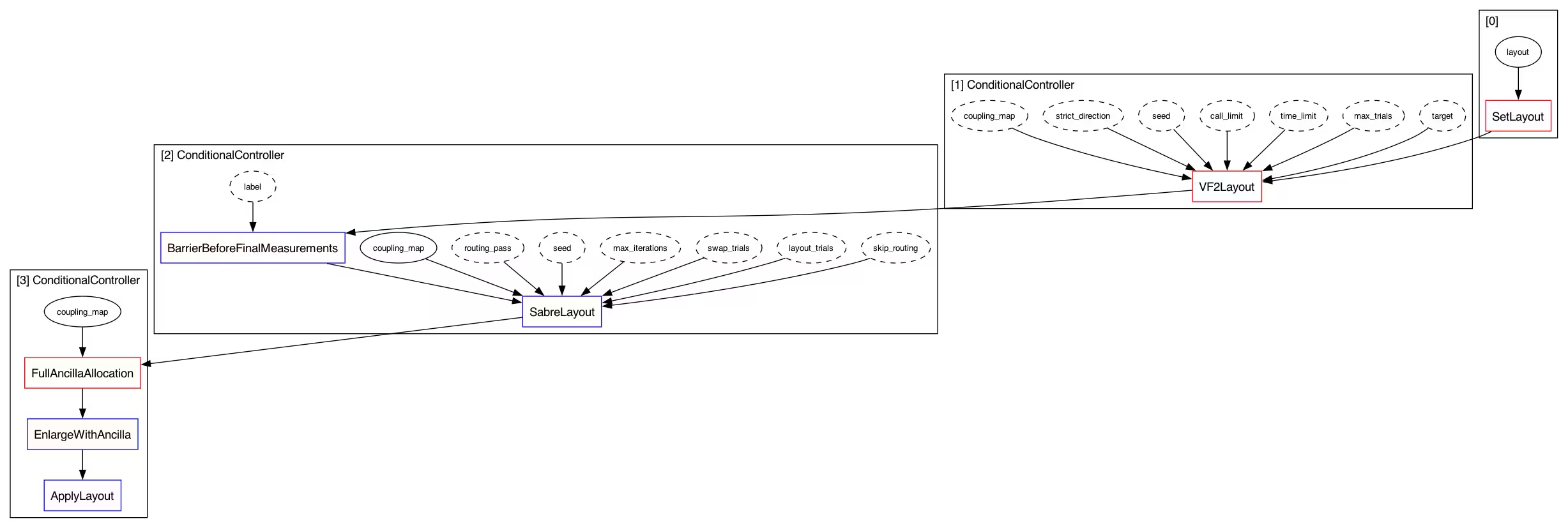
ในไดอะแกรมด้านบน pass SabreLayout ที่เราต้องการปรับแต่งอยู่ใน ConditionalController ที่ตำแหน่ง [2] ของ layout stage controller นี้ทำสองสิ่ง:

• ตรวจสอบ SabreLayout ให้รันเฉพาะเมื่อ VF2Layout ที่ [1] ไม่พบ perfect mapping (มิฉะนั้น perfect VF2 layout จะถูกเก็บไว้)
• นำหน้า SabreLayout ด้วย pass BarrierBeforeFinalMeasurements ที่ป้องกันไม่ให้ measurement ถูกจัดลำดับใหม่ระหว่าง routing ภายในของ SabreLayout

ถ้าเพียงแค่ replace(index=2, passes=sl_2) พฤติกรรมทั้งสองจะหายไป เพื่อรักษาไว้ เราห่อ SabreLayout แบบกำหนดเองของเราใน ConditionalController เดิม (พร้อม condition และ protective barrier เดิม) ก่อนสลับเข้าไป

ขั้นตอนที่ 2b: สร้าง SabreLayout pass แบบกำหนดเองและแทนที่ค่าเริ่มต้น

cmap = backend.coupling_map

# Custom SabreLayout passes with more aggressive search
sl_2 = SabreLayout(
    coupling_map=cmap,
    seed=seed,
    max_iterations=4,
    layout_trials=200,
    swap_trials=200,
)
sl_3 = SabreLayout(
    coupling_map=cmap,
    seed=seed,
    max_iterations=8,
    layout_trials=200,
    swap_trials=200,
)

# Same condition the preset uses: only run SabreLayout when VF2Layout did not
# find a perfect mapping. This preserves any perfect layout VF2 produced at [1].
def _vf2_match_not_found(property_set):
    if property_set["layout"] is None:
        return True
    return (
        property_set["VF2Layout_stop_reason"] is not None
        and property_set["VF2Layout_stop_reason"]
        is not VF2LayoutStopReason.SOLUTION_FOUND
    )

def wrap_sabre(sabre_pass):
    """Re-wrap a SabreLayout in the original ConditionalController + barrier."""
    return ConditionalController(
        [
            BarrierBeforeFinalMeasurements(
                "qiskit.transpiler.internal.routing.protection.barrier"
            ),
            sabre_pass,
        ],
        condition=_vf2_match_not_found,
    )

# Build two fresh pass managers and swap in the wrapped custom SabreLayout at index 2
pm_2 = generate_preset_pass_manager(
    optimization_level=3, backend=backend, seed_transpiler=seed
)
pm_3 = generate_preset_pass_manager(
    optimization_level=3, backend=backend, seed_transpiler=seed
)
pm_2.layout.replace(index=2, passes=wrap_sabre(sl_2))
pm_3.layout.replace(index=2, passes=wrap_sabre(sl_3))

# Build pm_star: default preset with StarPreRouting added to the init stage
pm_star = generate_preset_pass_manager(
    optimization_level=3, backend=backend, seed_transpiler=seed
)
pm_star.init += StarPreRouting()

# Visualize pm_3 after replacement (pm_2 has the same structure, only max_iterations differs)
pm_3.layout.draw()

ตำแหน่ง [2] ตอนนี้เป็น ConditionalController อีกครั้ง — มีรูปร่างเหมือนค่าเริ่มต้น แต่ SabreLayout ภายในเป็น pass แบบกำหนดเองของเรา (กับ layout_trials=200, swap_trials=200 และ max_iterations=8 สำหรับ pm_3; pm_2 เหมือนกันยกเว้น max_iterations=4) protective barrier และ _vf2_match_not_found gating ถูกรักษาไว้ ดังนั้นความแตกต่างเพียงอย่างเดียวระหว่าง pm_2/pm_3 กับ pm_1 คือ SABRE configuration เอง pm_star ใช้ SabreLayout เริ่มต้นและเพิ่มเพียง StarPreRouting ที่ท้าย init stage

ขั้นตอนที่ 2c: รัน pass manager แต่ละตัวและเปรียบเทียบ

results_sim = {}
for name, pm in [
    ("pm_1 (4,20,20)", pm_1),
    ("pm_2 (4,200,200)", pm_2),
    ("pm_3 (8,200,200)", pm_3),
    ("pm_star (default + StarPreRouting)", pm_star),
]:
    t0 = time.time()
    tqc = pm.run(qc_sim)
    elapsed = time.time() - t0
    depth = tqc.depth(lambda x: x.operation.num_qubits == 2)
    size = tqc.size()
    ops_mapped = [op.apply_layout(tqc.layout) for op in operators_sim]
    results_sim[name] = {
        "tqc": tqc,
        "ops": ops_mapped,
        "depth": depth,
        "size": size,
        "time": elapsed,
    }
    print(f"{name}: 2Q Depth {depth}, Size {size}, Time {elapsed:.2f}s")

# Print improvement relative to default (pm_1)
baseline = results_sim["pm_1 (4,20,20)"]
print("\nImprovement vs. default (pm_1):")
for name in [
    "pm_2 (4,200,200)",
    "pm_3 (8,200,200)",
    "pm_star (default + StarPreRouting)",
]:
    r = results_sim[name]
    depth_pct = (baseline["depth"] - r["depth"]) / baseline["depth"] * 100
    size_pct = (baseline["size"] - r["size"]) / baseline["size"] * 100
    print(f"  {name}: 2Q depth {depth_pct:+.1f}%, size {size_pct:+.1f}%")

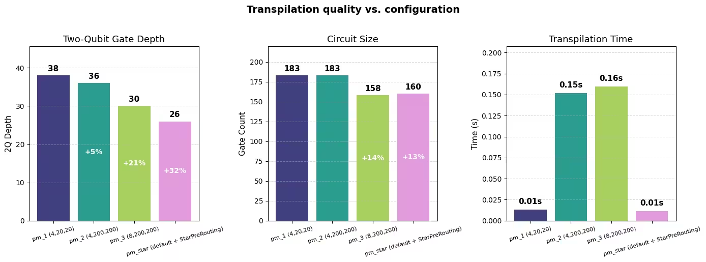
pm_1 (4,20,20): 2Q Depth 38, Size 183, Time 0.01s
pm_2 (4,200,200): 2Q Depth 36, Size 183, Time 0.15s
pm_3 (8,200,200): 2Q Depth 30, Size 158, Time 0.16s
pm_star (default + StarPreRouting): 2Q Depth 26, Size 160, Time 0.01s

Improvement vs. default (pm_1):
  pm_2 (4,200,200): 2Q depth +5.3%, size +0.0%
  pm_3 (8,200,200): 2Q depth +21.1%, size +13.7%
  pm_star (default + StarPreRouting): 2Q depth +31.6%, size +12.6%

pass manager ที่ปรับแต่งทั้งสามให้วงจรที่มี 2Q depth ต่ำกว่าค่าเริ่มต้น SABRE configuration แบบรุนแรง (pm_2 และ pm_3) แลกเวลา transpilation ที่นานกว่าเพื่อค้นหาที่กว้างขึ้น ในขณะที่ pm_star ใช้ประโยชน์จากโครงสร้าง star ของวงจรและผลิตผลลัพธ์ที่ตื้นกว่าโดยไม่ต้องจ่ายต้นทุน transpilation เพิ่มเติม ผลกำไรที่แน่นอนจะแตกต่างกันในแต่ละรัน แต่แนวโน้มทั่วไปสอดคล้องกัน: SABRE trial และ iteration มากขึ้นทำให้ heuristic ค้นหาพื้นที่กว้างขึ้น และ pass ที่รู้โครงสร้างอย่าง StarPreRouting สามารถข้ามการค้นหานั้นได้เลยเมื่อรูปร่างวงจรตรงกัน

แม้ที่ scale เล็กนี้ (15 qubit) ก็มีพื้นที่สำหรับการปรับปรุงเพียงพอที่ทั้งสามวิธีเอาชนะค่าเริ่มต้น ด้วยวงจรขนาดใหญ่ขึ้น (100+ qubit) พื้นที่ค้นหาเติบโตอย่างมาก และประโยชน์ของทั้งการเพิ่ม trial และ pass ที่รู้โครงสร้างจะเด่นชัดยิ่งขึ้นมาก ดังที่ส่วน large-scale จะแสดง

pm_names = list(results_sim.keys())
depths = [results_sim[n]["depth"] for n in pm_names]
sizes = [results_sim[n]["size"] for n in pm_names]
times = [results_sim[n]["time"] for n in pm_names]
colors = ["#404080", "#2a9d8f", "#a8d05e", "#e29bdd"]
x = np.arange(len(pm_names))

fig, axs = plt.subplots(1, 3, figsize=(14, 5))

# 2Q Depth
bars = axs[0].bar(x, depths, color=colors)
axs[0].set_ylabel("2Q Depth", fontsize=11)
axs[0].set_title("Two-Qubit Gate Depth", fontsize=13)
axs[0].set_ylim(0, max(depths) * 1.2)
for bar, val in zip(bars, depths):
    axs[0].text(
        bar.get_x() + bar.get_width() / 2,
        bar.get_height() + max(depths) * 0.02,
        str(val),
        ha="center",
        va="bottom",
        fontsize=11,
        fontweight="bold",
    )
for i in range(1, len(depths)):
    pct = (depths[0] - depths[i]) / depths[0] * 100
    if pct != 0:
        axs[0].text(
            bars[i].get_x() + bars[i].get_width() / 2,
            bars[i].get_height() / 2,
            f"{pct:+.0f}%",
            ha="center",
            va="center",
            fontsize=10,
            color="white",
            fontweight="bold",
        )

# Size
bars = axs[1].bar(x, sizes, color=colors)
axs[1].set_ylabel("Gate Count", fontsize=11)
axs[1].set_title("Circuit Size", fontsize=13)
axs[1].set_ylim(0, max(sizes) * 1.2)
for bar, val in zip(bars, sizes):
    axs[1].text(
        bar.get_x() + bar.get_width() / 2,
        bar.get_height() + max(sizes) * 0.02,
        str(val),
        ha="center",
        va="bottom",
        fontsize=11,
        fontweight="bold",
    )
for i in range(1, len(sizes)):
    pct = (sizes[0] - sizes[i]) / sizes[0] * 100
    if abs(pct) > 0.1:
        axs[1].text(
            bars[i].get_x() + bars[i].get_width() / 2,
            bars[i].get_height() / 2,
            f"{pct:+.0f}%",
            ha="center",
            va="center",
            fontsize=10,
            color="white",
            fontweight="bold",
        )

# Time
bars = axs[2].bar(x, times, color=colors)
axs[2].set_ylabel("Time (s)", fontsize=11)
axs[2].set_title("Transpilation Time", fontsize=13)
axs[2].set_ylim(0, max(times) * 1.3)
for bar, val in zip(bars, times):
    axs[2].text(
        bar.get_x() + bar.get_width() / 2,
        bar.get_height() + max(times) * 0.03,
        f"{val:.2f}s",
        ha="center",
        va="bottom",
        fontsize=11,
        fontweight="bold",
    )

for ax in axs:
    ax.set_xticks(x)
    ax.set_xticklabels(pm_names, fontsize=8, rotation=15)
    ax.grid(axis="y", linestyle="--", alpha=0.5)

plt.suptitle(
    "Transpilation quality vs. configuration",
    fontsize=14,
    fontweight="bold",
    y=1.02,
)
plt.tight_layout()
plt.show()

ขั้นตอนที่ 3: Execute ด้วย Qiskit primitives

เรารัน circuit ที่ transpiled แต่ละตัว 10 ครั้ง โดยใช้ Aer EstimatorV2 กับ noise model ที่ได้จาก backend จริง เนื่องจากผลลัพธ์ noisy simulation แตกต่างกันในแต่ละรัน การเฉลี่ยหลายรันให้การประมาณ fidelity ที่เชื่อถือได้มากขึ้นและช่วยวัด statistical uncertainty ด้วย error bar

# Create a noisy estimator from the real backend's noise model
noisy_estimator = AerEstimator.from_backend(backend)

num_runs = 10
# sim_all_runs[name] = list of arrays, one per run
sim_all_runs = {name: [] for name in results_sim}

for run in range(num_runs):
    for name, r in results_sim.items():
        job = noisy_estimator.run([(r["tqc"], r["ops"])])
        evs = list(job.result()[0].data.evs)
        sim_all_runs[name].append(evs)
    print(f"Run {run + 1}/{num_runs} done")

# Compute mean and std across runs for each config
sim_stats = {}
for name in results_sim:
    all_evs = np.array(sim_all_runs[name])  # shape (num_runs, num_operators)
    sim_stats[name] = {
        "mean": np.mean(all_evs, axis=0),
        "std": np.std(all_evs, axis=0),
        "overall_mean": np.mean(all_evs),
        "overall_std": np.std(
            np.mean(all_evs, axis=1)
        ),  # std of per-run averages
    }
    print(
        f"{name}: mean fidelity = {sim_stats[name]['overall_mean']:.4f} +/- {sim_stats[name]['overall_std']:.4f}"
    )

Run 1/10 done
Run 2/10 done
Run 3/10 done
Run 4/10 done
Run 5/10 done
Run 6/10 done
Run 7/10 done
Run 8/10 done
Run 9/10 done
Run 10/10 done
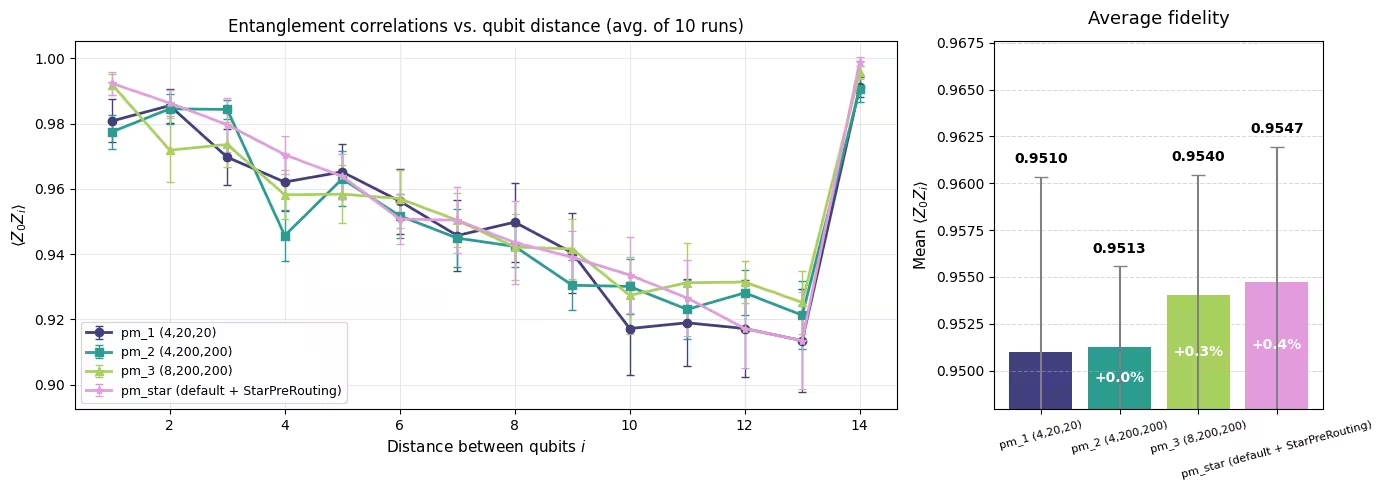
pm_1 (4,20,20): mean fidelity = 0.9510 +/- 0.0094
pm_2 (4,200,200): mean fidelity = 0.9513 +/- 0.0043
pm_3 (8,200,200): mean fidelity = 0.9540 +/- 0.0065
pm_star (default + StarPreRouting): mean fidelity = 0.9547 +/- 0.0072

เนื่องจากนี่เป็นวงจรขนาดเล็ก ค่า fidelity อยู่ค่อนข้างใกล้กันในทุก configuration วงจรสั้นพอที่ hardware noise ไม่ลงโทษแม้แต่เวอร์ชันที่ optimized น้อยที่สุดอย่างหนัก Mean fidelity โดยกว้างๆ ตาม 2Q depth: pm_3 และ pm_star สองวงจรที่ตื้นที่สุด ให้ fidelity สูงสุดและเสมอกันในระดับ error bar pm_2 เป็นตัวอย่างที่ขัดแย้ง: แม้ว่า 2Q depth ต่ำกว่า pm_1 แต่ mean fidelity ก็ต่ำกว่าเล็กน้อยเช่นกัน ซึ่งเป็นการเตือนว่าความสัมพันธ์ระหว่าง depth กับ fidelity เป็นแบบสถิติ ไม่ใช่แบบกำหนดแน่นอน qubit เฉพาะที่ layout เลือกและการสอบเทียบ qubit เหล่านั้น ณ เวลารันก็มีความสำคัญเช่นกัน

ขั้นตอนที่ 4: Post-process และคืนผลในรูปแบบ classical ที่ต้องการ

ต่อไป plot entanglement correlation $\langle Z_0 Z_i \rangle$ เป็นฟังก์ชันของระยะห่าง qubit พร้อมกับ mean correlation เป็น fidelity metric เดียว ในกรณีอุดมคติ (ไม่มี noise) correlation ทั้งหมดจะเป็น 1 ด้วย noise จริง gate เพิ่มเติมแต่ละตัวนำ error เข้ามาและแต่ละ time step เพิ่มเติมทำให้ decoherence ดังนั้นวงจร transpiled ที่มี depth ต่ำกว่าและ gate น้อยกว่า (โดยเฉพาะ two-qubit gate) ควรรักษา entanglement ได้ดีกว่า

data_sim = list(range(1, len(operators_sim) + 1))
markers = ["o", "s", "^", "*"]
colors_line = ["#404080", "#2a9d8f", "#a8d05e", "#e29bdd"]

fig, (ax1, ax2) = plt.subplots(
    1, 2, figsize=(14, 5), gridspec_kw={"width_ratios": [2.5, 1]}
)

# Left: correlations vs distance with error bars (mean +/- 1 std)
for (name, stats), marker, color in zip(
    sim_stats.items(), markers, colors_line
):
    ax1.errorbar(
        data_sim,
        stats["mean"],
        yerr=stats["std"],
        marker=marker,
        label=name,
        color=color,
        linewidth=2,
        capsize=3,
        capthick=1,
        elinewidth=1,
    )

ax1.set_xlabel("Distance between qubits $i$", fontsize=11)
ax1.set_ylabel(r"$\langle Z_0 Z_i \rangle$", fontsize=11)
ax1.set_title(
    "Entanglement correlations vs. qubit distance (avg. of 10 runs)",
    fontsize=12,
)
ax1.legend(fontsize=9)
ax1.grid(alpha=0.3)

# Right: mean correlation bar chart with error bars
names = list(sim_stats.keys())
means = [sim_stats[n]["overall_mean"] for n in names]
stds = [sim_stats[n]["overall_std"] for n in names]
x_bar = np.arange(len(names))
bars = ax2.bar(
    x_bar, means, yerr=stds, color=colors_line, capsize=5, ecolor="gray"
)
ax2.set_ylabel(r"Mean $\langle Z_0 Z_i \rangle$", fontsize=11)
ax2.set_title("Average fidelity", fontsize=13, pad=12)
y_range = max(means) - min(means) if max(means) != min(means) else 0.01
# Top of ylim accounts for the bar height + std error bar + headroom for the value label
y_top = max(m + s for m, s in zip(means, stds)) + y_range * 1.5
ax2.set_ylim(min(means) - y_range * 0.8, y_top)
for bar, val, std in zip(bars, means, stds):
    ax2.text(
        bar.get_x() + bar.get_width() / 2,
        bar.get_height() + std + y_range * 0.15,
        f"{val:.4f}",
        ha="center",
        va="bottom",
        fontsize=10,
        fontweight="bold",
    )
# Annotate % change vs pm_1
baseline_mean = means[0]
for i in range(1, len(means)):
    pct = (means[i] - baseline_mean) / baseline_mean * 100
    if abs(pct) > 0.01:
        mid_y = (means[i] + ax2.get_ylim()[0]) / 2
        ax2.text(
            bars[i].get_x() + bars[i].get_width() / 2,
            mid_y,
            f"{pct:+.1f}%",
            ha="center",
            va="center",
            fontsize=10,
            color="white",
            fontweight="bold",
        )
ax2.set_xticks(x_bar)
ax2.set_xticklabels(names, fontsize=8, rotation=15)
ax2.grid(axis="y", linestyle="--", alpha=0.5)

fig.tight_layout()
plt.show()

ผลลัพธ์แสดงความสัมพันธ์ที่ชัดเจนระหว่างคุณภาพ transpilation และ execution fidelity พร้อมข้อสังเกตที่มีประโยชน์:

• pm_1 (default): Baseline ด้วยเพียง 20 trial และสี่ iteration SABRE มีพื้นที่จำกัดในการ optimize ส่งผลให้วงจรที่ลึกที่สุดในบรรดาวงจร SABRE เท่านั้น
• pm_2 (more trials): การสำรวจ candidate มากกว่าสิบเท่าพบ layout ที่ตื้นกว่าเล็กน้อย แต่ mean fidelity ค่อนข้างคงที่ (และอาจต่ำกว่า baseline ได้ภายใน noise) เนื่องจากผลกำไร depth มีขนาดเล็กที่ scale นี้
• pm_3 (more trials + more iterations): การเพิ่ม max_iterations เป็น 8 ให้ SABRE มี refinement cycle มากขึ้น ผลิตวงจร SABRE-only ที่ตื้นที่สุดและ mean fidelity สูงสุดในการเปรียบเทียบ
• pm_star (default + StarPreRouting): เพิ่ม StarPreRouting ใน init stage ของ preset เริ่มต้นที่ไม่เปลี่ยนแปลง การ rewrite ที่รู้โครงสร้างยุบ star เป็น linear chain ที่ transpiler ที่เหลือแมปลงบน linear path ของอุปกรณ์ ผลิตวงจรที่ตื้นที่สุดโดยรวม (ดีกว่า pm_3 เล็กน้อย) และเสมอกับ pm_3 ใน fidelity ภายใน error bar ทำได้ด้วยเวลา transpilation เดียวกับค่าเริ่มต้น เนื่องจาก rewrite แทบไม่มีต้นทุนเทียบกับ stochastic search ของ SABRE

โปรดสังเกตว่าการเพิ่ม max_iterations ไม่ได้มีผลบวกเสมอไป ในกรณีนี้ช่วยได้อย่างมีนัยสำคัญ แต่สำหรับวงจรหรือ backend อื่น iteration เพิ่มเติมอาจไม่ให้การปรับปรุงเพิ่มเติม หรืออาจทำให้แย่ลงเล็กน้อยเนื่องจาก over-optimization ของ local minimum โดยทั่วไป ควรเพิ่ม layout_trials และ swap_trials มากที่สุดเท่าที่งบเวลาอนุญาต เนื่องจาก trial มากขึ้นเพิ่มโอกาสในการหา layout ที่ดีกว่าเสมอ การเพิ่ม max_iterations ควรทดสอบแต่ควรตรวจสอบสำหรับกรณีการใช้งานเฉพาะของคุณ Pass เฉพาะทางอย่าง StarPreRouting มีจิตวิญญาณคล้ายกันแต่ขึ้นอยู่กับวงจรมากกว่า: ช่วยได้เฉพาะเมื่อวงจรมีโครงสร้างที่มันกำหนดเป้าหมายจริงๆ ผลกำไรมีขนาดใหญ่เมื่อใช้ได้และเป็นศูนย์มิฉะนั้น แต่แทบไม่มีต้นทุนในการลอง

ตัวอย่างขนาดใหญ่บนฮาร์ดแวร์

นอกจากการปรับจำนวน trial แล้ว SABRE ยังรองรับการปรับแต่ง routing heuristic SABRE มี heuristic สามแบบ:

• basic: วิธี greedy ง่ายๆ ที่เลือก swap ที่ลดระยะทางทันทีไปยัง gate ถัดไป
• decay (default): ถ่วงน้ำหนัก qubit แบบ dynamic ตามกิจกรรมล่าสุด ไม่สนับสนุนการ swap ซ้ำๆ บน qubit เดิม
• lookahead: ประเมิน routing cost ในอนาคตโดยมองล่วงหน้าไปยัง gate ที่กำลังจะมาถึง อาจพบ swap sequence ที่ดีกว่า

ในการใช้ heuristic แบบกำหนดเอง ให้สร้าง SabreSwap pass และเชื่อมต่อกับ SabreLayout ผ่านพารามิเตอร์ routing_pass

pass manager ที่สี่ถูกเพิ่มในการเปรียบเทียบ: pm_star_hw ที่ใช้การตั้งค่า SabreLayout/SabreSwap เริ่มต้น แต่เพิ่ม StarPreRouting ใน init stage ที่ scale นี้ (100 qubit) การค้นหา SABRE ยากขึ้น และการ rewrite จาก star เป็น linear chain กลายเป็นข้อได้เปรียบที่ชัดเจน เพราะ Heron processor มี linear path ยาวพอที่จะรองรับวงจรที่ได้

ที่นี่เราเปรียบเทียบ SABRE heuristic ทั้งสามบวก StarPreRouting ที่ scale บน GHZ circuit 100-qubit เรารัน layout trial หลายครั้งด้วย seed ต่างกันสำหรับ SABRE configuration เลือกวงจร transpiled ที่ดีที่สุดจากแต่ละตัว และส่งทั้งหมดไปยังฮาร์ดแวร์จริงพร้อมกับผลลัพธ์ StarPreRouting

ขั้นตอน 1-4 รวมไว้ใน code block เดียว

ที่นี่ workflow ทั้งหมดถูกรวมไว้ที่ scale ที่ใหญ่ขึ้น เมื่อใช้ SabreSwap เป็น routing_pass สำหรับ SabreLayout จะมีเพียง layout trial เดียวต่อการเรียกหนึ่งครั้ง ดังนั้น code cell ต่อไปนี้จะวน loop ผ่าน seed เพื่อสำรวจ layout space

เราใช้ helper wrap_sabre เดิมที่กำหนดใน small-scale Step 2 (ด้านบน) และเพิ่ม helper wrap_routing ที่คล้ายกัน เพราะ routing stage ที่ index [1] ก็เป็น ConditionalController([BarrierBeforeFinalMeasurements, routing_pass], ...) เช่นกัน — การแทนที่แบบเปล่าจะลบ protective barrier และ _swap_condition gating ออกเช่นเดียวกัน

# -------------------------Step 1-------------------------

num_qubits = 100

# Create star-topology GHZ circuit
qc = QuantumCircuit(num_qubits)
qc.h(0)
for i in range(1, num_qubits):
    qc.cx(0, i)
qc.measure_all()

# ZZ operators
operator_strings = [
    "Z" + "I" * i + "Z" + "I" * (num_qubits - 2 - i)
    for i in range(num_qubits - 1)
]
operators = [SparsePauliOp(op) for op in operator_strings]

# -------------------------Step 2-------------------------

num_seeds = 10
seed_list = [seed + i for i in range(num_seeds)]
swap_trials = 200

# The default routing[1] is a ConditionalController([barrier, routing_pass],
# condition=_swap_condition); we re-wrap so the new routing pass keeps the
# protective barrier and is skipped when routing isn't needed (matches the preset).
def _swap_condition(property_set):
    return not property_set["routing_not_needed"]

def wrap_routing(routing_pass):
    return ConditionalController(
        [
            BarrierBeforeFinalMeasurements(
                "qiskit.transpiler.internal.routing.protection.barrier"
            ),
            routing_pass,
        ],
        condition=_swap_condition,
    )

heuristic_results = {}

# Three SABRE heuristics, swept over seeds
for heuristic in ["basic", "decay", "lookahead"]:
    trials = []
    for s in seed_list:
        sr = SabreSwap(
            coupling_map=cmap, heuristic=heuristic, trials=swap_trials, seed=s
        )
        sl = SabreLayout(coupling_map=cmap, routing_pass=sr, seed=s)
        pm = generate_preset_pass_manager(
            optimization_level=3, backend=backend, seed_transpiler=s
        )
        # Re-wrap each custom pass in its original ConditionalController + barrier
        # (wrap_sabre is defined in the small-scale Step 2 cell above).
        pm.layout.replace(index=2, passes=wrap_sabre(sl))
        pm.routing.replace(index=1, passes=wrap_routing(sr))

        t0 = time.time()
        tqc = pm.run(qc)
        elapsed = time.time() - t0
        depth = tqc.depth(lambda x: x.operation.num_qubits == 2)
        size = tqc.size()
        trials.append(
            {
                "tqc": tqc,
                "depth": depth,
                "size": size,
                "time": elapsed,
                "seed": s,
            }
        )

    heuristic_results[heuristic] = trials

# Default preset + StarPreRouting in init, also swept over seeds for a fair comparison
star_trials = []
for s in seed_list:
    pm_star_hw = generate_preset_pass_manager(
        optimization_level=3, backend=backend, seed_transpiler=s
    )
    pm_star_hw.init += StarPreRouting()

    t0 = time.time()
    tqc = pm_star_hw.run(qc)
    elapsed = time.time() - t0
    depth = tqc.depth(lambda x: x.operation.num_qubits == 2)
    size = tqc.size()
    star_trials.append(
        {
            "tqc": tqc,
            "depth": depth,
            "size": size,
            "time": elapsed,
            "seed": s,
        }
    )
heuristic_results["StarPreRouting"] = star_trials

# Print summary for each entry
for label in ["basic", "decay", "lookahead", "StarPreRouting"]:
    trials = heuristic_results[label]
    depths = [t["depth"] for t in trials]
    sizes = [t["size"] for t in trials]
    best = min(trials, key=lambda t: t["depth"])
    print(f"{label}:")
    print(
        f"  2Q depth: min: {min(depths)}, mean: {np.mean(depths):.1f}, std: {np.std(depths):.1f}"
    )
    print(
        f"  size    : min: {min(sizes)}, mean: {np.mean(sizes):.1f}, std: {np.std(sizes):.1f}"
    )
    print(
        f"  best seed: {best['seed']} (2Q depth={best['depth']}, size={best['size']})"
    )

basic:
  2Q depth: min: 524, mean: 570.5, std: 39.9
  size    : min: 3819, mean: 4227.1, std: 360.6
  best seed: 51 (2Q depth=524, size=3852)
decay:
  2Q depth: min: 387, mean: 436.4, std: 41.7
  size    : min: 2687, mean: 3183.1, std: 459.3
  best seed: 45 (2Q depth=387, size=2786)
lookahead:
  2Q depth: min: 364, mean: 424.6, std: 36.5
  size    : min: 2335, mean: 3014.6, std: 388.1
  best seed: 51 (2Q depth=364, size=2485)
StarPreRouting:
  2Q depth: min: 196, mean: 196.0, std: 0.0
  size    : min: 1151, mean: 1151.0, std: 0.0
  best seed: 42 (2Q depth=196, size=1151)

hw_colors = {
    "basic": "#ff7f0e",
    "decay": "#d62728",
    "lookahead": "#1f77b4",
    "StarPreRouting": "#2a9d8f",
}

fig, (ax1, ax2) = plt.subplots(1, 2, figsize=(13, 5))

for label in ["basic", "decay", "lookahead", "StarPreRouting"]:
    trials = heuristic_results[label]
    depths = [t["depth"] for t in trials]
    sizes = [t["size"] for t in trials]
    seeds = [t["seed"] for t in trials]
    color = hw_colors[label]

    ax1.scatter(
        seeds,
        depths,
        label=label,
        color=color,
        alpha=0.8,
        edgecolor="k",
        s=60,
    )
    ax1.axhline(np.mean(depths), color=color, linestyle="--", alpha=0.5)

    ax2.scatter(
        seeds,
        sizes,
        label=label,
        color=color,
        alpha=0.8,
        edgecolor="k",
        s=60,
    )
    ax2.axhline(np.mean(sizes), color=color, linestyle="--", alpha=0.5)

ax1.set_xlabel("Seed", fontsize=11)
ax1.set_ylabel("2Q Depth", fontsize=11)
ax1.set_title("Two-Qubit Gate Depth per Seed", fontsize=13)
ax1.legend(fontsize=10)
ax1.grid(alpha=0.3)

ax2.set_xlabel("Seed", fontsize=11)
ax2.set_ylabel("Gate Count", fontsize=11)
ax2.set_title("Circuit Size per Seed", fontsize=13)
ax2.legend(fontsize=10)
ax2.grid(alpha=0.3)

plt.suptitle(
    "Transpilation variability across seeds: SABRE heuristics vs. StarPreRouting",
    fontsize=14,
    fontweight="bold",
    y=1.02,
)
plt.tight_layout()
plt.show()

# Summary comparison
for label in ["basic", "decay", "lookahead", "StarPreRouting"]:
    best = min(heuristic_results[label], key=lambda t: t["depth"])
    print(
        f"{label}: best 2Q depth={best['depth']}, size={best['size']} (seed={best['seed']})"
    )

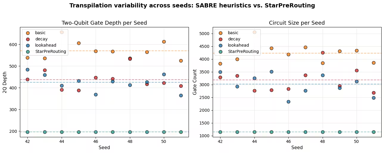
basic: best 2Q depth=524, size=3852 (seed=51)
decay: best 2Q depth=387, size=2786 (seed=45)
lookahead: best 2Q depth=364, size=2485 (seed=51)
StarPreRouting: best 2Q depth=196, size=1151 (seed=42)

# -------------------------Step 3: Execute on hardware-------------------------

best_circuits = {}
for label in ["basic", "decay", "lookahead", "StarPreRouting"]:
    best_circuits[label] = min(
        heuristic_results[label], key=lambda t: t["depth"]
    )
    b = best_circuits[label]
    print(f"Best {label}: 2Q depth={b['depth']}, size={b['size']}")

options = EstimatorOptions()
options.resilience_level = 2
options.dynamical_decoupling.enable = True
options.dynamical_decoupling.sequence_type = "XY4"
estimator = Estimator(backend, options=options)

hw_jobs = {}
hw_ops = {}
for label, best in best_circuits.items():
    hw_ops[label] = [op.apply_layout(best["tqc"].layout) for op in operators]
    hw_jobs[label] = estimator.run([(best["tqc"], hw_ops[label])])
    print(f"{label} job: {hw_jobs[label].job_id()}")
estimator.options.environment.job_tags = ["TUT_TOWS"]

hw_results = {}
for label, job in hw_jobs.items():
    hw_results[label] = job.result()[0]
    print(f"{label} job done")

Best basic: 2Q depth=524, size=3852
Best decay: 2Q depth=387, size=2786
Best lookahead: 2Q depth=364, size=2485
Best StarPreRouting: 2Q depth=196, size=1151
basic job: d81q5tnoha1c73bknprg
decay job: d81q5tugbeec73aktopg
lookahead job: d81q5to0bvlc73d1epe0
StarPreRouting job: d81q5u7tjchs73bn82hg
basic job done
decay job done
lookahead job done
StarPreRouting job done

# -------------------------Step 4: Post-process-------------------------

data = list(range(1, len(operators) + 1))
hw_markers = {
    "basic": "D",
    "decay": "o",
    "lookahead": "s",
    "StarPreRouting": "*",
}
hw_labels = ["basic", "decay", "lookahead", "StarPreRouting"]

fig, (ax1, ax2) = plt.subplots(
    1, 2, figsize=(14, 5), gridspec_kw={"width_ratios": [2.5, 1]}
)

# Left: correlations vs distance
for label in hw_labels:
    evs = list(hw_results[label].data.evs)
    b = best_circuits[label]
    ax1.plot(
        data,
        evs,
        marker=hw_markers[label],
        color=hw_colors[label],
        linewidth=2,
        label=f"{label} (2Q depth={b['depth']}, size={b['size']})",
        markersize=5 if label == "StarPreRouting" else 4,
    )

ax1.set_xlabel("Distance between qubits $i$", fontsize=11)
ax1.set_ylabel(r"$\langle Z_0 Z_i \rangle$", fontsize=11)
ax1.set_title(
    "Entanglement correlations vs. qubit distance (hardware)", fontsize=12
)
ax1.legend(fontsize=9)
ax1.grid(alpha=0.3)

# Right: mean fidelity bar chart
hw_means = [np.mean(list(hw_results[label].data.evs)) for label in hw_labels]
hw_bar_colors = [hw_colors[label] for label in hw_labels]
x_bar = np.arange(len(hw_labels))
bars = ax2.bar(x_bar, hw_means, color=hw_bar_colors)
ax2.set_ylabel(r"Mean $\langle Z_0 Z_i \rangle$", fontsize=11)
ax2.set_title("Average fidelity", fontsize=13)
y_range = (
    max(hw_means) - min(hw_means) if max(hw_means) != min(hw_means) else 0.01
)
ax2.set_ylim(min(hw_means) - y_range * 0.2, max(hw_means) + y_range * 0.15)
for bar, val in zip(bars, hw_means):
    ax2.text(
        bar.get_x() + bar.get_width() / 2,
        bar.get_height() + y_range * 0.05,
        f"{val:.4f}",
        ha="center",
        va="bottom",
        fontsize=11,
        fontweight="bold",
    )
ax2.set_xticks(x_bar)
ax2.set_xticklabels(hw_labels, fontsize=9, rotation=15)
ax2.grid(axis="y", linestyle="--", alpha=0.5)

fig.tight_layout()
plt.show()

print("\nMean fidelity:")
for label, m in zip(hw_labels, hw_means):
    print(f"  {label}: {m:.4f}")

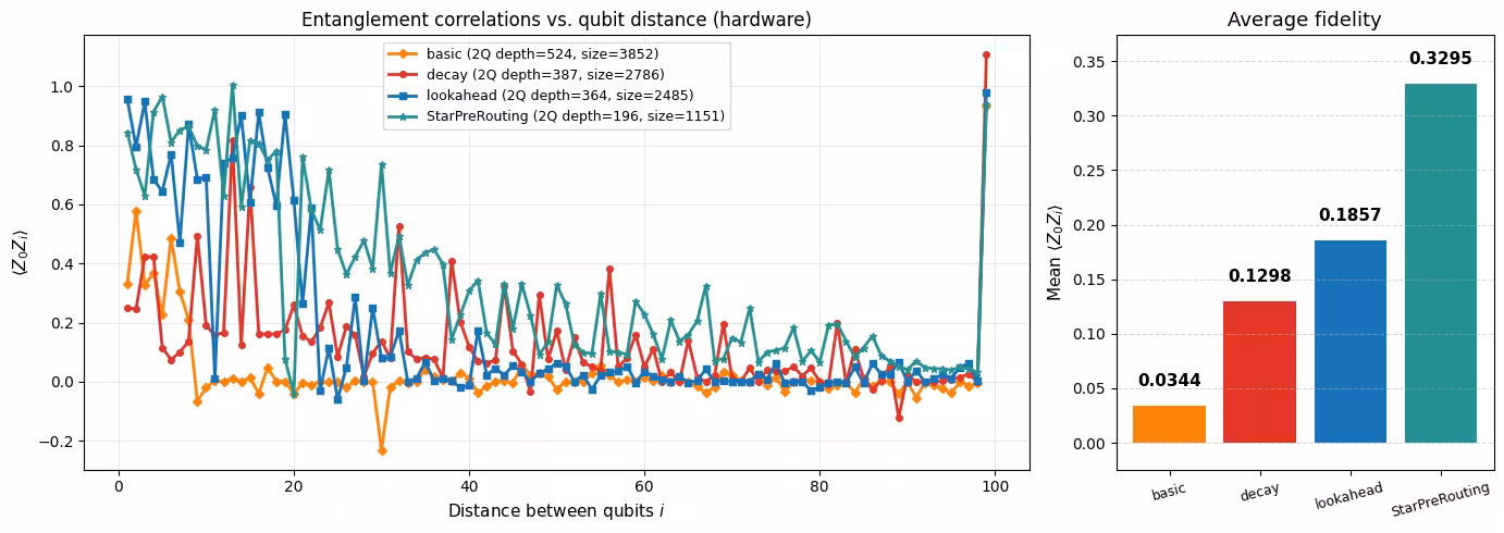
Mean fidelity:
  basic: 0.0344
  decay: 0.1298
  lookahead: 0.1857
  StarPreRouting: 0.3295

การวิเคราะห์

scatter plot แสดงความแปรผันอย่างมีนัยสำคัญข้าม seed สำหรับ SABRE heuristic ทั้งสามแบบ ซึ่งเน้นย้ำความสำคัญของการรัน layout trial หลายครั้งแทนที่จะพึ่งพา transpilation เพียงครั้งเดียว เส้น StarPreRouting แทบแบนราบข้าม seed เนื่องจาก rewrite จาก star เป็น linear chain เป็นแบบ deterministic ตามโครงสร้าง; SABRE routing ที่ตามมาจึงมีอิสระน้อยมากบน linear chain ดังนั้น seed แทบไม่มีผลต่อ depth หรือ size สุดท้าย

จากผลลัพธ์ transpilation ทั้ง decay และ lookahead heuristic ทำได้ดีกว่า basic อย่างมากในทุกกรณี basic heuristic แม้เร็ว แต่ใช้กลยุทธ์ greedy ง่ายๆ ที่มักนำไปสู่วงจรที่ลึกกว่ามาก สำหรับ star-topology GHZ circuit นี้ lookahead มักผลิต 2Q depth และจำนวน gate ต่ำสุดในบรรดา SABRE heuristic เนื่องจาก cost function ที่มองไปข้างหน้าเหมาะกับวงจรที่มีรูปแบบการเชื่อมต่อแบบ long-range อย่างไรก็ตาม StarPreRouting เหนือกว่าทั้งสามอย่างมาก: โดยการเขียน star เป็น linear chain ก่อน routing มันข้ามปัญหาการค้นหาไปเลยและส่งมอบวงจรที่ transpiler ที่เหลือสามารถแมปลงบน linear path ด้วย SWAP น้อยมาก

ข้อได้เปรียบนั้นส่งผลตรงไปยัง hardware fidelity 2Q depth และจำนวน gate ที่ต่ำกว่าไม่ได้แปลตรงเป็น fidelity ที่สูงกว่าเสมอไป (physical qubit เฉพาะที่ layout ใช้และการสอบเทียบ ณ เวลารันก็มีความสำคัญ) แต่เมื่อช่องว่าง depth มีขนาดใหญ่เหมือนระหว่าง SABRE กับ StarPreRouting ที่นี่ วิธีที่รู้โครงสร้างชนะอย่างเด็ดขาดเพราะวงจรสะสม decoherence น้อยกว่าและ two-qubit error event น้อยกว่ามาก fidelity bar chart แสดง StarPreRouting นำหน้า SABRE heuristic ที่ดีที่สุดอย่างมีนัยสำคัญ ในขณะที่ basic อยู่ต่ำกว่าที่เหลือมากเพราะวงจรที่ลึกกว่ามากสะสม error มากที่สุด

ข้อสรุปสำคัญ:

• ในบรรดา SABRE heuristic, decay และ lookahead ดีกว่า basic อย่างมากสำหรับวงจรที่ไม่ trivial ควรใช้อย่างใดอย่างหนึ่งสำหรับ production workload
• SABRE heuristic ที่ดีที่สุดขึ้นอยู่กับวงจรและฮาร์ดแวร์ของคุณ การทดสอบ heuristic หลายแบบด้วย seed หลายตัวเป็นกลยุทธ์ที่เชื่อถือได้มากที่สุด
• ถ้าต้องการสำรวจ layout มากขึ้น ให้เพิ่ม swap_trials (และ layout_trials เมื่อคุณไม่ pin custom routing pass) แทนที่จะกระจายงานไปยัง remote node SABRE pass ขนาน trial ข้าม local thread อยู่แล้ว และงานต่อ trial เล็กพอที่ distribution overhead มักครอบงำ speedup ใดๆ
• เมื่อวงจรมีโครงสร้างพิเศษที่ทราบ การใช้ pass ที่รู้โครงสร้างอย่าง StarPreRouting ก่อน SABRE สามารถให้การปรับปรุงที่ดีกว่า SABRE tuning อย่างไม่ว่าจะมากแค่ไหน การนี้ไม่ใช่การทดแทน SABRE: StarPreRouting ช่วยได้เฉพาะเมื่อวงจรมี star sub-circuit จริงๆ และ backend มี linear path ยาวพอ คุ้มค่าที่จะตรวจสอบ pass library สำหรับการจับคู่เมื่อคุณรู้รูปร่างวงจรของคุณ

ขั้นตอนถัดไป

ถ้าคุณพบว่างานนี้น่าสนใจ คุณอาจสนใจเนื้อหาต่อไปนี้:

คำแนะนำ

• SabreLayout API reference: เอกสารพารามิเตอร์ครบถ้วน
• SABRE paper: อัลกอริทึม SABRE เดิมสำหรับ layout และ routing
• LightSABRE paper: การปรับปรุงอัลกอริทึมที่ขับเคลื่อน SABRE implementation ปัจจุบันของ Qiskit
• Write a custom transpiler pass: สร้าง transpilation logic ของคุณเอง
• Transpiler plugins: ขยาย transpilation pipeline ของ Qiskit ด้วย pass ของ third-party
• DAG representation: ทำความเข้าใจ directed acyclic graph ที่ transpiler ใช้ภายใน

แบบสำรวจบทเรียน

กรุณาทำแบบสำรวจสั้นๆ นี้เพื่อให้ feedback บทเรียนนี้ ข้อมูลของคุณจะช่วยให้เราปรับปรุงเนื้อหาและประสบการณ์ผู้ใช้

หมายเหตุ: แบบสำรวจนี้จัดทำโดย IBM Quantum และครอบคลุม เนื้อหาบทเรียน (เขียนโดย IBM) doQumentation จัดหาเว็บไซต์ การแปล และการ execute code — สำหรับ feedback เกี่ยวกับสิ่งเหล่านั้น กรุณา เปิด GitHub issue

Link to survey