วิธีการคอมไพล์สำหรับ Hamiltonian simulation circuits
ประมาณการใช้งาน: ไม่ถึง 1 นาทีบนโปรเซสเซอร์ IBM Heron (หมายเหตุ: นี่เป็นเพียงการประมาณการ เวลาจริงอาจแตกต่างกัน)
ผลลัพธ์การเรียนรู้
หลังจากผ่านบทช่วยสอนนี้ คุณจะเข้าใจ:
- วิธีใช้ Qiskit transpiler กับ SABRE สำหรับการปรับแต่ง layout และ routing
- วิธีใช้ประโยชน์จาก AI-powered transpiler สำหรับการปรับแต่ง circuit ขั้นสูง
- วิธีใช้ Rustiq plugin สำหรับการสังเคราะห์
PauliEvolutionGateoperations ใน Hamiltonian simulation circuits - วิธีเปรียบเทียบและวัดประสิทธิภาพวิธีการคอมไพล์โดยใช้ two-qubit depth, gate count รวม และ runtime
ข้อกำหนดเบื้องต้น
เราแนะนำให้คุณคุ้นเคยกับหัวข้อต่อไปนี้ก่อนเรียนบทช่วยสอนนี้:
พื้นหลัง
การคอมไพล์ quantum circuit แปลง quantum algorithm ระดับสูงให้เป็น physical circuit ที่ปฏิบัติตามข้อจำกัดของฮาร์ดแวร์เป้าหมาย การคอมไพล์ที่มีประสิทธิภาพสามารถลด circuit depth และ gate count ได้อย่างมีนัยสำคัญ ซึ่งทั้งสองปัจจัยส่งผลโดยตรงต่อคุณภาพของผลลัพธ์บนอุปกรณ์ quantum ยุคใกล้
บทช่วยสอนนี้ทำการเปรียบเทียบวิธีการคอมไพล์สามแบบบน Hamiltonian simulation circuits ที่สร้างด้วย PauliEvolutionGate Circuit เหล่านี้จำลองปฏิสัมพันธ์แบบคู่ระหว่าง Qubit (เช่น พจน์ , และ ) และเป็นที่นิยมในเคมีควอนตัม ฟิสิกส์สสารควบแน่น และวิทยาศาสตร์วัสดุ
Circuit สำหรับการเปรียบเทียบมาจากชุด Hamlib ที่เข้าถึงผ่าน repository Benchpress Hamlib มีชุด Hamiltonians ที่เป็นตัวแทนและได้มาตรฐาน ทำให้สามารถเปรียบเทียบกลยุทธ์การคอมไพล์บนภาระงานจำลองที่เป็นจริงได้
ภาพรวมวิธีการคอมไพล์
Qiskit transpiler กับ SABRE
Qiskit transpiler ใช้อัลกอริทึม SABRE (SWAP-based BidiREctional heuristic search) เพื่อปรับแต่ง circuit layout และ routing SABRE มุ่งเน้นการลด SWAP gates และผลกระทบต่อ circuit depth ขณะปฏิบัติตามข้อจำกัดการเชื่อมต่อของฮาร์ดแวร์ วิธีนี้เป็น general-purpose ที่ให้ความสมดุลระหว่างประสิทธิภาพและเวลาการคอมไพล์ สำหรับรายละเอียดเพิ่มเติม ดู [1] ข้อดีและการสำรวจพารามิเตอร์ของ SABRE ครอบคลุมอย่างละเอียดใน บทช่วยสอนแยก
AI-powered transpiler
AI-powered transpiler ใช้ machine learning เพื่อทำนายกลยุทธ์ transpilation ที่ดีที่สุด โดยวิเคราะห์รูปแบบในโครงสร้าง circuit และข้อจำกัดของฮาร์ดแวร์ นอกจากนี้ยังสามารถใช้ pass AIPauliNetworkSynthesis ซึ่งมุ่งเป้าที่ Pauli network circuits โดยใช้วิธีการสังเคราะห์แบบ reinforcement learning สำหรับข้อมูลเพิ่มเติม ดู [2] และ [3]
Rustiq plugin
Rustiq plugin มีเทคนิคการสังเคราะห์ขั้นสูงโดยเฉพาะสำหรับ PauliEvolutionGate operations ที่แสดง Pauli rotations ที่ใช้กันทั่วไปใน Trotterized dynamics ออกแบบมาเพื่อผลิตการแตกย่อย circuit แบบ low-depth สำหรับภาระงาน Hamiltonian simulation สำหรับรายละเอียดเพิ่มเติม ดู [4]
เมตริกสำคัญ
เราเปรียบเทียบสามวิธีด้วยเมตริกต่อไปนี้:
- Two-qubit depth: ความลึกของ circuit ที่นับเฉพาะ two-qubit gates ซึ่งมักเป็นคอขวดด้านความแม่นยำบนฮาร์ดแวร์จริง
- Circuit size (gate count รวม): จำนวน gates ทั้งหมดใน transpiled circuit
- Runtime: เวลา wall-clock สำหรับ transpilation
ข้อกำหนด
ก่อนเริ่มบทช่วยสอนนี้ ตรวจสอบให้แน่ใจว่าติดตั้งสิ่งต่อไปนี้แล้ว:
- Qiskit SDK v2.0 หรือใหม่กว่า พร้อมรองรับ visualization
- Qiskit Runtime v0.22 หรือใหม่กว่า (
pip install qiskit-ibm-runtime) - Qiskit Aer (
pip install qiskit-aer) - Qiskit IBM Transpiler (
pip install qiskit-ibm-transpiler) - Qiskit AI Transpiler local mode (
pip install qiskit_ibm_ai_local_transpiler) - Networkx (
pip install networkx)
ตั้งค่า
# Added by doQumentation — required packages for this notebook
!pip install -q matplotlib numpy qiskit qiskit-aer qiskit-ibm-runtime qiskit-ibm-transpiler requests scipy
from qiskit.circuit import QuantumCircuit
from qiskit_ibm_runtime import QiskitRuntimeService, SamplerV2
from qiskit.circuit.library import PauliEvolutionGate
from qiskit_ibm_transpiler import generate_ai_pass_manager
from qiskit.quantum_info import SparsePauliOp
from qiskit.transpiler.preset_passmanagers import generate_preset_pass_manager
from qiskit.transpiler.passes.synthesis.high_level_synthesis import HLSConfig
from qiskit_aer import AerSimulator
from qiskit_aer.noise import NoiseModel, depolarizing_error
from collections import Counter
from statistics import mean, stdev
from scipy.sparse import SparseEfficiencyWarning
import time
import warnings
import matplotlib.pyplot as plt
import matplotlib.ticker as ticker
import numpy as np
import json
import requests
import logging

# Suppress noisy loggers and warnings
logging.getLogger(
    "qiskit_ibm_transpiler.wrappers.ai_local_synthesis"
).setLevel(logging.ERROR)
warnings.filterwarnings("ignore", category=FutureWarning)
warnings.filterwarnings("ignore", category=SparseEfficiencyWarning)

seed = 42  # Seed for reproducibility
เชื่อมต่อกับ Backend
เลือก Backend ที่จะใช้สำหรับทั้งตัวอย่างขนาดเล็กและขนาดใหญ่ Backend กำหนด coupling map และ basis gates ที่ transpiler มุ่งเป้าหมาย
# QiskitRuntimeService.save_account(channel="ibm_quantum_platform",
# token="<YOUR-API-KEY>", overwrite=True, set_as_default=True)
service = QiskitRuntimeService(channel="ibm_quantum_platform")
backend = service.least_busy(operational=True, simulator=False)
print(f"Using backend: {backend.name}")
Using backend: ibm_pittsburgh
กำหนด pass managers
ตั้งค่าวิธีการคอมไพล์ทั้งสามแบบ
# SABRE pass manager (Qiskit default at optimization level 3)
pm_sabre = generate_preset_pass_manager(
    optimization_level=3, backend=backend, seed_transpiler=seed
)
# AI transpiler pass manager (local mode)
pm_ai = generate_ai_pass_manager(
    backend=backend, optimization_level=3, ai_optimization_level=3
)
Fetching 127 files: 0%| | 0/127 [00:00<?, ?it/s]
# Rustiq pass manager for PauliEvolutionGate synthesis
hls_config = HLSConfig(
    PauliEvolution=[
        (
            "rustiq",
            {
                "nshuffles": 400,
                "upto_phase": True,
                "fix_clifford": True,
                "preserve_order": False,
                "metric": "depth",
            },
        )
    ]
)
pm_rustiq = generate_preset_pass_manager(
    optimization_level=3,
    backend=backend,
    hls_config=hls_config,
    seed_transpiler=seed,
)
กำหนดฟังก์ชันช่วย
ฟังก์ชันต่อไปนี้ทำการ transpile รายการ circuits โดยใช้ pass manager ที่กำหนด และบันทึกเมตริกสำคัญ (two-qubit depth, circuit size และ runtime) สำหรับแต่ละ circuit
def capture_transpilation_metrics(
    results, pass_manager, circuits, method_name
):
    """
    Transpile circuits and append one metrics record per circuit to
    ``results``.

    Args:
        results (list): List of dicts to append the metrics records to.
        pass_manager: Pass manager used for transpilation.
        circuits (list): List of quantum circuits to transpile.
        method_name (str): Name of the transpilation method.

    Returns:
        list: List of transpiled circuits.
    """
    transpiled_circuits = []

    for i, qc in enumerate(circuits):
        start_time = time.time()
        transpiled_qc = pass_manager.run(qc)
        end_time = time.time()

        # Decompose swaps for consistency across methods
        transpiled_qc = transpiled_qc.decompose(gates_to_decompose=["swap"])

        transpilation_time = end_time - start_time
        two_qubit_depth = transpiled_qc.depth(
            lambda x: x.operation.num_qubits == 2
        )
        circuit_size = transpiled_qc.size()

        results.append(
            {
                "method": method_name,
                "qc_name": qc.name,
                "qc_index": i,
                "num_qubits": qc.num_qubits,
                "two_qubit_depth": two_qubit_depth,
                "size": circuit_size,
                "runtime": transpilation_time,
            }
        )
        transpiled_circuits.append(transpiled_qc)
        print(
            f"[{method_name}] Circuit {i} ({qc.name}): "
            f"2Q depth={two_qubit_depth}, size={circuit_size}, "
            f"time={transpilation_time:.2f}s"
        )

    return transpiled_circuits
def _method_order(results):
    """Return the distinct method names in their first-seen order."""
    order = []
    for r in results:
        if r["method"] not in order:
            order.append(r["method"])
    return order

def print_summary_table(results):
    """
    Print the mean and standard deviation of each metric per compilation
    method, followed by the mean percent improvement relative to SABRE.
    """
    metrics = [
        ("two_qubit_depth", "2Q Depth"),
        ("size", "Gate Count"),
        ("runtime", "Runtime (s)"),
    ]
    methods = _method_order(results)
    by_method = {m: [r for r in results if r["method"] == m] for m in methods}
    sabre_by_index = {r["qc_index"]: r for r in by_method.get("SABRE", [])}

    col_w = 22
    name_w = max(len(m) for m in methods)
    header = f"{'Method':<{name_w}}" + "".join(
        f"  {label:>{col_w}}" for _, label in metrics
    )

    print("Mean +/- std per compilation method")
    print(header)
    print("-" * len(header))
    for method in methods:
        cells = []
        for key, _ in metrics:
            values = [r[key] for r in by_method[method]]
            std = stdev(values) if len(values) > 1 else 0.0
            cells.append(f"{mean(values):,.1f} +/- {std:,.1f}")
        print(
            f"{method:<{name_w}}" + "".join(f"  {c:>{col_w}}" for c in cells)
        )

    others = [m for m in methods if m != "SABRE"]
    if others and sabre_by_index:
        print()
        print("Mean % improvement vs SABRE (positive = better than SABRE)")
        print(header)
        print("-" * len(header))
        for method in others:
            cells = []
            for key, _ in metrics:
                pct = [
                    (sabre_by_index[r["qc_index"]][key] - r[key])
                    / sabre_by_index[r["qc_index"]][key]
                    * 100
                    for r in by_method[method]
                    if sabre_by_index.get(r["qc_index"])
                    and sabre_by_index[r["qc_index"]][key]
                ]
                if pct:
                    std = stdev(pct) if len(pct) > 1 else 0.0
                    cells.append(f"{mean(pct):+.1f}% +/- {std:.1f}%")
                else:
                    cells.append("n/a")
            print(
                f"{method:<{name_w}}"
                + "".join(f"  {c:>{col_w}}" for c in cells)
            )
def print_per_circuit_comparison(results, num_rows=5):
    """
    Print a per-metric comparison of the compilation methods for the
    first ``num_rows`` circuits (sorted by qubit count). The best
    (lowest) value for each metric is marked with an asterisk.
    """
    metrics = [
        ("two_qubit_depth", "2Q Depth"),
        ("size", "Gate Count"),
        ("runtime", "Runtime (s)"),
    ]
    methods = _method_order(results)

    by_index = {}
    for r in results:
        by_index.setdefault(r["qc_index"], {})[r["method"]] = r
    ordered = sorted(
        by_index.items(),
        key=lambda kv: (next(iter(kv[1].values()))["num_qubits"], kv[0]),
    )[:num_rows]

    for key, label in metrics:
        print(f"{label} (first {num_rows} circuits by qubit count); * = best")
        header = f"{'Idx':>3}  {'Circuit':<16} {'Q':>3}" + "".join(
            f"{m:>9}" for m in methods
        )
        print(header)
        print("-" * len(header))
        for idx, method_map in ordered:
            any_record = next(iter(method_map.values()))
            present = {
                m: method_map[m][key] for m in methods if m in method_map
            }
            best = min(present.values())
            line = (
                f"{idx:>3}  {any_record['qc_name'][:16]:<16} "
                f"{any_record['num_qubits']:>3}"
            )
            for m in methods:
                value = method_map[m][key]
                text = f"{value:.2f}" if key == "runtime" else f"{int(value)}"
                if value == best:
                    text += "*"
                line += f"{text:>9}"
            print(line)
        print()
โหลด Hamiltonian circuits จาก Hamlib
เราโหลดชุด Hamiltonians ที่เป็นตัวแทนจาก Benchpress repository และสร้าง PauliEvolutionGate circuits Circuit ที่มี Qubit เกินจำนวน Qubit ของ Backend จะถูกลบออก รวมถึง circuits ที่มีขนาด decomposed เกิน 1,500 gates (เพื่อให้เวลา transpilation อยู่ในระดับที่จัดการได้)
# Obtain the Hamiltonian JSON from the benchpress repository
url = "https://raw.githubusercontent.com/Qiskit/benchpress/e7b29ef7be4cc0d70237b8fdc03edbd698908eff/benchpress/hamiltonian/hamlib/100_representative.json"
response = requests.get(url)
response.raise_for_status()
ham_records = json.loads(response.text)

# Remove circuits that are too large for the backend
ham_records = [
    h for h in ham_records if h["ham_qubits"] <= backend.num_qubits
]

# Build PauliEvolutionGate circuits
qc_ham_list = []
for h in ham_records:
    terms = h["ham_hamlib_hamiltonian_terms"]
    coeff = h["ham_hamlib_hamiltonian_coefficients"]
    num_qubits = h["ham_qubits"]
    name = h["ham_problem"]

    evo_gate = PauliEvolutionGate(SparsePauliOp(terms, coeff))
    qc = QuantumCircuit(num_qubits)
    qc.name = name
    qc.append(evo_gate, range(num_qubits))
    qc_ham_list.append(qc)

# Remove circuits whose decomposed size exceeds 1500 gates so that transpilation completes in a reasonable time frame
qc_ham_list = [qc for qc in qc_ham_list if qc.decompose().size() <= 1500]

print(f"Total Hamiltonian circuits loaded: {len(qc_ham_list)}")
print(
    f"Qubit range: {min(qc.num_qubits for qc in qc_ham_list)} to {max(qc.num_qubits for qc in qc_ham_list)}"
)
Total Hamiltonian circuits loaded: 42
Qubit range: 2 to 112
แบ่ง circuits ออกเป็นกลุ่มขนาดเล็ก (น้อยกว่า 20 qubits) และกลุ่มขนาดใหญ่ (20 qubits ขึ้นไป)
qc_small = [qc for qc in qc_ham_list if qc.num_qubits < 20]
qc_large = [qc for qc in qc_ham_list if qc.num_qubits >= 20]

print(f"Small-scale circuits (<20 qubits): {len(qc_small)}")
print(f"Large-scale circuits (>=20 qubits): {len(qc_large)}")
Small-scale circuits (<20 qubits): 20
Large-scale circuits (>=20 qubits): 22
แสดงตัวอย่าง Hamiltonian circuit ขนาดเล็กก่อน transpilation
# We decompose the circuit here, otherwise it would just be a PauliEvolutionGate box,
# which isn't very informative to look at!
qc_small[0].decompose().draw("mpl", fold=-1)

ตัวอย่างขนาดเล็ก
ในส่วนนี้ เราเปรียบเทียบวิธีการคอมไพล์ทั้งสามแบบบน Hamiltonian circuits ที่มีน้อยกว่า 20 qubits Circuit เหล่านี้ทำการ transpile ได้รวดเร็วและให้มุมมองที่ชัดเจนว่าแต่ละวิธีจัดการ circuits ที่มีความซับซ้อนปานกลางอย่างไร
ขั้นตอนที่ 1: แปลง input แบบ classical เป็น quantum problem
Hamiltonian แต่ละตัวถูกเข้ารหัสเป็น PauliEvolutionGate circuit Circuit เหล่านี้ถูกสร้างไว้แล้วในส่วนการตั้งค่าจากข้อมูล Hamlib benchmark
ขั้นตอนที่ 2: ปรับแต่ง problem สำหรับการรันบนฮาร์ดแวร์ quantum
เราทำ transpile circuits ขนาดเล็กทั้งหมดโดยใช้ pass managers ทั้งสามแบบ แล้วเก็บเมตริก
results_small = []

tqc_sabre_small = capture_transpilation_metrics(
    results_small, pm_sabre, qc_small, "SABRE"
)
tqc_ai_small = capture_transpilation_metrics(
    results_small, pm_ai, qc_small, "AI"
)
tqc_rustiq_small = capture_transpilation_metrics(
    results_small, pm_rustiq, qc_small, "Rustiq"
)
[SABRE] Circuit 0 (all-vib-bh): 2Q depth=3, size=30, time=2.09s
[SABRE] Circuit 1 (all-vib-c2h): 2Q depth=18, size=111, time=0.01s
[SABRE] Circuit 2 (all-vib-o3): 2Q depth=6, size=58, time=0.00s
[SABRE] Circuit 3 (all-vib-c2h): 2Q depth=2, size=37, time=0.01s
[SABRE] Circuit 4 (graph-gnp_k-2): 2Q depth=24, size=126, time=0.01s
[SABRE] Circuit 5 (LiH): 2Q depth=66, size=285, time=0.01s
[SABRE] Circuit 6 (all-vib-fccf): 2Q depth=66, size=339, time=0.01s
[SABRE] Circuit 7 (all-vib-ch2): 2Q depth=88, size=413, time=0.01s
[SABRE] Circuit 8 (all-vib-f2): 2Q depth=180, size=1000, time=0.02s
[SABRE] Circuit 9 (all-vib-bhf2): 2Q depth=18, size=223, time=0.03s
[SABRE] Circuit 10 (graph-gnp_k-4): 2Q depth=122, size=675, time=0.02s
[SABRE] Circuit 11 (Be2): 2Q depth=343, size=1628, time=0.03s
[SABRE] Circuit 12 (all-vib-fccf): 2Q depth=14, size=134, time=0.00s
[SABRE] Circuit 13 (uf20-ham): 2Q depth=50, size=341, time=0.01s
[SABRE] Circuit 14 (TSP_Ncity-4): 2Q depth=118, size=615, time=0.01s
[SABRE] Circuit 15 (graph-complete_bipart): 2Q depth=232, size=1420, time=0.03s
[SABRE] Circuit 16 (all-vib-cyclo_propene): 2Q depth=18, size=354, time=0.93s
[SABRE] Circuit 17 (all-vib-hno): 2Q depth=6, size=174, time=0.14s
[SABRE] Circuit 18 (all-vib-fccf): 2Q depth=30, size=286, time=0.01s
[SABRE] Circuit 19 (tfim): 2Q depth=31, size=232, time=0.03s
[AI] Circuit 0 (all-vib-bh): 2Q depth=3, size=30, time=0.01s
Fetching 4 files: 0%| | 0/4 [00:00<?, ?it/s]
[AI] Circuit 1 (all-vib-c2h): 2Q depth=18, size=101, time=0.18s
[AI] Circuit 2 (all-vib-o3): 2Q depth=6, size=58, time=0.01s
[AI] Circuit 3 (all-vib-c2h): 2Q depth=2, size=37, time=0.01s
[AI] Circuit 4 (graph-gnp_k-2): 2Q depth=24, size=133, time=0.07s
[AI] Circuit 5 (LiH): 2Q depth=62, size=267, time=8.00s
[AI] Circuit 6 (all-vib-fccf): 2Q depth=65, size=300, time=0.18s
[AI] Circuit 7 (all-vib-ch2): 2Q depth=79, size=353, time=0.16s
[AI] Circuit 8 (all-vib-f2): 2Q depth=176, size=998, time=0.43s
[AI] Circuit 9 (all-vib-bhf2): 2Q depth=18, size=194, time=0.11s
[AI] Circuit 10 (graph-gnp_k-4): 2Q depth=114, size=668, time=0.18s
[AI] Circuit 11 (Be2): 2Q depth=292, size=1382, time=0.88s
[AI] Circuit 12 (all-vib-fccf): 2Q depth=14, size=134, time=0.01s
[AI] Circuit 13 (uf20-ham): 2Q depth=40, size=330, time=0.16s
[AI] Circuit 14 (TSP_Ncity-4): 2Q depth=96, size=600, time=0.29s
[AI] Circuit 15 (graph-complete_bipart): 2Q depth=231, size=1531, time=0.46s
[AI] Circuit 16 (all-vib-cyclo_propene): 2Q depth=18, size=309, time=0.25s
[AI] Circuit 17 (all-vib-hno): 2Q depth=10, size=198, time=0.15s
[AI] Circuit 18 (all-vib-fccf): 2Q depth=34, size=402, time=0.02s
[AI] Circuit 19 (tfim): 2Q depth=44, size=311, time=0.15s
[Rustiq] Circuit 0 (all-vib-bh): 2Q depth=3, size=30, time=0.01s
[Rustiq] Circuit 1 (all-vib-c2h): 2Q depth=13, size=69, time=0.00s
[Rustiq] Circuit 2 (all-vib-o3): 2Q depth=13, size=82, time=0.01s
[Rustiq] Circuit 3 (all-vib-c2h): 2Q depth=2, size=40, time=0.01s
[Rustiq] Circuit 4 (graph-gnp_k-2): 2Q depth=31, size=132, time=0.01s
[Rustiq] Circuit 5 (LiH): 2Q depth=59, size=285, time=0.01s
[Rustiq] Circuit 6 (all-vib-fccf): 2Q depth=34, size=193, time=0.00s
[Rustiq] Circuit 7 (all-vib-ch2): 2Q depth=49, size=302, time=0.01s
[Rustiq] Circuit 8 (all-vib-f2): 2Q depth=141, size=807, time=0.02s
[Rustiq] Circuit 9 (all-vib-bhf2): 2Q depth=13, size=146, time=0.02s
[Rustiq] Circuit 10 (graph-gnp_k-4): 2Q depth=129, size=683, time=0.02s
[Rustiq] Circuit 11 (Be2): 2Q depth=220, size=1101, time=0.02s
[Rustiq] Circuit 12 (all-vib-fccf): 2Q depth=53, size=333, time=0.01s
[Rustiq] Circuit 13 (uf20-ham): 2Q depth=63, size=425, time=0.01s
[Rustiq] Circuit 14 (TSP_Ncity-4): 2Q depth=123, size=767, time=0.02s
[Rustiq] Circuit 15 (graph-complete_bipart): 2Q depth=309, size=2107, time=0.05s
[Rustiq] Circuit 16 (all-vib-cyclo_propene): 2Q depth=16, size=283, time=0.32s
[Rustiq] Circuit 17 (all-vib-hno): 2Q depth=19, size=291, time=0.32s
[Rustiq] Circuit 18 (all-vib-fccf): 2Q depth=44, size=546, time=0.02s
[Rustiq] Circuit 19 (tfim): 2Q depth=24, size=416, time=0.01s
ตารางด้านล่างสรุปค่าเฉลี่ยและส่วนเบี่ยงเบนมาตรฐานของแต่ละเมตริกข้าม circuits ขนาดเล็กทั้งหมด พร้อมเปอร์เซ็นต์การปรับปรุงเมื่อเทียบกับ SABRE เนื่องจากขนาด circuit มีความแปรปรวนมาก ส่วนเบี่ยงเบนมาตรฐานจึงเป็นบริบทสำคัญในการตีความค่าเฉลี่ย
print_summary_table(results_small)
Mean +/- std per compilation method
Method                2Q Depth              Gate Count             Runtime (s)
------------------------------------------------------------------------------
SABRE            71.8 +/- 89.6         424.1 +/- 446.0             0.2 +/- 0.5
AI               67.3 +/- 80.2         416.8 +/- 426.7             0.6 +/- 1.8
Rustiq           67.9 +/- 80.0         451.9 +/- 484.7             0.0 +/- 0.1

Mean % improvement vs SABRE (positive = better than SABRE)
Method                2Q Depth              Gate Count             Runtime (s)
------------------------------------------------------------------------------
AI             -2.1% +/- 19.8%         -0.6% +/- 14.7%   -5635.1% +/- 20725.2%
Rustiq        -25.3% +/- 85.4%        -16.3% +/- 50.4%         -7.0% +/- 60.6%
ตารางต่อ circuit แสดงการเปรียบเทียบแต่ละวิธีบน circuits แต่ละตัว ค่าที่ดีที่สุดสำหรับแต่ละเมตริกถูกทำเครื่องหมายด้วยเครื่องหมายดอกจัน สังเกตว่าสำหรับ circuits ที่ง่ายที่สุด ทั้งสามวิธีมักได้ผลลัพธ์เดียวกัน
print_per_circuit_comparison(results_small, num_rows=8)
2Q Depth (first 8 circuits by qubit count); * = best
Idx  Circuit            Q    SABRE       AI   Rustiq
----------------------------------------------------
  0  all-vib-bh         2       3*       3*       3*
  1  all-vib-c2h        3       18       18      13*
  2  all-vib-o3         4       6*       6*       13
  3  all-vib-c2h        4       2*       2*       2*
  4  graph-gnp_k-2      4      24*      24*       31
  5  LiH                4       66       62      59*
  6  all-vib-fccf       4       66       65      34*
  7  all-vib-ch2        4       88       79      49*

Gate Count (first 8 circuits by qubit count); * = best
Idx  Circuit            Q    SABRE       AI   Rustiq
----------------------------------------------------
  0  all-vib-bh         2      30*      30*      30*
  1  all-vib-c2h        3      111      101      69*
  2  all-vib-o3         4      58*      58*       82
  3  all-vib-c2h        4      37*      37*       40
  4  graph-gnp_k-2      4     126*      133      132
  5  LiH                4      285     267*      285
  6  all-vib-fccf       4      339      300     193*
  7  all-vib-ch2        4      413      353     302*

Runtime (s) (first 8 circuits by qubit count); * = best
Idx  Circuit            Q    SABRE       AI   Rustiq
----------------------------------------------------
  0  all-vib-bh         2     2.09     0.01    0.01*
  1  all-vib-c2h        3     0.01     0.18    0.00*
  2  all-vib-o3         4    0.00*     0.01     0.01
  3  all-vib-c2h        4     0.01     0.01    0.01*
  4  graph-gnp_k-2      4    0.01*     0.07     0.01
  5  LiH                4    0.01*     8.00     0.01
  6  all-vib-fccf       4     0.01     0.18    0.00*
  7  all-vib-ch2        4     0.01     0.16    0.01*
แสดงผลลัพธ์
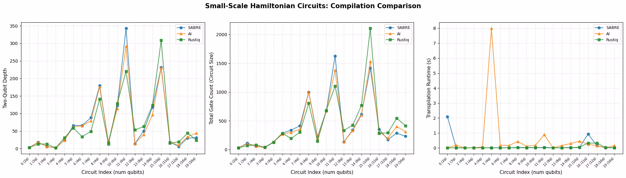
กราฟด้านล่างเปรียบเทียบสามวิธีในแต่ละเมตริกบน circuits แต่ละตัว Circuits จัดเรียงตามจำนวน qubit และแสดงชื่อด้วยดัชนีบนแกน x เนื่องจาก circuits หลายตัวอาจมีจำนวน qubits เท่ากัน
def plot_transpilation_comparison(results, title_prefix):
    """
    Create a three-panel figure comparing compilation methods on
    two-qubit depth, circuit size, and runtime.

    Circuits are sorted by qubit count and plotted by circuit index.
    """
    methods = _method_order(results)
    palette = {"SABRE": "#1f77b4", "AI": "#ff7f0e", "Rustiq": "#2ca02c"}
    markers = {"SABRE": "o", "AI": "^", "Rustiq": "s"}

    # Order circuits by qubit count (then index) and map to plot positions
    ref = sorted(
        [r for r in results if r["method"] == methods[0]],
        key=lambda r: (r["num_qubits"], r["qc_index"]),
    )
    pos_map = {r["qc_index"]: pos for pos, r in enumerate(ref)}
    tick_positions = [pos_map[r["qc_index"]] for r in ref]
    tick_labels = [
        f"{pos_map[r['qc_index']]} ({r['num_qubits']}q)" for r in ref
    ]

    metrics = [
        ("two_qubit_depth", "Two-Qubit Depth"),
        ("size", "Total Gate Count (Circuit Size)"),
        ("runtime", "Transpilation Runtime (s)"),
    ]

    fig, axes = plt.subplots(1, 3, figsize=(20, 5.5))
    fig.suptitle(title_prefix, fontsize=15, fontweight="bold", y=1.02)

    for ax, (metric, ylabel) in zip(axes, metrics):
        for method in methods:
            subset = sorted(
                [r for r in results if r["method"] == method],
                key=lambda r: pos_map[r["qc_index"]],
            )
            ax.plot(
                [pos_map[r["qc_index"]] for r in subset],
                [r[metric] for r in subset],
                marker=markers.get(method, "o"),
                label=method,
                color=palette.get(method, None),
                linewidth=1.5,
                markersize=6,
                alpha=0.85,
            )
        ax.set_xlabel("Circuit Index (num qubits)", fontsize=11)
        ax.set_ylabel(ylabel, fontsize=11)
        ax.legend(frameon=True, fontsize=9)
        ax.grid(True, linestyle="--", alpha=0.4)
        step = max(1, len(tick_positions) // 15)
        ax.set_xticks(tick_positions[::step])
        ax.set_xticklabels(
            [tick_labels[i] for i in range(0, len(tick_labels), step)],
            fontsize=7,
            rotation=45,
            ha="right",
        )

    plt.tight_layout()
    plt.show()
def plot_pct_improvement_vs_sabre(results, title_prefix):
    """
    Plot the per-circuit percent improvement of each non-SABRE method
    relative to SABRE, for each metric. A positive value means the
    method improved on SABRE; negative means SABRE was better.
    """
    metrics = [
        ("two_qubit_depth", "2Q Depth"),
        ("size", "Gate Count"),
        ("runtime", "Runtime"),
    ]
    palette = {"AI": "#ff7f0e", "Rustiq": "#2ca02c"}
    markers = {"AI": "^", "Rustiq": "s"}

    methods = _method_order(results)
    sabre = sorted(
        [r for r in results if r["method"] == "SABRE"],
        key=lambda r: (r["num_qubits"], r["qc_index"]),
    )
    other_methods = [m for m in methods if m != "SABRE"]

    tick_positions = list(range(len(sabre)))
    tick_labels = [
        f"{i} ({sabre[i]['num_qubits']}q)" for i in range(len(sabre))
    ]

    fig, axes = plt.subplots(1, 3, figsize=(20, 5.5))
    fig.suptitle(
        f"{title_prefix}: % Improvement over SABRE",
        fontsize=15,
        fontweight="bold",
        y=1.02,
    )

    for ax, (metric, label) in zip(axes, metrics):
        ax.axhline(0, color="#1f77b4", linewidth=2, label="SABRE (baseline)")
        for method in other_methods:
            data = sorted(
                [r for r in results if r["method"] == method],
                key=lambda r: (r["num_qubits"], r["qc_index"]),
            )
            pct = [
                (sabre[i][metric] - data[i][metric]) / sabre[i][metric] * 100
                for i in range(len(sabre))
            ]
            ax.plot(
                tick_positions,
                pct,
                marker=markers.get(method, "o"),
                label=method,
                color=palette.get(method, None),
                linewidth=1.5,
                markersize=6,
                alpha=0.85,
            )
        ax.set_xlabel("Circuit Index (num qubits)", fontsize=11)
        ax.set_ylabel(f"% Improvement ({label})", fontsize=11)
        ax.legend(frameon=True, fontsize=9)
        ax.grid(True, linestyle="--", alpha=0.4)
        step = max(1, len(tick_positions) // 15)
        ax.set_xticks(tick_positions[::step])
        ax.set_xticklabels(
            [tick_labels[i] for i in range(0, len(tick_labels), step)],
            fontsize=7,
            rotation=45,
            ha="right",
        )
        ylims = ax.get_ylim()
        ax.axhspan(0, max(ylims[1], 1), alpha=0.04, color="green")
        ax.axhspan(min(ylims[0], -1), 0, alpha=0.04, color="red")

    plt.tight_layout()
    plt.show()
plot_transpilation_comparison(
    results_small,
    "Small-Scale Hamiltonian Circuits: Compilation Comparison",
)
plot_pct_improvement_vs_sabre(
    results_small,
    "Small-Scale Hamiltonian Circuits",
)
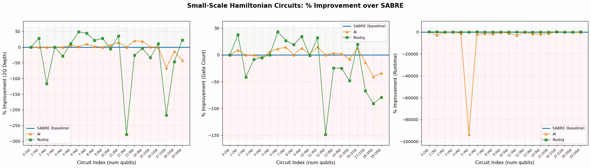
ที่สเกลนี้ pass managers ทั้งสามทำงานได้ดีและผลลัพธ์เฉลี่ยใกล้เคียงกัน ส่วนใหญ่เป็นเพราะ circuits ขนาดเล็กมีพื้นที่จำกัดสำหรับการปรับแต่งเพิ่มเติม ทำให้วิธีต่าง ๆ มักได้ผลลัพธ์ที่คล้ายกัน
ในตัวอย่างนี้ Rustiq ให้ผลลัพธ์ที่แปรปรวนมากที่สุด โดยมี outliers ที่ใหญ่ที่สุดทั้งในด้าน two-qubit depth และ gate count แม้ความแปรปรวนนี้อาจทำให้ตามหลังบ้าง แต่ก็หมายความว่า Rustiq บางครั้งค้นพบ solutions ที่ดีกว่าอีกสองวิธี AI transpiler มีความเสถียรของผลลัพธ์มากกว่าเมื่อเทียบกับ SABRE และ Rustiq โดยติดตามใกล้เคียงกับส่วนใหญ่ของ circuits โดยไม่มี outliers มาก
สำหรับ runtime ทั้ง SABRE และ Rustiq ต่างรวดเร็ว ขณะที่ AI-powered transpiler ช้ากว่าอย่างเห็นได้ชัดบน circuits บางตัว
วิธีที่ทำงานได้ดีที่สุดตามเมตริก
กราฟด้านล่างแสดงความถี่ที่แต่ละวิธีได้รับค่าที่ดีที่สุด (ต่ำที่สุด) สำหรับแต่ละเมตริก เป็นไปได้ที่จะเสมอกัน: สำหรับ circuits ง่าย ๆ หลายวิธีอาจได้ two-qubit depth หรือ gate count ที่ optimal เท่ากัน เมื่อเสมอกัน ทุกวิธีที่เสมอจะได้รับคะแนน ดังนั้นเปอร์เซ็นต์สำหรับเมตริกที่กำหนดอาจรวมกันเกิน 100%
def plot_best_method_bars(results, metrics_list=None):
    """
    Plot a grouped bar chart showing the percentage of circuits
    where each method achieved the best (lowest) value for each metric.

    Ties are counted for all tied methods, so percentages per metric
    can sum to more than 100%.
    """
    if metrics_list is None:
        metrics_list = ["two_qubit_depth", "size", "runtime"]

    labels = {
        "two_qubit_depth": "2Q Depth",
        "size": "Gate Count",
        "runtime": "Runtime",
    }
    methods = _method_order(results)
    palette = {"SABRE": "#1f77b4", "AI": "#ff7f0e", "Rustiq": "#2ca02c"}

    by_index = {}
    for r in results:
        by_index.setdefault(r["qc_index"], []).append(r)
    n_circuits = len(by_index)

    win_data = {m: [] for m in methods}
    tie_counts = []
    metric_labels = []

    for metric in metrics_list:
        metric_labels.append(
            labels.get(metric, metric.replace("_", " ").title())
        )
        counts = Counter()
        ties = 0
        for group in by_index.values():
            min_val = min(r[metric] for r in group)
            best = [r["method"] for r in group if r[metric] == min_val]
            if len(best) > 1:
                ties += 1
            counts.update(best)
        tie_counts.append(ties)
        for m in methods:
            win_data[m].append(counts.get(m, 0) / n_circuits * 100)

    x = np.arange(len(metric_labels))
    width = 0.22
    fig, ax = plt.subplots(figsize=(8, 5))

    for i, method in enumerate(methods):
        bars = ax.bar(
            x + i * width,
            win_data[method],
            width,
            label=method,
            color=palette.get(method, None),
            edgecolor="black",
            linewidth=0.5,
        )
        for bar in bars:
            height = bar.get_height()
            if height > 0:
                ax.text(
                    bar.get_x() + bar.get_width() / 2,
                    height + 1.5,
                    f"{height:.0f}%",
                    ha="center",
                    va="bottom",
                    fontsize=9,
                )

    # Annotate tie counts below each metric label
    for j, ties in enumerate(tie_counts):
        if ties > 0:
            ax.text(
                x[j] + width,
                -8,
                f"({ties} tie{'s' if ties != 1 else ''})",
                ha="center",
                va="top",
                fontsize=8,
                color="gray",
            )

    ax.set_xticks(x + width)
    ax.set_xticklabels(metric_labels, fontsize=11)
    ax.set_ylabel("Circuits with best value (%)", fontsize=11)
    ax.set_title(
        "Best-Performing Method by Metric (ties counted for all tied methods)",
        fontsize=12,
        fontweight="bold",
    )
    ax.legend(frameon=True, fontsize=10)
    ax.set_ylim(-12, 120)
    ax.yaxis.set_major_formatter(ticker.PercentFormatter())
    ax.grid(axis="y", linestyle="--", alpha=0.4)

    plt.tight_layout()
    plt.show()
plot_best_method_bars(results_small)

ในตัวอย่างนี้ สามวิธีทำงานได้ใกล้เคียงกันมากบน circuits ขนาดเล็ก สำหรับ two-qubit depth และ gate count สัดส่วน circuits ที่แต่ละวิธีได้ดีที่สุดใกล้เคียงกัน (ประมาณ 35–55%) และ circuits จำนวนมากเสมอกัน เนื่องจาก circuits ง่าย ๆ มักมี solution ที่ optimal อย่างเดียวที่หลายวิธีค้นพบ ความแตกต่างที่ชัดเจนที่สุดคือ runtime: SABRE และ Rustiq ต่างเร็วที่สุดในประมาณครึ่งหนึ่งของ circuits ขณะที่ AI-powered transpiler แทบไม่เคยเร็วที่สุด เมื่อพิจารณาทั้งสามเมตริกรวมกัน Rustiq มีความได้เปรียบเล็กน้อยโดยรวม เป็นวิธีที่ชนะบ่อยที่สุดใน two-qubit depth และยังคงแข่งขันได้ใน gate count และ runtime
ขั้นตอนที่ 3: รันโดยใช้ Qiskit primitives
เพื่อประเมินว่าคุณภาพ transpilation ส่งผลต่อการรันภายใต้ noise อย่างไร เราใช้เทคนิค mirror circuit สำหรับแต่ละ transpiled circuit เราเพิ่ม inverse เข้าไปเพื่อให้ circuit รวม เป็น identity ในทางทฤษฎี เริ่มต้นจาก state การรันที่สมบูรณ์แบบ (ไม่มี noise) จะคืน all-zeros bitstring ด้วยความน่าจะเป็น 1
ในทางปฏิบัติ ข้อผิดพลาด gate สะสมตลอด circuit ดังนั้นความน่าจะเป็นในการกู้คืน จึงลดลง วิธีการคอมไพล์ที่ผลิต circuit ที่ตื้นกว่าและมี gates น้อยกว่าจะสะสม noise น้อยกว่า
วิธี mirror circuit นั้นเรียบง่ายน่าดึงดูดและขยายไปยัง circuit ขนาดใดก็ได้ เนื่องจาก output ที่คาดหวังคือ เสมอ และไม่ต้องการการจำลอง classical ของ ideal state อย่างไรก็ตาม ควรระวังข้อจำกัดต่อไปนี้: mirror circuit เป็นตัวแทนของ circuit จริง (ไม่ใช่ circuit เอง) มันเพิ่ม gate count เป็นสองเท่า (ซึ่งขยายผลของ noise) และอาจประเมินข้อผิดพลาดบางอย่างต่ำเกินไปเมื่อ noise ยกเลิกกันอย่างสมมาตรข้ามขอบเขต mirror
เราเลือก circuit index 6 จากชุดขนาดเล็กและรัน mirror circuits บน Aer simulator ที่มี depolarizing noise model แบบง่าย
# Select circuit index 6 from the small-scale transpiled circuits
test_idx = 6
test_circuit = qc_small[test_idx]
print(f"Test circuit: {test_circuit.name}, {test_circuit.num_qubits} qubits")

# Get the transpiled versions
tqc_methods_small = {
    "SABRE": tqc_sabre_small[test_idx],
    "AI": tqc_ai_small[test_idx],
    "Rustiq": tqc_rustiq_small[test_idx],
}

# Show transpilation metrics for this circuit
print(f"\nTranspilation metrics for circuit index {test_idx}:")
for method, tqc in tqc_methods_small.items():
    depth_2q = tqc.depth(lambda x: x.operation.num_qubits == 2)
    size = tqc.size()
    print(f"  {method:8s}  2Q depth={depth_2q:5d}  size={size:6d}")
Test circuit: all-vib-fccf, 4 qubits
Transpilation metrics for circuit index 6:
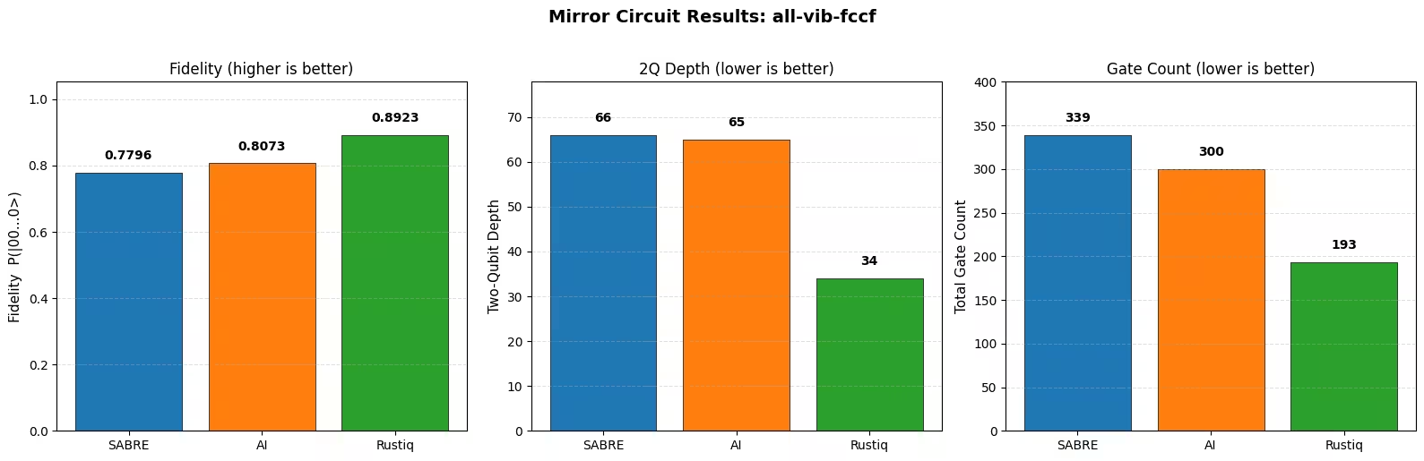
SABRE 2Q depth= 66 size= 339
AI 2Q depth= 65 size= 300
Rustiq 2Q depth= 34 size= 193
สร้าง mirror circuits (เพิ่ม ) แมปไปยังดัชนี qubit ต่อเนื่องเพื่อให้ simulator จัดการเฉพาะ qubits ที่ใช้งาน และรันบน Aer simulator ที่มี noise
def remap_to_contiguous(tqc):
    """Remap a transpiled circuit to use contiguous qubit indices.

    Transpiled circuits target specific physical qubits (e.g., qubit 45, 67)
    on a large backend. This remaps them to 0, 1, 2, ... so Aer only
    simulates the active qubits.
    """
    active = sorted(
        {tqc.find_bit(q).index for inst in tqc.data for q in inst.qubits}
    )
    qubit_map = {old: new for new, old in enumerate(active)}
    new_qc = QuantumCircuit(len(active))
    for inst in tqc.data:
        old_indices = [tqc.find_bit(q).index for q in inst.qubits]
        new_qc.append(inst.operation, [qubit_map[i] for i in old_indices])
    return new_qc

def build_mirror_circuit(tqc):
    """Build a mirror circuit: U followed by U-dagger, with measurements.

    The combined circuit U-dagger @ U should be the identity, so measuring
    all zeros indicates a noise-free execution.
    """
    tqc_compact = remap_to_contiguous(tqc)
    mirror = tqc_compact.compose(tqc_compact.inverse())
    mirror.measure_all()
    return mirror

# Build a simple depolarizing noise model
noise_model = NoiseModel()
noise_model.add_all_qubit_quantum_error(
    depolarizing_error(0.001, 1),
    ["sx", "x", "rz"],  # ~0.1% per 1Q gate
)
noise_model.add_all_qubit_quantum_error(
    depolarizing_error(0.01, 2),
    ["cx", "ecr"],  # ~1% per 2Q gate
)

aer_sim = AerSimulator(noise_model=noise_model)

shots = 10000
fidelities = {}

for method, tqc in tqc_methods_small.items():
    mirror = build_mirror_circuit(tqc)

    sampler = SamplerV2(mode=aer_sim)
    job = sampler.run([mirror], shots=shots)
    result = job.result()
    counts = result[0].data.meas.get_counts()

    # Fidelity = fraction of all-zeros (error-free) outcomes
    n_qubits = mirror.num_qubits - mirror.num_clbits  # active qubits
    all_zeros = "0" * mirror.num_qubits
    fidelity = counts.get(all_zeros, 0) / shots
    fidelities[method] = fidelity
    print(
        f"{method:8s}  P(|00...0>) = {fidelity:.4f}  ({counts.get(all_zeros, 0)}/{shots})"
    )
SABRE     P(|00...0>) = 0.7796  (7796/10000)
AI        P(|00...0>) = 0.8073  (8073/10000)
Rustiq    P(|00...0>) = 0.8923  (8923/10000)
def plot_mirror_results(tqc_methods, fidelities, circuit_name):
    """
    Plot a three-panel comparison: fidelity, 2Q depth,
    and gate count for each compilation method.
    """
    methods = list(tqc_methods.keys())
    palette = {"SABRE": "#1f77b4", "AI": "#ff7f0e", "Rustiq": "#2ca02c"}
    colors = [palette.get(m, "gray") for m in methods]

    fidelity_vals = [fidelities[m] for m in methods]
    depth_vals = [
        tqc_methods[m].depth(lambda x: x.operation.num_qubits == 2)
        for m in methods
    ]
    size_vals = [tqc_methods[m].size() for m in methods]

    fig, axes = plt.subplots(1, 3, figsize=(16, 5))
    fig.suptitle(
        f"Mirror Circuit Results: {circuit_name}",
        fontsize=14,
        fontweight="bold",
        y=1.02,
    )

    def _annotate_bars(ax, bars, values, fmt="{}"):
        ymax = ax.get_ylim()[1]
        for bar, val in zip(bars, values):
            label = fmt.format(val)
            y = val + ymax * 0.03
            ax.text(
                bar.get_x() + bar.get_width() / 2,
                y,
                label,
                ha="center",
                va="bottom",
                fontsize=10,
                fontweight="bold",
            )

    # Panel 1: Survival Probability
    bars = axes[0].bar(
        methods, fidelity_vals, color=colors, edgecolor="black", linewidth=0.5
    )
    axes[0].set_ylabel("Fidelity  P(|00...0>)", fontsize=11)
    axes[0].set_title("Fidelity (higher is better)", fontsize=12)
    axes[0].set_ylim(
        0, max(fidelity_vals) * 1.18 if max(fidelity_vals) > 0 else 1.0
    )
    axes[0].grid(axis="y", linestyle="--", alpha=0.4)
    _annotate_bars(axes[0], bars, fidelity_vals, fmt="{:.4f}")

    # Panel 2: Two-Qubit Depth
    bars = axes[1].bar(
        methods, depth_vals, color=colors, edgecolor="black", linewidth=0.5
    )
    axes[1].set_ylabel("Two-Qubit Depth", fontsize=11)
    axes[1].set_title("2Q Depth (lower is better)", fontsize=12)
    axes[1].set_ylim(0, max(depth_vals) * 1.18)
    axes[1].grid(axis="y", linestyle="--", alpha=0.4)
    _annotate_bars(axes[1], bars, depth_vals)

    # Panel 3: Gate Count
    bars = axes[2].bar(
        methods, size_vals, color=colors, edgecolor="black", linewidth=0.5
    )
    axes[2].set_ylabel("Total Gate Count", fontsize=11)
    axes[2].set_title("Gate Count (lower is better)", fontsize=12)
    axes[2].set_ylim(0, max(size_vals) * 1.18)
    axes[2].grid(axis="y", linestyle="--", alpha=0.4)
    _annotate_bars(axes[2], bars, size_vals)

    plt.tight_layout()
    plt.show()

plot_mirror_results(tqc_methods_small, fidelities, test_circuit.name)
ข้อสังเกต
วิธีที่มี two-qubit depth ต่ำสุดและมี gates น้อยที่สุดได้ fidelity สูงสุด สอดคล้องกับความคาดหวังว่า circuits ที่สั้นกว่าจะสะสม noise น้อยกว่า แม้ความแตกต่างเพียงเล็กน้อยใน depth และ gate count ก็แปลเป็นความแตกต่างที่วัดได้ใน fidelity ภายใต้ depolarizing noise model
โปรดจำไว้ว่าผลลัพธ์เหล่านี้สำหรับ circuit เดียว การจัดอันดับสัมพัทธ์ของวิธีต่าง ๆ อาจเปลี่ยนแปลงไปตาม circuit ขึ้นอยู่กับโครงสร้าง Hamiltonian
ตัวอย่างฮาร์ดแวร์ขนาดใหญ่
ในส่วนนี้ เราเปรียบเทียบวิธีการคอมไพล์ทั้งสามแบบเดิมบน Hamiltonian circuits ที่มี 20 qubits ขึ้นไป Circuit เหล่านี้เป็นตัวแทนของภาระงาน Hamiltonian simulation ที่ใช้งานจริงมากกว่า และทดสอบการขยายของแต่ละวิธีในด้านคุณภาพ circuit และเวลาการคอมไพล์
ขั้นตอนที่ 1-4 รวมกัน
workflow ตามโครงสร้างเดียวกับตัวอย่างขนาดเล็ก เราทำ transpile circuits ขนาดใหญ่ทั้งหมดด้วยแต่ละวิธี เก็บเมตริก และส่ง mirror circuit ไปยังฮาร์ดแวร์ quantum จริง
results_large = []

tqc_sabre_large = capture_transpilation_metrics(
    results_large, pm_sabre, qc_large, "SABRE"
)
tqc_ai_large = capture_transpilation_metrics(
    results_large, pm_ai, qc_large, "AI"
)
tqc_rustiq_large = capture_transpilation_metrics(
    results_large, pm_rustiq, qc_large, "Rustiq"
)
[SABRE] Circuit 0 (all-vib-hc3h2cn): 2Q depth=2, size=258, time=0.16s
[SABRE] Circuit 1 (ham-graph-gnp_k-5): 2Q depth=345, size=4036, time=0.08s
[SABRE] Circuit 2 (TSP_Ncity-5): 2Q depth=187, size=2045, time=0.04s
[SABRE] Circuit 3 (tfim): 2Q depth=100, size=489, time=0.21s
[SABRE] Circuit 4 (all-vib-h2co): 2Q depth=30, size=570, time=0.18s
[SABRE] Circuit 5 (uuf100-ham): 2Q depth=414, size=4779, time=0.09s
[SABRE] Circuit 6 (uuf100-ham): 2Q depth=523, size=5667, time=0.11s
[SABRE] Circuit 7 (graph-gnp_k-4): 2Q depth=3028, size=24885, time=0.39s
[SABRE] Circuit 8 (uf100-ham): 2Q depth=700, size=8271, time=0.15s
[SABRE] Circuit 9 (uf100-ham): 2Q depth=698, size=8957, time=0.15s
[SABRE] Circuit 10 (TSP_Ncity-7): 2Q depth=432, size=6353, time=0.12s
[SABRE] Circuit 11 (all-vib-cyclo_propene): 2Q depth=30, size=1144, time=0.20s
[SABRE] Circuit 12 (TSP_Ncity-8): 2Q depth=704, size=10287, time=0.18s
[SABRE] Circuit 13 (uf100-ham): 2Q depth=2454, size=30195, time=0.46s
[SABRE] Circuit 14 (tfim): 2Q depth=245, size=3670, time=0.08s
[SABRE] Circuit 15 (flat100-ham): 2Q depth=154, size=3836, time=0.12s
[SABRE] Circuit 16 (graph-regular_reg-4): 2Q depth=863, size=14063, time=0.22s
[SABRE] Circuit 17 (tfim): 2Q depth=581, size=8810, time=0.15s
[SABRE] Circuit 18 (FH_D-1): 2Q depth=1704, size=9528, time=0.35s
[SABRE] Circuit 19 (TSP_Ncity-10): 2Q depth=1091, size=22041, time=0.38s
[SABRE] Circuit 20 (TSP_Ncity-10): 2Q depth=1091, size=22005, time=0.38s
[SABRE] Circuit 21 (ham-unary-color02-queen13_13_k-4): 2Q depth=224, size=8321, time=0.17s
[AI] Circuit 0 (all-vib-hc3h2cn): 2Q depth=2, size=258, time=0.17s
[AI] Circuit 1 (ham-graph-gnp_k-5): 2Q depth=323, size=4418, time=3.13s
[AI] Circuit 2 (TSP_Ncity-5): 2Q depth=161, size=2229, time=1.47s
[AI] Circuit 3 (tfim): 2Q depth=20, size=402, time=0.34s
[AI] Circuit 4 (all-vib-h2co): 2Q depth=38, size=661, time=0.19s
[AI] Circuit 5 (uuf100-ham): 2Q depth=391, size=5130, time=3.27s
[AI] Circuit 6 (uuf100-ham): 2Q depth=463, size=6095, time=4.23s
[AI] Circuit 7 (graph-gnp_k-4): 2Q depth=3207, size=25641, time=15.15s
[AI] Circuit 8 (uf100-ham): 2Q depth=637, size=8267, time=5.87s
[AI] Circuit 9 (uf100-ham): 2Q depth=632, size=9330, time=7.29s
[AI] Circuit 10 (TSP_Ncity-7): 2Q depth=452, size=7418, time=6.02s
[AI] Circuit 11 (all-vib-cyclo_propene): 2Q depth=38, size=1323, time=0.27s
[AI] Circuit 12 (TSP_Ncity-8): 2Q depth=609, size=11131, time=10.07s
[AI] Circuit 13 (uf100-ham): 2Q depth=2251, size=31128, time=38.77s
[AI] Circuit 14 (tfim): 2Q depth=165, size=3460, time=1.64s
[AI] Circuit 15 (flat100-ham): 2Q depth=91, size=3497, time=2.49s
[AI] Circuit 16 (graph-regular_reg-4): 2Q depth=664, size=15256, time=12.35s
[AI] Circuit 17 (tfim): 2Q depth=583, size=9157, time=6.28s
[AI] Circuit 18 (FH_D-1): 2Q depth=1193, size=7754, time=4.54s
[AI] Circuit 19 (TSP_Ncity-10): 2Q depth=1134, size=22577, time=25.64s
[AI] Circuit 20 (TSP_Ncity-10): 2Q depth=1172, size=23851, time=28.97s
[AI] Circuit 21 (ham-unary-color02-queen13_13_k-4): 2Q depth=219, size=8600, time=8.85s
[Rustiq] Circuit 0 (all-vib-hc3h2cn): 2Q depth=2, size=257, time=0.16s
[Rustiq] Circuit 1 (ham-graph-gnp_k-5): 2Q depth=640, size=5831, time=0.13s
[Rustiq] Circuit 2 (TSP_Ncity-5): 2Q depth=408, size=3985, time=0.08s
[Rustiq] Circuit 3 (tfim): 2Q depth=31, size=688, time=0.07s
[Rustiq] Circuit 4 (all-vib-h2co): 2Q depth=65, size=1058, time=2.91s
[Rustiq] Circuit 5 (uuf100-ham): 2Q depth=633, size=6757, time=0.14s
[Rustiq] Circuit 6 (uuf100-ham): 2Q depth=795, size=8495, time=0.17s
[Rustiq] Circuit 7 (graph-gnp_k-4): 2Q depth=13768, size=139793, time=2.92s
[Rustiq] Circuit 8 (uf100-ham): 2Q depth=1099, size=11878, time=0.25s
[Rustiq] Circuit 9 (uf100-ham): 2Q depth=911, size=11111, time=0.22s
[Rustiq] Circuit 10 (TSP_Ncity-7): 2Q depth=1183, size=13197, time=0.27s
[Rustiq] Circuit 11 (all-vib-cyclo_propene): 2Q depth=67, size=2491, time=13.56s
[Rustiq] Circuit 12 (TSP_Ncity-8): 2Q depth=1615, size=21358, time=0.48s
[Rustiq] Circuit 13 (uf100-ham): 2Q depth=2920, size=40465, time=0.91s
[Rustiq] Circuit 14 (tfim): 2Q depth=489, size=6552, time=0.15s
[Rustiq] Circuit 15 (flat100-ham): 2Q depth=378, size=5906, time=0.14s
[Rustiq] Circuit 16 (graph-regular_reg-4): 2Q depth=12163, size=168679, time=2.94s
[Rustiq] Circuit 17 (tfim): 2Q depth=1208, size=17042, time=0.36s
[Rustiq] Circuit 18 (FH_D-1): 2Q depth=1061, size=24000, time=0.47s
[Rustiq] Circuit 19 (TSP_Ncity-10): 2Q depth=2565, size=41340, time=1.38s
[Rustiq] Circuit 20 (TSP_Ncity-10): 2Q depth=2565, size=41275, time=1.38s
[Rustiq] Circuit 21 (ham-unary-color02-queen13_13_k-4): 2Q depth=808, size=17548, time=0.42s
print_summary_table(results_large)
Mean +/- std per compilation method
Method                2Q Depth              Gate Count             Runtime (s)
------------------------------------------------------------------------------
SABRE          709.1 +/- 783.8     9,100.5 +/- 8,493.1             0.2 +/- 0.1
AI             656.6 +/- 777.5     9,435.6 +/- 8,853.0            8.5 +/- 10.2
Rustiq     2,062.5 +/- 3,631.1   26,804.8 +/- 43,403.1             1.3 +/- 2.9

Mean % improvement vs SABRE (positive = better than SABRE)
Method                2Q Depth              Gate Count             Runtime (s)
------------------------------------------------------------------------------
AI             +9.6% +/- 22.8%          -3.4% +/- 9.4%    -3620.0% +/- 2405.5%
Rustiq      -154.5% +/- 273.9%      -137.1% +/- 233.2%     -527.0% +/- 1405.5%
print_per_circuit_comparison(results_large, num_rows=8)
2Q Depth (first 8 circuits by qubit count); * = best
Idx  Circuit            Q    SABRE       AI   Rustiq
----------------------------------------------------
  0  all-vib-hc3h2cn   24       2*       2*       2*
  1  ham-graph-gnp_k-  24      345     323*      640
  2  TSP_Ncity-5       25      187     161*      408
  3  tfim              26      100      20*       31
  4  all-vib-h2co      32      30*       38       65
  5  uuf100-ham        40      414     391*      633
  6  uuf100-ham        40      523     463*      795
  7  graph-gnp_k-4     40    3028*     3207    13768

Gate Count (first 8 circuits by qubit count); * = best
Idx  Circuit            Q    SABRE       AI   Rustiq
----------------------------------------------------
  0  all-vib-hc3h2cn   24      258      258     257*
  1  ham-graph-gnp_k-  24    4036*     4418     5831
  2  TSP_Ncity-5       25    2045*     2229     3985
  3  tfim              26      489     402*      688
  4  all-vib-h2co      32     570*      661     1058
  5  uuf100-ham        40    4779*     5130     6757
  6  uuf100-ham        40    5667*     6095     8495
  7  graph-gnp_k-4     40   24885*    25641   139793

Runtime (s) (first 8 circuits by qubit count); * = best
Idx  Circuit            Q    SABRE       AI   Rustiq
----------------------------------------------------
  0  all-vib-hc3h2cn   24     0.16     0.17    0.16*
  1  ham-graph-gnp_k-  24    0.08*     3.13     0.13
  2  TSP_Ncity-5       25    0.04*     1.47     0.08
  3  tfim              26     0.21     0.34    0.07*
  4  all-vib-h2co      32    0.18*     0.19     2.91
  5  uuf100-ham        40    0.09*     3.27     0.14
  6  uuf100-ham        40    0.11*     4.23     0.17
  7  graph-gnp_k-4     40    0.39*    15.15     2.92
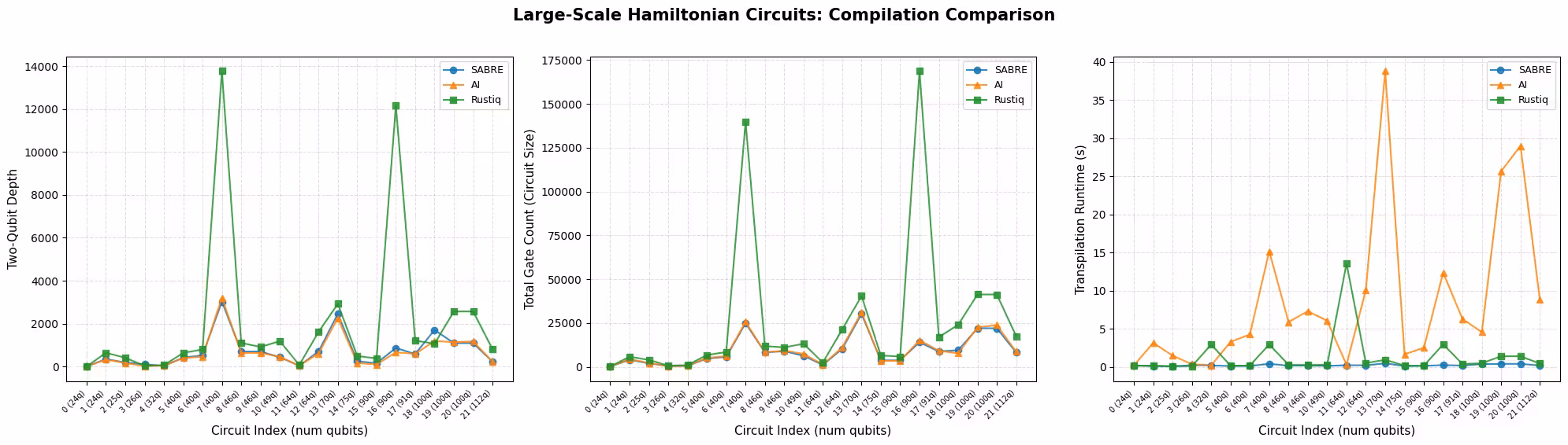
plot_transpilation_comparison(
    results_large,
    "Large-Scale Hamiltonian Circuits: Compilation Comparison",
)
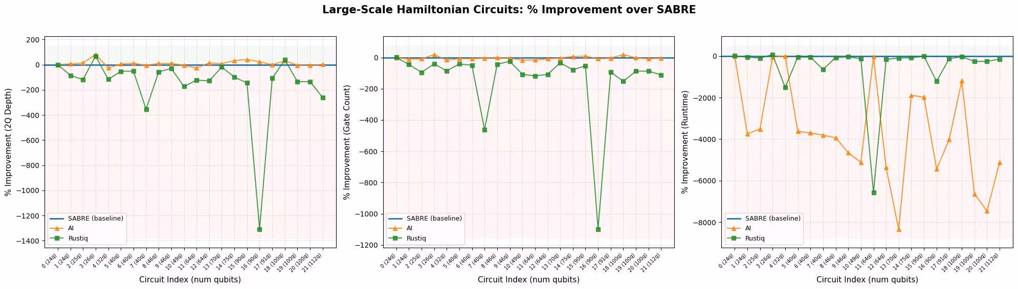
plot_pct_improvement_vs_sabre(
    results_large,
    "Large-Scale Hamiltonian Circuits",
)
plot_best_method_bars(results_large)

# Select circuit index 3 from the large-scale transpiled circuits
test_idx_large = 3
test_circuit_large = qc_large[test_idx_large]
print(
    f"Test circuit: {test_circuit_large.name}, {test_circuit_large.num_qubits} qubits"
)

tqc_methods_large = {
    "SABRE": tqc_sabre_large[test_idx_large],
    "AI": tqc_ai_large[test_idx_large],
    "Rustiq": tqc_rustiq_large[test_idx_large],
}

print(f"\nTranspilation metrics for circuit index {test_idx_large}:")
for method, tqc in tqc_methods_large.items():
    depth_2q = tqc.depth(lambda x: x.operation.num_qubits == 2)
    size = tqc.size()
    print(f"  {method:8s}  2Q depth={depth_2q:5d}  size={size:6d}")
Test circuit: tfim, 26 qubits

Transpilation metrics for circuit index 3:
  SABRE     2Q depth=  100  size=   489
  AI        2Q depth=   20  size=   402
  Rustiq    2Q depth=   31  size=   688
pm_mirror = generate_preset_pass_manager(
    optimization_level=0, backend=backend
)

for method, tqc in tqc_methods_large.items():
    # print the count ops for each circuit
    mirror = tqc.copy()
    mirror.compose(tqc.inverse(), inplace=True)
    mirror.measure_all()
    mirror = pm_mirror.run(mirror)
    print(f"\n{method} transpiled circuit:")
    print(tqc.count_ops())
    print(f"{method} mirror circuit count ops:")
    print(mirror.count_ops())
SABRE transpiled circuit:
OrderedDict({'sx': 211, 'rz': 163, 'cz': 104, 'x': 11})
SABRE mirror circuit count ops:
OrderedDict({'rz': 1170, 'sx': 422, 'cz': 208, 'measure': 156, 'x': 22, 'barrier': 1})

AI transpiled circuit:
OrderedDict({'sx': 165, 'rz': 162, 'cz': 68, 'x': 7})
AI mirror circuit count ops:
OrderedDict({'rz': 984, 'sx': 330, 'measure': 156, 'cz': 136, 'x': 14, 'barrier': 1})

Rustiq transpiled circuit:
OrderedDict({'sx': 316, 'rz': 225, 'cz': 140, 'x': 7})
Rustiq mirror circuit count ops:
OrderedDict({'rz': 1714, 'sx': 632, 'cz': 280, 'measure': 156, 'x': 14, 'barrier': 1})
# Build mirror circuits and submit to real hardware
# The inverse may introduce gates (e.g., sxdg) not in the backend's
# basis gate set, so we re-transpile the mirror circuit.
pm_mirror = generate_preset_pass_manager(
    optimization_level=0, backend=backend
)

shots_hw = 10000
hw_jobs = {}

for method, tqc in tqc_methods_large.items():
    mirror = tqc.copy()
    mirror.compose(tqc.inverse(), inplace=True)
    mirror.measure_all()

    # Re-transpile at opt level 0 to decompose into basis gates
    # without changing the layout or routing
    mirror = pm_mirror.run(mirror)

    sampler = SamplerV2(mode=backend)
    sampler.options.environment.job_tags = ["TUT_CMHSC"]
    job = sampler.run([mirror], shots=shots_hw)
    hw_jobs[method] = job
    print(f"{method}: submitted job {job.job_id()}")
SABRE: submitted job d8gvgq66983c73dqe5og
AI: submitted job d8gvgqe6983c73dqe5pg
Rustiq: submitted job d8gvgqm6983c73dqe5q0
# Retrieve results and compute fidelities
fidelities_large = {}

for method, job in hw_jobs.items():
    result = job.result()
    counts = result[0].data.meas.get_counts()

    n_qubits = backend.num_qubits
    all_zeros = "0" * n_qubits
    fidelity = counts.get(all_zeros, 0) / shots_hw
    fidelities_large[method] = fidelity
    print(
        f"{method:8s}  P(|00...0>) = {fidelity:.4f}  ({counts.get(all_zeros, 0)}/{shots_hw})"
    )
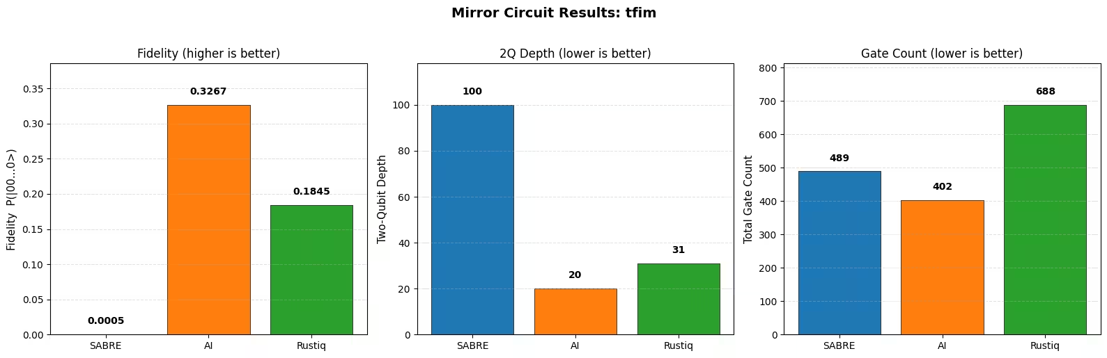
SABRE     P(|00...0>) = 0.0005  (5/10000)
AI        P(|00...0>) = 0.3267  (3267/10000)
Rustiq    P(|00...0>) = 0.1845  (1845/10000)
plot_mirror_results(
    tqc_methods_large, fidelities_large, test_circuit_large.name
)
การวิเคราะห์ผลการคอมไพล์
การเปรียบเทียบข้างต้นเปรียบเทียบ SABRE, AI-powered transpiler และ Rustiq บน Hamiltonian simulation circuits จากชุด Hamlib ทั้งในระดับขนาดเล็กและขนาดใหญ่
Two-qubit depth และ gate count
ที่สเกลขนาดใหญ่ SABRE และ AI-powered transpiler เป็นสองวิธีที่ทำงานได้ดีที่สุด โดยแต่ละวิธีนำในเมตริกที่แตกต่างกัน ดังที่กราฟ วิธีที่ทำงานได้ดีที่สุดตามเมตริก แสดงให้เห็น SABRE ผลิต gate count ต่ำสุดบน circuits ส่วนใหญ่และเป็นวิธีที่เร็วที่สุดบนเกือบทุก circuit สอดคล้องกับ heuristic ที่ออกแบบมาเพื่อลด SWAP gates ที่แทรกเข้ามา และการปรับปรุงล่าสุดใน layout และ routing AI-powered transpiler ผลิต two-qubit depth ต่ำสุดบน circuits ส่วนใหญ่ สอดคล้องกับส่วนของ objective ใน reinforcement learning ที่มุ่งเป้าที่ circuit depth ตารางสรุปแสดงการแบ่งเช่นเดียวกัน: SABRE มี gate count เฉลี่ยต่ำกว่า ขณะที่ AI transpiler มี two-qubit depth เฉลี่ยต่ำกว่า ทั้งสองวิธีมีความสม่ำเสมอและน่าเชื่อถือข้าม circuits ทุกช่วง
Rustiq ซึ่งออกแบบมาเป็นพิเศษสำหรับการสังเคราะห์ PauliEvolutionGate ผลิตผลลัพธ์ที่ดีที่สุดเพียงในสัดส่วนเล็กน้อยของ circuits ขนาดใหญ่ เมตริกเฉลี่ยของมันถูกบิดเบือนอย่างมากจาก outliers จำนวนหนึ่ง ซึ่งมองเห็นได้เป็นยอดสูงใน compilation comparison plot ที่ Rustiq ผลิต depth และ gate count สูงกว่าวิธีอื่นมาก หากไม่มี outliers เหล่านี้ ประสิทธิภาพเฉลี่ยจะใกล้เคียงกับ SABRE และ AI-powered transpiler มากกว่า
ข้อสังเกตสำคัญคือไม่มีวิธีเดียวที่ครอบงำทุก circuit แต่ละวิธีทำงานได้ดีกว่าวิธีอื่นในกรณีเฉพาะ ดังนั้นจึงคุ้มค่าที่จะลองใช้เครื่องมือที่มีอยู่ทั้งหมดและเลือกผลลัพธ์ที่ดีที่สุดสำหรับแต่ละ circuit
Runtime
SABRE เป็นวิธีที่เร็วที่สุดอย่างสม่ำเสมอ Rustiq โดยทั่วไปทำงานด้วยความเร็วใกล้เคียงกัน แต่อาจผลิต outliers ที่การคอมไพล์ใช้เวลานานกว่ามาก สิ่งนี้เห็นได้ชัดเจนเป็นพิเศษในผลลัพธ์ขนาดใหญ่ ที่ circuits บางตัวทำให้ runtime ของ Rustiq พุ่งสูงขึ้น outliers เหล่านี้ส่งผลกระทบอย่างมากต่อ runtime เฉลี่ย ดังนั้น median อาจเป็นสรุปที่เป็นตัวแทนมากกว่าสำหรับ Rustiq AI-powered transpiler เป็นวิธีที่ช้าที่สุดในสามแบบ โดย runtime เพิ่มขึ้นอย่างเห็นได้ชัดบน circuits ที่ใหญ่กว่าและซับซ้อนกว่า
ผลลัพธ์ Mirror circuit
การทดลอง mirror circuit ยืนยันแนวโน้มที่คาดหวัง: วิธีที่ผลิต two-qubit depth ต่ำกว่าและมี gates น้อยกว่าได้ fidelity สูงกว่าภายใต้ noise ซึ่งเป็นจริงทั้งบน noisy simulator (ขนาดเล็ก) และฮาร์ดแวร์จริง (ขนาดใหญ่)
โปรดจำไว้ว่ากราฟ mirror circuit แต่ละอันแสดง circuit เดียว ไม่ใช่ผลรวม ตัวอย่างฮาร์ดแวร์ข้างต้นใช้ circuit tfim 26-qubit หนึ่งตัว ซึ่งเป็นกรณีที่ SABRE ผลิต two-qubit depth สูงกว่า AI-powered transpiler และ Rustiq มาก ดังนั้น fidelity จึงต่ำกว่าอย่างสอดคล้องกัน สิ่งนี้ไม่ได้เป็นตัวแทนของผลลัพธ์ในวงกว้าง: ข้าม circuits ขนาดใหญ่ทั้งหมด two-qubit depth ของ SABRE มักใกล้เคียงกับ AI-powered transpiler และทั้งสองวิธีต่างนำในเมตริกที่แตกต่างกัน (AI-powered transpiler ใน two-qubit depth, SABRE ใน gate count และ runtime) ผลลัพธ์ mirror เดียวทดสอบเวอร์ชันที่เพิ่มเป็นสองเท่าของ circuit หนึ่งตัวมากกว่าภาระงานทั้งหมด ดังนั้นไม่ควรอ่านเป็นคำตัดสินเกี่ยวกับคุณภาพของวิธีโดยรวม
คำแนะนำ
ไม่มีกลยุทธ์ transpilation ที่ดีที่สุดเพียงอย่างเดียวสำหรับทุก circuit การเลือกที่ดีที่สุดขึ้นอยู่กับโครงสร้าง circuit เป้าหมายการปรับแต่ง และงบประมาณเวลาการคอมไพล์ที่มีอยู่:
- SABRE เป็นค่าเริ่มต้นที่แนะนำ รวดเร็วและน่าเชื่อถือ และผลิตผลลัพธ์ที่ดีข้าม circuits หลากหลาย สำหรับการปรับแต่งเพิ่มเติม ผู้ใช้สามารถเพิ่ม layout และ routing trials (ดู บทช่วยสอนการปรับแต่ง SABRE)
- AI-powered transpiler คุ้มค่าที่จะลองเมื่อเวลาการคอมไพล์ไม่ใช่ข้อจำกัด โดยเฉพาะเมื่อการลด two-qubit depth เป็นสิ่งสำคัญ: มันผลิต two-qubit depth ต่ำสุดบน circuits ขนาดใหญ่ส่วนใหญ่ใน benchmark นี้
- Rustiq ออกแบบมาสำหรับ
PauliEvolutionGatecircuits และสามารถค้นพบ solutions ที่มี depth ต่ำและ gate count น้อยมาก โดยเฉพาะบน circuits ขนาดเล็ก บน circuits ขนาดใหญ่บางครั้งอาจผลิตผลลัพธ์ที่ใหญ่กว่ามาก ดังนั้นจึงดีที่สุดเมื่อใช้เป็นหนึ่งในหลายวิธีที่ลองมากกว่าเป็นค่าเริ่มต้น
ในทางปฏิบัติ วิธีที่ดีที่สุดคือรันทุกวิธีที่มีอยู่และเลือกผลลัพธ์ที่ดีที่สุดสำหรับแต่ละ circuit ต้นทุนการคอมไพล์จากการลองหลายวิธีมีน้อยมากเมื่อเทียบกับการปรับปรุงคุณภาพการรันบนฮาร์ดแวร์จริงที่อาจได้รับ
ขั้นตอนต่อไป
หากคุณพบว่าบทช่วยสอนนี้มีประโยชน์ คุณอาจสนใจสิ่งต่อไปนี้:
อ้างอิง
[1] "LightSABRE: A Lightweight and Enhanced SABRE Algorithm". H. Zou, M. Treinish, K. Hartman, A. Ivrii, J. Lishman et al. https://arxiv.org/abs/2409.08368
[2] "Practical and efficient quantum circuit synthesis and transpiling with Reinforcement Learning". D. Kremer, V. Villar, H. Paik, I. Duran, I. Faro, J. Cruz-Benito et al. https://arxiv.org/abs/2405.13196
[3] "Pauli Network Circuit Synthesis with Reinforcement Learning". A. Dubal, D. Kremer, S. Martiel, V. Villar, D. Wang, J. Cruz-Benito et al. https://arxiv.org/abs/2503.14448
[4] "Faster and shorter synthesis of Hamiltonian simulation circuits". T. Goubault de Brugiere, S. Martiel et al. https://arxiv.org/abs/2404.03280