การพัวพันระยะไกลด้วย Dynamic Circuits
ประมาณการใช้งาน: 4 นาที บน Heron r2 processor (หมายเหตุ: นี่เป็นเพียงการประมาณเท่านั้น ระยะเวลาจริงอาจแตกต่างกันได้)
ผลการเรียนรู้
หลังจากเรียนบทเรียนนี้เสร็จสิ้น คุณจะได้เรียนรู้สิ่งต่อไปนี้:
- วิธีนำ long-range CNOT gate ไปใช้งานโดยใช้ dynamic circuits ด้วย mid-circuit measurements (MCMs) และ classical feedforward;
- วิธีนำ Gate ที่เทียบเท่าไปใช้งานโดยใช้แนวทาง unitary SWAP-based;
- วิธีเปรียบเทียบทั้งสองแนวทางโดยวัด gate fidelity เป็นฟังก์ชันของระยะห่างระหว่าง Qubit
สิ่งที่ต้องรู้ก่อน
เราแนะนำให้ผู้ใช้คุ้นเคยกับหัวข้อต่อไปนี้ก่อนเรียนบทเรียนนี้:
- แนวคิดพื้นฐานของการคำนวณควอนตัม ได้แก่ Bell states, entanglement, และ quantum gates;
- ความคุ้นเคยกับ dynamic circuits (mid-circuit measurements และ classical feedforward);
- ความรู้พื้นฐานเกี่ยวกับ Qiskit SDK และ Qiskit Runtime และการเข้าถึง IBM Quantum® account
พื้นหลัง
การสร้างพัวพัน (entanglement) ระยะไกลระหว่าง Qubit ที่อยู่ห่างกันนั้นเป็นเรื่องท้าทายบนอุปกรณ์ที่มีการเชื่อมต่อจำกัด บทเรียนนี้แสดงให้เห็นว่า dynamic circuits สามารถสร้างพัวพันดังกล่าวได้อย่างไร โดยการนำ long-range controlled-X (LRCX) Gate ไปใช้งานผ่านโปรโตคอลที่อาศัยการวัด
ตามแนวทางของ Elisa Bäumer et al. ใน 1 วิธีนี้ใช้การวัดกลาง Circuit และ feedforward เพื่อให้ได้ Gate ความลึกคงที่ไม่ว่า Qubit จะห่างกันแค่ไหน โดยสร้าง Bell pairs ตัวกลาง วัด Qubit หนึ่งตัวจากแต่ละคู่ แล้วนำ Gate ที่กำหนดเงื่อนไขทางคลาสสิกมาใช้เพื่อถ่ายทอดพัวพันข้ามอุปกรณ์ วิธีนี้หลีกเลี่ยงห่วงโซ่ SWAP ยาว ลดทั้งความลึกของ Circuit และการสัมผัสกับข้อผิดพลาดของ two-qubit gate
ใน notebook นี้ เราปรับโปรโตคอลให้เข้ากับฮาร์ดแวร์ IBM Quantum และประเมินประสิทธิภาพเป็นฟังก์ชันของระยะห่างระหว่าง control และ target โดยเปรียบเทียบกับ unitary SWAP-based baseline
ข้อกำหนด
ก่อนเริ่มบทเรียนนี้ ให้ตรวจสอบว่าได้ติดตั้งสิ่งต่อไปนี้แล้ว:
- Qiskit SDK v2.0 หรือใหม่กว่า พร้อมรองรับ visualization
- Qiskit Runtime v0.37 หรือใหม่กว่า (
pip install qiskit-ibm-runtime) - Qiskit Aer v0.17 หรือใหม่กว่า (
pip install qiskit-aer)
การตั้งค่า
# Added by doQumentation — required packages for this notebook
!pip install -q matplotlib numpy qiskit qiskit-aer qiskit-ibm-runtime
from qiskit import QuantumCircuit, QuantumRegister, ClassicalRegister
from qiskit.circuit.classical import expr
from qiskit.transpiler import generate_preset_pass_manager
from qiskit.visualization import plot_circuit_layout
from qiskit_ibm_runtime import (
    QiskitRuntimeService,
    Batch,
    SamplerV2 as Sampler,
)
import matplotlib.pyplot as plt
import numpy as np
ตัวอย่างจำลองขนาดเล็ก
ก่อนรันบนฮาร์ดแวร์ QPU จริง เราตรวจสอบว่าทั้ง dynamic และ unitary circuits ให้ Bell state ในอุดมคติบน simulator ที่ไม่มีสัญญาณรบกวน เราใช้ Qiskit Runtime Sampler กับ AerSimulator เป็น backend mode ที่ระยะห่าง 6
ขั้นตอนที่ 1: แปลงข้อมูลนำเข้าแบบคลาสสิกเป็นปัญหาควอนตัม
ตอนนี้เราจะสร้าง long-range CNOT Gate ระหว่าง Qubit สองตัวที่อยู่ห่างกัน โดยใช้โครงสร้าง dynamic circuit ที่แสดงด้านล่าง (ปรับมาจาก Fig. 1a ใน Ref. 1) แนวคิดหลักคือการใช้ "bus" ของ Qubit สำรอง ที่เริ่มต้นจาก เป็นตัวกลางสำหรับการเทเลพอร์ต Gate ระยะไกล
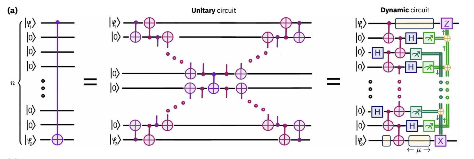
ดังที่แสดงในภาพ กระบวนการทำงานดังนี้:
- เตรียมห่วงโซ่ Bell pairs ที่เชื่อม Qubit ควบคุมกับ Qubit เป้าหมายผ่าน Qubit สำรองระหว่างกลาง
- ดำเนินการวัด Bell ระหว่าง Qubit เพื่อนบ้านที่ยังไม่พัวพัน โดยถ่ายทอดพัวพันทีละขั้นจนกว่า Qubit ควบคุมและ Qubit เป้าหมายจะแชร์ Bell pair กัน
- ใช้ Bell pair นี้สำหรับการเทเลพอร์ต Gate เพื่อแปลง CNOT แบบโลคอลให้กลายเป็น long-range CNOT แบบ deterministic ด้วยความลึกคงที่
วิธีนี้แทนที่ห่วงโซ่ SWAP ยาวด้วยโปรโตคอลความลึกคงที่ ลดการสัมผัสกับข้อผิดพลาดของ two-qubit gate และทำให้การดำเนินการสามารถขยายตามขนาดของอุปกรณ์ได้
ในส่วนต่อไป เราจะเริ่มต้นจากการอธิบายการนำ LRCX Circuit ไปใช้แบบ dynamic circuit ก่อน จากนั้นตอนท้ายจะให้การนำไปใช้แบบ unitary สำหรับเปรียบเทียบ เพื่อเน้นให้เห็นข้อดีของ dynamic circuits ในบริบทนี้
เริ่มต้น Circuit
เราเริ่มต้นด้วยปัญหาควอนตัมง่ายๆ ที่จะใช้เป็นฐานสำหรับการเปรียบเทียบ โดยเฉพาะคือ เราเริ่มต้น Circuit ด้วย Qubit ควบคุมที่ตำแหน่ง 0 และใช้ Hadamard Gate กับมัน ซึ่งจะสร้างสถานะซุปเปอร์โพซิชันที่เมื่อตามด้วยการดำเนินการ controlled-X จะสร้าง Bell state ระหว่าง Qubit ควบคุมกับ Qubit เป้าหมาย
ณ ขั้นตอนนี้ เรายังไม่ได้สร้าง long-range controlled-X (LRCX) เอง แต่เป้าหมายของเราคือการกำหนด Circuit เริ่มต้นที่ชัดเจนและกระชับซึ่งเน้นให้เห็นบทบาทของ LRCX ใน Step 2 เราจะแสดงให้เห็นว่า LRCX สามารถนำมาใช้เป็นการปรับปรุงโดยใช้ dynamic circuits ได้อย่างไร และเปรียบเทียบกับ unitary ที่เทียบเท่า สิ่งสำคัญคือโปรโตคอล LRCX สามารถนำไปใช้กับ Circuit เริ่มต้นใดก็ได้ ที่นี่เราใช้การตั้งค่า Hadamard ง่ายๆ นี้เพื่อความชัดเจนในการสาธิต
distance = 6  # The distance of the CNOT gate, with the convention that a distance of zero is a nearest-neighbor CNOT.

def initialize_circuit(distance):
    assert distance >= 0
    control = 0  # control qubit
    n = distance  # number of qubits between target and control

    qr = QuantumRegister(
        n + 2, name="q"
    )  # Circuit with n qubits between control and target
    cr = ClassicalRegister(
        2, name="cr"
    )  # Classical register for measuring control and target qubits

    k = int(n / 2)  # Number of Bell States to be used

    allcr = [cr]
    if (
        distance > 1
    ):  # This classical register will be used to store ZZ measurements.
        # It is only used for long-range CX gates with distance > 1
        c1 = ClassicalRegister(
            k, name="c1"
        )  # Classical register needed for post processing
        allcr.append(c1)
    if (
        distance > 0
    ):  # This classical register will be used to store XX measurements.
        # It is only used if distance > 0
        c2 = ClassicalRegister(
            n - k, name="c2"
        )  # Classical register needed for post processing
        allcr.append(c2)

    qc = QuantumCircuit(qr, *allcr, name="CNOT")

    # Apply a Hadamard gate to the control qubit such that the
    # long-range CNOT gate will prepare a
    # Bell state (|00> + |11>)/sqrt(2)
    qc.h(control)

    return qc

qc = initialize_circuit(distance)
qc.draw(fold=-1, output="mpl", scale=0.5)

ขั้นตอนที่ 2: ปรับปัญหาให้เหมาะสมสำหรับการรันบนฮาร์ดแวร์ควอนตัม
ในขั้นตอนนี้ เราจะแสดงวิธีสร้าง LRCX Circuit โดยใช้ dynamic circuits เป้าหมายคือการปรับ Circuit ให้เหมาะสมสำหรับการรันบนฮาร์ดแวร์โดยลดความลึกเมื่อเทียบกับการใช้ unitary ล้วนๆ เพื่อแสดงประโยชน์ เราจะแสดงทั้งโครงสร้าง LRCX แบบ dynamic และ unitary ที่เทียบเท่า แล้วเปรียบเทียบประสิทธิภาพหลังการ transpile สิ่งสำคัญคือ แม้ที่นี่เราจะใช้ LRCX กับปัญหาที่เริ่มต้นด้วย Hadamard ง่ายๆ แต่โปรโตคอลนี้สามารถนำไปใช้กับ Circuit ใดก็ได้ที่ต้องการ long-range CNOT
เตรียม Bell pairs
เราเริ่มต้นด้วยการสร้างห่วงโซ่ Bell pairs ตามเส้นทางระหว่าง Qubit ควบคุมกับ Qubit เป้าหมาย หากระยะทางเป็นคี่ เราจะใช้ CNOT จาก Qubit ควบคุมไปยังเพื่อนบ้านก่อน ซึ่งเป็น CNOT ที่จะถูกเทเลพอร์ต สำหรับระยะทางคู่ CNOT นี้จะถูกใช้หลังจากขั้นตอนการเตรียม Bell pair จากนั้นห่วงโซ่ Bell pair จะพัวพัน Qubit คู่ต่อเนื่องกัน ซึ่งสร้างทรัพยากรที่จำเป็นสำหรับการส่งข้อมูลควบคุมข้ามอุปกรณ์
# Determine where to start the Bell pair chain and add an extra CNOT when n is odd
def check_even(n: int) -> int:
    """Return 1 if n is even, else 2."""
    return 1 if n % 2 == 0 else 2

def prepare_bell_pairs(qc, add_barriers=True):
    n = qc.num_qubits - 2  # number of qubits between target and control
    k = int(n / 2)

    if add_barriers:
        qc.barrier()

    x0 = check_even(n)
    if n % 2 != 0:
        qc.cx(0, 1)

    # Create k Bell pairs
    for i in range(k):
        qc.h(x0 + 2 * i)
        qc.cx(x0 + 2 * i, x0 + 2 * i + 1)
    return qc

qc = prepare_bell_pairs(qc)
qc.draw(output="mpl", fold=-1, scale=0.5)

วัดคู่ Qubit เพื่อนบ้านในฐาน Bell
ถัดไป เราวัด Qubit เพื่อนบ้านที่ ยังไม่พัวพัน ในฐาน Bell (การวัด two-qubit ของ และ ) ซึ่งสร้าง Bell pair ระยะไกลระหว่าง Qubit เป้าหมายกับ Qubit ที่อยู่ติดกับ Qubit ควบคุม (ขึ้นอยู่กับการแก้ไข Pauli ซึ่งจะนำไปใช้ผ่าน feedforward ในขั้นตอนถัดไป) พร้อมกันนั้น เราใช้การวัดที่พัวพันซึ่งเทเลพอร์ต CNOT Gate ให้กระทำบน Qubit เป้าหมายที่ต้องการ
def measure_bell_basis(qc, add_barriers=True):
    n = qc.num_qubits - 2  # number of qubits between target and control
    k = int(n / 2)

    if n > 1:
        _, c1, c2 = qc.cregs
    elif n > 0:
        _, c2 = qc.cregs

    # Determine where to start the Bell pair chain and add an extra CNOT
    # when n is odd
    x0 = 1 if n % 2 == 0 else 2

    # Entangling layer that implements the Bell measurement
    # (and additionally adds the CNOT to be
    # teleported, if n is even)
    for i in range(k + 1):
        qc.cx(x0 - 1 + 2 * i, x0 + 2 * i)

    for i in range(1, k + x0):
        if i == 1:
            qc.h(2 * i + 1 - x0)
        else:
            qc.h(2 * i + 1 - x0)

    if add_barriers:
        qc.barrier()

    # Map the ZZ measurements onto classical register c1
    for i in range(k):
        if i == 0:
            qc.measure(2 * i + x0, c1[i])
        else:
            qc.measure(2 * i + x0, c1[i])

    # Map the XX measurements onto classical register c2
    for i in range(1, k + x0):
        if i == 1:
            qc.measure(2 * i + 1 - x0, c2[i - 1])
        else:
            qc.measure(2 * i + 1 - x0, c2[i - 1])
    return qc

qc = measure_bell_basis(qc)
qc.draw(output="mpl", fold=-1, scale=0.5)

ใช้การแก้ไข feedforward เพื่อแก้ไข Pauli byproduct operators
การวัดในฐาน Bell ทำให้เกิด Pauli byproducts ที่ต้องแก้ไขโดยใช้ผลการวัดที่บันทึกไว้ ซึ่งทำใน 2 ขั้นตอน ขั้นแรก เราต้องคำนวณค่า parity ของการวัด ทั้งหมด ซึ่งจะใช้เพื่อกำหนดเงื่อนไขการใช้ gate กับ Qubit เป้าหมาย ในทำนองเดียวกัน จะคำนวณค่า parity ของการวัด และใช้เพื่อกำหนดเงื่อนไขการใช้ gate กับ Qubit ควบคุม
ด้วย classical expression framework ใหม่ใน Qiskit ค่า parity เหล่านี้สามารถคำนวณได้โดยตรงใน classical processing layer ของ Circuit แทนที่จะใช้ลำดับของ conditional gate แต่ละตัวสำหรับแต่ละ bit ที่วัด เราสามารถสร้าง classical expression เดียวที่แทน XOR (parity) ของผลการวัดทั้งหมดที่เกี่ยวข้อง จากนั้น expression นี้จะถูกใช้เป็นเงื่อนไขใน if_test block เดียว ทำให้สามารถใช้ correction gate ในความลึกคงที่ได้ วิธีนี้ทั้งลดความซับซ้อนของ Circuit และรับประกันว่าการแก้ไข feedforward จะไม่เพิ่มเวลาแฝงที่ไม่จำเป็น
def apply_ffwd_corrections(qc):
    control = 0  # control qubit
    target = qc.num_qubits - 1  # target qubit
    n = qc.num_qubits - 2  # number of qubits between target and control

    k = int(n / 2)
    x0 = check_even(n)

    if n > 1:
        _, c1, c2 = qc.cregs
    elif n > 0:
        _, c2 = qc.cregs

    # First, let's compute the parity of all ZZ measurements
    for i in range(k):
        if i == 0:
            parity_ZZ = expr.lift(
                c1[i]
            )  # Store the value of the first ZZ measurement in parity_ZZ
        else:
            parity_ZZ = expr.bit_xor(
                c1[i], parity_ZZ
            )  # Successively compute the parity via XOR operations

    for i in range(1, k + x0):
        if i == 1:
            parity_XX = expr.lift(
                c2[i - 1]
            )  # Store the value of the first XX measurement in parity_XX
        else:
            parity_XX = expr.bit_xor(
                c2[i - 1], parity_XX
            )  # Successively compute the parity via XOR operations

    if n > 0:
        with qc.if_test(parity_XX):
            qc.z(control)

    if n > 1:
        with qc.if_test(parity_ZZ):
            qc.x(target)
    return qc

qc = apply_ffwd_corrections(qc)
qc.draw(output="mpl", fold=-1, scale=0.5)

วัด Qubit ควบคุมและ Qubit เป้าหมาย
เรากำหนด helper function ที่ช่วยให้สามารถวัด Qubit ควบคุมและ Qubit เป้าหมายในฐาน , หรือ ได้ สำหรับการตรวจสอบ Bell state ค่าที่คาดหวังของ และ ควรเป็น ทั้งคู่ เนื่องจากทั้งสองเป็น stabilizer ของสถานะนั้น การวัด ยังรองรับที่นี่และจะใช้ด้านล่างเมื่อคำนวณ fidelity
def measure_in_basis(qc, basis="XX", add_barrier=True):
    control = 0  # control qubit
    target = qc.num_qubits - 1  # target qubit

    assert basis in ["XX", "YY", "ZZ"]

    qc = (
        qc.copy()
    )  # We copy the circuit because we want to measure in different bases
    cr = qc.cregs[0]

    if add_barrier:
        qc.barrier()

    if basis == "XX":
        qc.h(control)
        qc.h(target)
    elif basis == "YY":
        qc.sdg(control)
        qc.sdg(target)
        qc.h(control)
        qc.h(target)

    qc.measure(control, cr[0])
    qc.measure(target, cr[1])
    return qc

qc_YY = measure_in_basis(qc.copy(), basis="YY")
qc_YY.draw(
    output="mpl", fold=-1, scale=0.5
)  # Circuit for measuring in the YY basis

รวมทุกอย่างเข้าด้วยกัน
เราผสมรวมขั้นตอนต่างๆ ที่กำหนดไว้ข้างต้นเพื่อสร้าง long-range CX Gate บนสองปลายของเส้นหนึ่งมิติ (1D) ขั้นตอนต่างๆ ได้แก่ดังนี้:
- เริ่มต้น Qubit ควบคุมใน
- เตรียม Bell pairs
- วัดคู่ Qubit เพื่อนบ้าน
- ใช้การแก้ไข feedforward ขึ้นอยู่กับ MCMs
def lrcx(distance, prep_barrier=True, pre_measure_barrier=True):
    qc = initialize_circuit(distance)
    qc = prepare_bell_pairs(qc, prep_barrier)
    qc = measure_bell_basis(qc, pre_measure_barrier)
    qc = apply_ffwd_corrections(qc)
    return qc

qc = lrcx(distance)
# Apply the measurement in the XX, YY, and ZZ bases
qc_XX, qc_YY, qc_ZZ = [
    measure_in_basis(qc, basis=basis) for basis in ["XX", "YY", "ZZ"]
]

qc_YY.draw(
    output="mpl", fold=-1, scale=0.5
)  # Circuit for measuring in the YY basis
การนำไปใช้แบบ unitary โดยการสลับ Qubit ไปยังกลาง
สำหรับการเปรียบเทียบ เราพิจารณาก่อนกรณีที่ long-range CNOT Gate ถูกนำไปใช้งานโดยใช้การเชื่อมต่อแบบ nearest-neighbor และ unitary gates ในภาพต่อไปนี้ ทางซ้ายคือ Circuit สำหรับ long-range CNOT gate ที่ครอบคลุมห่วงโซ่ 1D ของ n-qubits ภายใต้การเชื่อมต่อแบบ nearest-neighbor เท่านั้น ในตอนกลางคือการสลายตัวเชิง unitary ที่เทียบเท่าซึ่งนำไปใช้ได้ด้วย local CNOT gates, ความลึกของ Circuit
Circuit ในตอนกลางสามารถนำไปใช้ได้ดังนี้:
def cnot_unitary(distance):
    """Generate a long range CNOT gate using local CNOTs on a 1D
    chain of qubits subject to n
    nearest-neighbor connections only.

    Args:
        distance (int) : The distance of the CNOT gate,
        with the convention that
        a distance of 0 is a nearest-neighbor CNOT.

    Returns:
        QuantumCircuit: A Quantum Circuit implementing a
        long-range CNOT gate
        between qubit 0 and qubit distance+1
    """
    assert distance >= 0
    n = distance  # number of qubits between target and control

    qr = QuantumRegister(
        n + 2, name="q"
    )  # Circuit with n qubits between control and target
    cr = ClassicalRegister(
        2, name="cr"
    )  # Classical register for measuring control and target qubits

    qc = QuantumCircuit(qr, cr, name="CNOT_unitary")

    control_qubit = 0

    qc.h(control_qubit)  # Prepare the control qubit in the |+> state

    k = int(n / 2)
    qc.barrier()
    for i in range(control_qubit, control_qubit + k):
        qc.cx(i, i + 1)
        qc.cx(i + 1, i)
        qc.cx(-i - 1, -i - 2)
        qc.cx(-i - 2, -i - 1)
    if n % 2 == 1:
        qc.cx(k + 2, k + 1)
        qc.cx(k + 1, k + 2)
    qc.barrier()
    qc.cx(k, k + 1)
    for i in range(control_qubit, control_qubit + k):
        qc.cx(k - i, k - 1 - i)
        qc.cx(k - 1 - i, k - i)
        qc.cx(k + i + 1, k + i + 2)
        qc.cx(k + i + 2, k + i + 1)
    if n % 2 == 1:
        qc.cx(-2, -1)
        qc.cx(-1, -2)

    return qc

qc_uni = cnot_unitary(distance)
ตอนนี้สร้าง Circuit ที่วัดในฐาน , และ เช่นเดียวกับที่เราทำสำหรับ dynamic circuits ข้างต้น
# Apply the measurement in the XX, YY, and ZZ bases
qc_uni_XX, qc_uni_YY, qc_uni_ZZ = [
    measure_in_basis(qc_uni, basis=basis) for basis in ["XX", "YY", "ZZ"]
]

qc_uni_YY.draw(
    output="mpl", fold=-1, scale=0.5
)  # Circuit for measuring in the YY basis

ตอนนี้ที่เราสร้างทั้ง dynamic circuits และ unitary circuits สำหรับตัวอย่างขนาดเล็กที่ distance=6 แล้ว เราจะ transpile เพื่อรันบน simulator ที่ไม่มีสัญญาณรบกวนก่อน
from qiskit_aer import AerSimulator

aer_backend = AerSimulator()
pm_sim = generate_preset_pass_manager(
    optimization_level=0, backend=aer_backend
)

# Dynamic circuits
isa_sim_dyn = pm_sim.run([qc_XX, qc_YY, qc_ZZ])

# Unitary circuits
isa_sim_uni = pm_sim.run([qc_uni_XX, qc_uni_YY, qc_uni_ZZ])
ขั้นตอนที่ 3: รันโดยใช้ Qiskit primitives
ตอนนี้เราสามารถรันการทดลองบน noiseless simulator backend ได้แล้ว เราใช้ Qiskit Runtime Sampler กับ AerSimulator เป็น backend mode เพื่อรัน Circuit
sampler_sim = Sampler(mode=aer_backend)
sim_job = sampler_sim.run(isa_sim_dyn + isa_sim_uni)
sim_results = sim_job.result()
ขั้นตอนที่ 4: ประมวลผลและคืนผลลัพธ์ในรูปแบบคลาสสิกที่ต้องการ
หลังจากการทดลองรันเสร็จสิ้นแล้ว เราจะประมวลผลข้อมูลดิบจากการวัดเพื่อดึงเมตริกที่มีความหมาย ในขั้นตอนนี้ เราดำเนินการดังนี้:
- กำหนดเมตริกคุณภาพสำหรับประเมินประสิทธิภาพของ long-range CX
- คำนวณค่า expectation ของตัวดำเนินการ Pauli จากผลการวัดดิบ
- ใช้ค่าเหล่านี้เพื่อคำนวณ fidelity ของ Bell state ที่สร้างขึ้น
ในการจำลองที่ไม่มีสัญญาณรบกวน เราจะตรวจสอบว่าเมตริก fidelity เท่ากับ สำหรับ Circuit ที่สร้างขึ้น ในการทดลองบน QPU จริง การวิเคราะห์นี้จะให้ภาพที่ชัดเจนว่า dynamic circuits ทำงานได้ดีแค่ไหนเมื่อเทียบกับการนำไปใช้งานแบบ unitary baseline
เมตริกคุณภาพ
เพื่อประเมินความสำเร็จของโปรโตคอล long-range CX เราวัดว่า output state ใกล้เคียงกับ Bell state ในอุดมคติแค่ไหน วิธีที่สะดวกในการวัดปริมาณนี้คือการคำนวณ state fidelity โดยใช้ค่า expectation ของตัวดำเนินการ Pauli เราสามารถคำนวณ fidelity สำหรับ Bell state บน control และ target state หลังจากรู้ค่า , , และ โดยเฉพาะอย่างยิ่ง
เพื่อคำนวณค่า expectation เหล่านี้จากข้อมูลการวัดดิบ เราจะกำหนดฟังก์ชันช่วยเหลือชุดหนึ่ง:
compute_ZZ_expectation: รับ measurement counts แล้วคำนวณค่า expectation ของตัวดำเนินการ Pauli สอง Qubit ใน basiscompute_fidelity: รวมค่า expectation ของ , , และ เข้าสู่นิพจน์ fidelity ข้างต้นget_counts_from_bitarray: Utility สำหรับดึง counts จาก result object ของ Backend
def compute_ZZ_expectation(counts):
    total = sum(counts.values())
    expectation = 0
    for bitstring, count in counts.items():
        # Ensure bitstring is 2 bits
        z1 = (-1) ** (int(bitstring[-1]))
        z2 = (-1) ** (int(bitstring[-2]))
        expectation += z1 * z2 * count
    return expectation / total

def compute_fidelity(counts_xx, counts_yy, counts_zz):
    xx, yy, zz = [
        compute_ZZ_expectation(c) for c in [counts_xx, counts_yy, counts_zz]
    ]
    return 1 / 4 * (1 + xx - yy + zz)
# Dynamic fidelity
counts_xx = sim_results[0].data.cr.get_counts()
counts_yy = sim_results[1].data.cr.get_counts()
counts_zz = sim_results[2].data.cr.get_counts()
fidelity_dyn = compute_fidelity(counts_xx, counts_yy, counts_zz)

# Unitary fidelity
counts_xx = sim_results[3].data.cr.get_counts()
counts_yy = sim_results[4].data.cr.get_counts()
counts_zz = sim_results[5].data.cr.get_counts()
fidelity_uni = compute_fidelity(counts_xx, counts_yy, counts_zz)

print(f"Dynamic fidelity (distance={distance}): {fidelity_dyn:.4f}")
print(f"Unitary fidelity (distance={distance}): {fidelity_uni:.4f}")
Dynamic fidelity (distance=6): 1.0000
Unitary fidelity (distance=6): 1.0000
อย่างที่คาดไว้ในการจำลองที่ไม่มีสัญญาณรบกวน ค่า fidelity ทั้งใน dynamic circuits และ unitary circuits เท่ากับ
ตัวอย่างฮาร์ดแวร์ขนาดใหญ่
ที่นี่เราจะนำรายละเอียดทั้งหมดเหล่านี้มารวมกันเป็น workflow เดียวในระดับที่ใหญ่ขึ้น ซึ่งจะรันบนฮาร์ดแวร์ควอนตัมจริง
สร้าง Circuit สำหรับระยะทางต่างๆ
ตอนนี้เราสร้าง long-range CX circuits สำหรับช่วงของการแยก Qubit ได้ถึง 60 Qubit ห่างกัน สำหรับแต่ละระยะทาง เราสร้าง Circuit ที่วัดในฐาน , และ ซึ่งจะใช้ในภายหลังเพื่อคำนวณ fidelity
รายการระยะทางรวมทั้งการแยกระยะสั้นและยาว โดย distance = 0 สอดคล้องกับ nearest-neighbor CX ระยะทางเดียวกันนี้จะถูกใช้เพื่อสร้าง unitary circuits ที่สอดคล้องกันในภายหลังสำหรับการเปรียบเทียบ
# -------------------------Step 1-------------------------
distances = [
    0,
    1,
    2,
    3,
    6,
    11,
    16,
    21,
    28,
    35,
    44,
    55,
    60,
]  # Distances for long range CX. distance of 0 is a nearest-neighbor CX
distances.sort()
assert min(distances) >= 0
basis_list = ["XX", "YY", "ZZ"]

# Dynamic circuits
circuits_dyn = []
for distance in distances:
    for basis in basis_list:
        circuits_dyn.append(
            measure_in_basis(lrcx(distance, prep_barrier=False), basis=basis)
        )
print(f"Number of circuits: {len(circuits_dyn)}")

# Unitary circuits
circuits_uni = []
for distance in distances:
    for basis in basis_list:
        circuits_uni.append(
            measure_in_basis(cnot_unitary(distance), basis=basis)
        )

print(f"Number of circuits: {len(circuits_uni)}")
ตอนนี้ที่เรามี dynamic และ unitary circuits สำหรับช่วงระยะทางต่างๆ แล้ว เราพร้อมสำหรับการ transpile เราต้องเลือก backend device ก่อน
# -------------------------Step 2-------------------------
# Set up access to IBM Quantum devices
from qiskit.circuit import IfElseOp

service = QiskitRuntimeService()
backend = service.least_busy(
    operational=True, simulator=False, min_num_qubits=156
)
if "if_else" not in backend.target.operation_names:
    backend.target.add_instruction(IfElseOp, name="if_else")
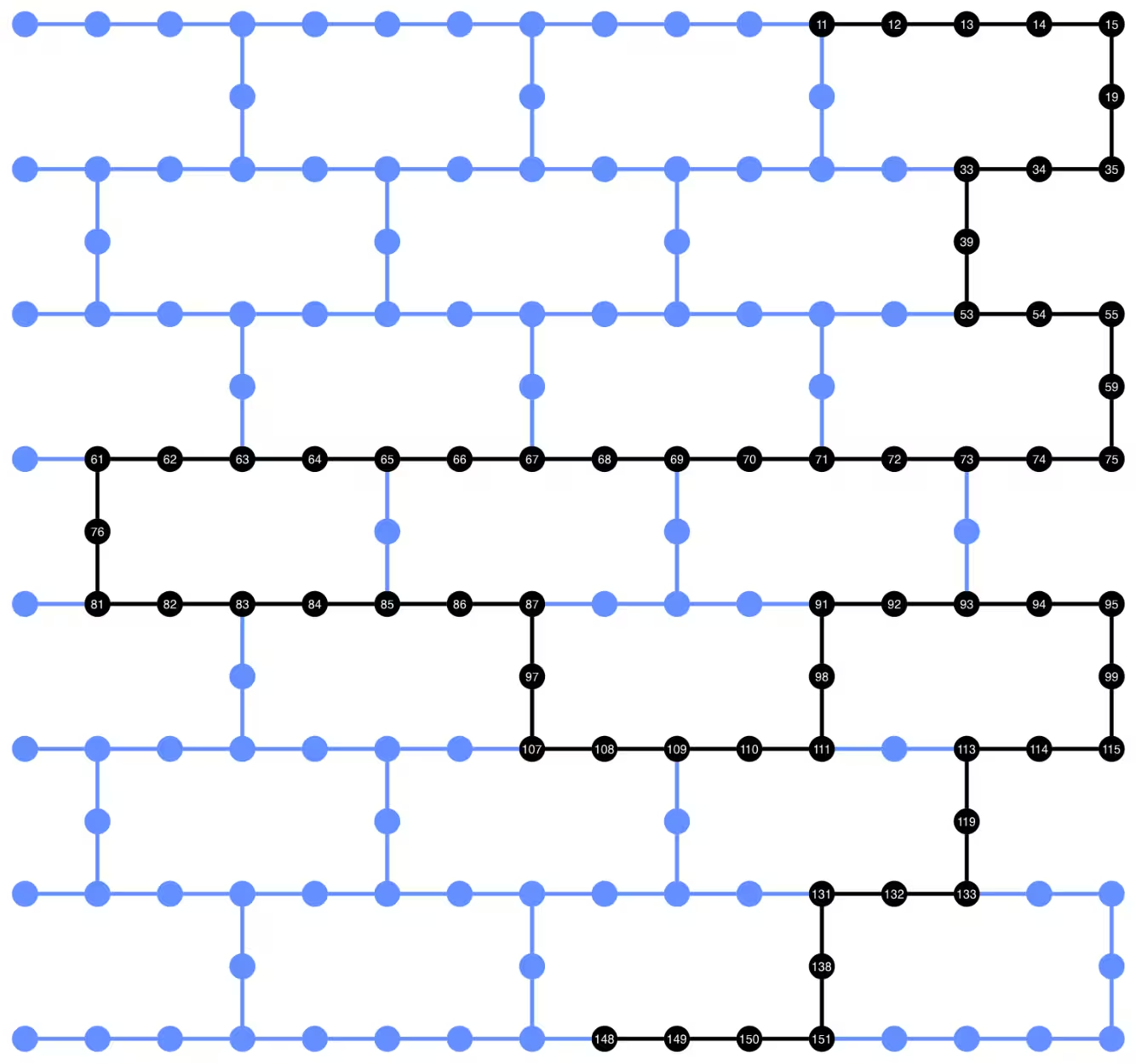
ใช้ Layer Fidelity string สำหรับการเลือก 1D chain
เนื่องจากเราต้องการเปรียบเทียบประสิทธิภาพของ dynamic circuit และ unitary circuit บน 1D chain เราจึงใช้ Layer Fidelity string เพื่อเลือกโทโพโลยีแบบเส้นตรงของ chain Qubit ที่ดีที่สุดจากอุปกรณ์ ซึ่งช่วยให้ Circuit ทั้งสองประเภทได้รับการ transpile ภายใต้ข้อจำกัดการเชื่อมต่อเดียวกัน ทำให้สามารถเปรียบเทียบประสิทธิภาพได้อย่างยุติธรรม
# This selects best qubits for longest distance and uses
# the same control for all lengths
lf_qubits = backend.properties().to_dict()[
    "general_qlists"
]  # best linear chain qubits
chosen_layouts = {
    distance: [
        val["qubits"]
        for val in lf_qubits
        if val["name"] == f"lf_{distances[-1] + 2}"
    ][0][: distance + 2]
    for distance in distances
}
print(chosen_layouts[max(distances)])  # best qubits at each distance
[11, 12, 13, 14, 15, 19, 35, 34, 33, 39, 53, 54, 55, 59, 75, 74, 73, 72, 71, 70, 69, 68, 67, 66, 65, 64, 63, 62, 61, 76, 81, 82, 83, 84, 85, 86, 87, 97, 107, 108, 109, 110, 111, 98, 91, 92, 93, 94, 95, 99, 115, 114, 113, 119, 133, 132, 131, 138, 151, 150, 149, 148]
isa_circuits_dyn = []
isa_circuits_uni = []

# Using the same initial layouts for both circuits for better
# apples to apples comparison
for qc in circuits_dyn:
    pm = generate_preset_pass_manager(
        optimization_level=1,
        backend=backend,
        initial_layout=chosen_layouts[qc.num_qubits - 2],
    )
    isa_circuits_dyn.append(pm.run(qc))

for qc in circuits_uni:
    pm = generate_preset_pass_manager(
        optimization_level=1,
        backend=backend,
        initial_layout=chosen_layouts[qc.num_qubits - 2],
    )
    isa_circuits_uni.append(pm.run(qc))
print(
f"2Q depth: "
f"{isa_circuits_dyn[14].depth(lambda x: x.operation.num_qubits == 2)}"
)
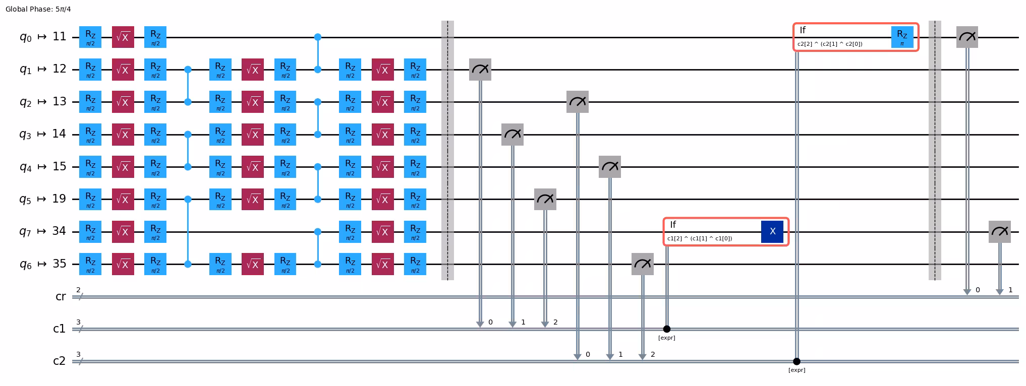
isa_circuits_dyn[14].draw("mpl", fold=-1, idle_wires=0)
Visualize qubits used for the LRCX circuit
ในส่วนนี้ เราจะตรวจสอบว่า LRCX Circuit ถูกแมปลงบนฮาร์ดแวร์อย่างไร เริ่มต้นด้วยการแสดงภาพ Physical Qubit ที่ใช้ใน Circuit จากนั้นศึกษาว่าระยะห่างระหว่าง Control และ Target ใน Layout ส่งผลต่อจำนวนการดำเนินการอย่างไร
2Q depth: 2
print(
f"2Q depth: "
f"{isa_circuits_uni[14].depth(lambda x: x.operation.num_qubits == 2)}"
)
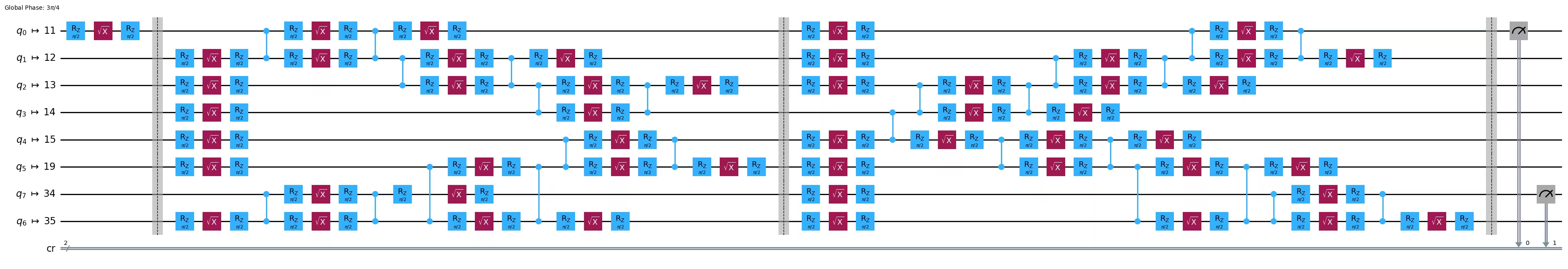
isa_circuits_uni[14].draw("mpl", fold=-1, idle_wires=False)
2Q depth: 13
ต่อไป เราจะรันการทดลองบน backend จริง นอกจากนี้ยังใช้การทำ batching เพื่อรันการทดลองข้ามหลาย trial ได้อย่างมีประสิทธิภาพ การรัน trial ซ้ำหลายครั้งช่วยให้คำนวณค่าเฉลี่ยได้ เพื่อเปรียบเทียบระหว่างวิธี unitary และ dynamic ได้แม่นยำยิ่งขึ้น รวมถึงวัดความแปรปรวนโดยเปรียบเทียบค่าเบี่ยงเบนในแต่ละ run
# Note: the qubit coordinates must be hard-coded.
# The backend API does not currently provide this information directly.
# If using a different backend, you will need to
# adjust the coordinates accordingly,
# or set the qubit_coordinates = None to use the default layout coordinates.

def _heron_coords_r2():
    """Generate coordinates for the Heron layout in R2. Note"""
    cord_map = np.array(
        [
            [
                0,
                1,
                2,
                3,
                4,
                5,
                6,
                7,
                8,
                9,
                10,
                11,
                12,
                13,
                14,
                15,
                3,
                7,
                11,
                15,
                0,
                1,
                2,
                3,
                4,
                5,
                6,
                7,
                8,
                9,
                10,
                11,
                12,
                13,
                14,
                15,
                1,
                5,
                9,
                13,
                0,
                1,
                2,
                3,
                4,
                5,
                6,
                7,
                8,
                9,
                10,
                11,
                12,
                13,
                14,
                15,
                3,
                7,
                11,
                15,
                0,
                1,
                2,
                3,
                4,
                5,
                6,
                7,
                8,
                9,
                10,
                11,
                12,
                13,
                14,
                15,
                1,
                5,
                9,
                13,
                0,
                1,
                2,
                3,
                4,
                5,
                6,
                7,
                8,
                9,
                10,
                11,
                12,
                13,
                14,
                15,
                3,
                7,
                11,
                15,
                0,
                1,
                2,
                3,
                4,
                5,
                6,
                7,
                8,
                9,
                10,
                11,
                12,
                13,
                14,
                15,
                1,
                5,
                9,
                13,
                0,
                1,
                2,
                3,
                4,
                5,
                6,
                7,
                8,
                9,
                10,
                11,
                12,
                13,
                14,
                15,
                3,
                7,
                11,
                15,
                0,
                1,
                2,
                3,
                4,
                5,
                6,
                7,
                8,
                9,
                10,
                11,
                12,
                13,
                14,
                15,
            ],
            -1
            * np.array([j for i in range(15) for j in [i] * [16, 4][i % 2]]),
        ],
        dtype=int,
    )

    hcords = []
    ycords = cord_map[0]
    xcords = cord_map[1]
    for i in range(156):
        hcords.append([xcords[i] + 1, np.abs(ycords[i]) + 1])

    return hcords

# Visualize the active qubits in the circuit layout
plot_circuit_layout(
    circuit=isa_circuits_uni[-1],
    backend=backend,
    view="physical",
    qubit_coordinates=_heron_coords_r2(),
)
# -------------------------Step 3-------------------------
num_trials = 10
jobs_uni = []
jobs_dyn = []
with Batch(backend=backend) as batch:
    sampler = Sampler(mode=batch)
    sampler.options.environment.job_tags = ["TUT_LRE"]
    for _ in range(num_trials):
        jobs_uni.append(sampler.run(isa_circuits_uni, shots=1024))
        jobs_dyn.append(sampler.run(isa_circuits_dyn, shots=1024))
เราคำนวณ fidelity สำหรับ dynamic long-range CX circuits สำหรับแต่ละระยะ เราดึงผลการวัดใน basis , , และ ผลลัพธ์เหล่านี้ถูกรวมเข้ากันโดยใช้ฟังก์ชันช่วยเหลือที่กำหนดไว้ก่อนหน้า เพื่อคำนวณ fidelity ตาม ซึ่งให้ค่า fidelity ที่สังเกตได้ของโปรโตคอลที่รันแบบ dynamic ในแต่ละระยะ
# -------------------------Step 4-------------------------
fidelities_dyn = []

# loop over trials
for job in jobs_dyn:
    result_dyn = job.result()
    trial_fidelities = []
    # loop over all distances
    for ind, dist in enumerate(distances):
        counts_xx = result_dyn[ind * 3].data.cr.get_counts()
        counts_yy = result_dyn[ind * 3 + 1].data.cr.get_counts()
        counts_zz = result_dyn[ind * 3 + 2].data.cr.get_counts()
        trial_fidelities.append(
            compute_fidelity(counts_xx, counts_yy, counts_zz)
        )
    fidelities_dyn.append(trial_fidelities)
# average over trials for each distance
avg_fidelities_dyn = np.mean(fidelities_dyn, axis=0)
std_fidelities_dyn = np.std(fidelities_dyn, axis=0)
ตอนนี้เราคำนวณ fidelity สำหรับ unitary long-range CX circuits โดยทำแบบเดียวกับที่ทำสำหรับ dynamic circuits ข้างต้น
fidelities_uni = []

# loop over trials
for job in jobs_uni:
    result_uni = job.result()
    trial_fidelities = []
    # loop over all distances
    for ind, dist in enumerate(distances):
        counts_xx = result_uni[ind * 3].data.cr.get_counts()
        counts_yy = result_uni[ind * 3 + 1].data.cr.get_counts()
        counts_zz = result_uni[ind * 3 + 2].data.cr.get_counts()
        trial_fidelities.append(
            compute_fidelity(counts_xx, counts_yy, counts_zz)
        )
    fidelities_uni.append(trial_fidelities)
# average over trials for each distance
avg_fidelities_uni = np.mean(fidelities_uni, axis=0)
std_fidelities_uni = np.std(fidelities_uni, axis=0)
Plot the results
เพื่อดูผลลัพธ์ในรูปแบบภาพ เซลล์ด้านล่างจะพล็อต gate fidelity ที่ประมาณไว้ซึ่งวัดได้ที่ระยะห่างต่างๆ ระหว่าง Qubit ที่พันกัน สำหรับแต่ละวิธี
fig, ax = plt.subplots()

# Unitary with error bars
ax.errorbar(
    distances,
    avg_fidelities_uni,
    yerr=std_fidelities_uni,
    fmt="o-.",
    color="c",
    ecolor="c",
    elinewidth=1,
    capsize=4,
    label="Unitary",
)
# Dynamic with error bars
ax.errorbar(
    distances,
    avg_fidelities_dyn,
    yerr=std_fidelities_dyn,
    fmt="o-.",
    color="m",
    ecolor="m",
    elinewidth=1,
    capsize=4,
    label="Dynamic",
)
# Random gate baseline
ax.axhline(y=1 / 4, linestyle="--", color="gray", label="Random gate")

legend = ax.legend(frameon=True)
for text in legend.get_texts():
    text.set_color("black")
legend.get_frame().set_facecolor("white")
legend.get_frame().set_edgecolor("black")
ax.set_title(
    "Bell State Fidelity vs Control–Target Separation", color="black"
)
ax.set_xlabel("Distance", color="black")
ax.set_ylabel("Bell state fidelity", color="black")
ax.grid(linestyle=":", linewidth=0.6, alpha=0.4, color="gray")
ax.set_ylim((0.2, 1))
ax.set_facecolor("white")
fig.patch.set_facecolor("white")
for spine in ax.spines.values():
    spine.set_visible(True)
    spine.set_color("black")
ax.tick_params(axis="x", colors="black")
ax.tick_params(axis="y", colors="black")
plt.show()
จากกราฟ fidelity ข้างต้น LRCX ไม่ได้ให้ผลดีกว่าการนำไปใช้งานแบบ unitary โดยตรงอย่างสม่ำเสมอ ในความเป็นจริง สำหรับระยะห่างระหว่าง Control และ Target ที่สั้น วิธี unitary circuit ให้ค่า fidelity สูงกว่า อย่างไรก็ตาม ที่ระยะห่างมากขึ้น dynamic circuit เริ่มให้ค่า fidelity ที่ดีกว่าวิธี unitary พฤติกรรมนี้ไม่ใช่เรื่องที่ไม่คาดคิดบนฮาร์ดแวร์ปัจจุบัน: แม้ว่า dynamic circuits จะลด circuit depth โดยหลีกเลี่ยง SWAP chain ที่ยาว แต่ก็แนะนำเวลา circuit เพิ่มเติมจาก mid-circuit measurements, classical feedforward, และความล่าช้าของ control-path การเพิ่ม latency ทำให้ decoherence และ readout errors เพิ่มขึ้น ซึ่งอาจมากกว่าประโยชน์ที่ได้จากการลด depth ที่ระยะสั้น
อย่างไรก็ตาม เราสังเกตเห็นจุดที่ dynamic approach แซงหน้า unitary นี่คือผลโดยตรงของ scaling ที่แตกต่างกัน: depth ของ unitary circuit เติบโตแบบเชิงเส้นตามระยะห่างระหว่าง Qubit ในขณะที่ depth ของ dynamic circuit คงที่
ประเด็นสำคัญ:
- ประโยชน์ทันทีของ dynamic circuits: แรงจูงใจหลักในปัจจุบันคือการลด two-qubit depth ไม่ใช่การปรับปรุง fidelity อย่างจำเป็น
- ทำไม fidelity อาจแย่กว่าในวันนี้: เวลา circuit ที่เพิ่มขึ้นจาก measurement และ classical operations มักจะครอบงำ โดยเฉพาะเมื่อระยะห่างระหว่าง Control และ Target น้อย
- มองไปข้างหน้า: เมื่อฮาร์ดแวร์ดีขึ้น โดยเฉพาะ readout ที่เร็วขึ้น, classical control latency ที่สั้นลง, และ mid-circuit overhead ที่ลดลง เราควรคาดหวังว่าการลด depth และ duration เหล่านี้จะแปลเป็นการเพิ่ม fidelity ที่วัดได้
# Compute metrics for each distance, skipping the basis circuits since
# they are identical for each distance
depths_2q_dyn = [
    c.depth(lambda x: x.operation.num_qubits == 2)
    for c in isa_circuits_dyn[::3]
]
meas_dyn = [
    sum(1 for instr in c.data if instr.operation.name == "measure")
    for c in isa_circuits_dyn[::3]
]

depths_2q_uni = [
    c.depth(lambda x: x.operation.num_qubits == 2)
    for c in isa_circuits_uni[::3]
]
meas_uni = [
    sum(1 for instr in c.data if instr.operation.name == "measure")
    for c in isa_circuits_uni[::3]
]

fig, axes = plt.subplots(1, 2, figsize=(12, 5))

axes[0].plot(
    distances, depths_2q_uni, "o-.", color="c", label="Unitary (2Q depth)"
)
axes[0].plot(
    distances, depths_2q_dyn, "o-.", color="m", label="Dynamic (2Q depth)"
)
axes[0].set_xlabel("Number of qubits between control and target")
axes[0].set_ylabel("Two-qubit depth")
axes[0].grid(True, linestyle=":", linewidth=0.6, alpha=0.4)
axes[0].legend()

axes[1].plot(
    distances, meas_uni, "o-.", color="c", label="Unitary (# measurements)"
)
axes[1].plot(
    distances, meas_dyn, "o-.", color="m", label="Dynamic (# measurements)"
)
axes[1].set_xlabel("Number of qubits between control and target")
axes[1].set_ylabel("Number of measurements")
axes[1].grid(True, linestyle=":", linewidth=0.6, alpha=0.4)
axes[1].legend()

fig.suptitle("Scaling of Unitary vs Dynamic LRCX with Distance", fontsize=12)

plt.tight_layout()
plt.show()
กราฟ two-qubit depth นี้เน้นให้เห็นข้อดีหลักของ LRCX ที่นำไปใช้ด้วย dynamic circuits: ประสิทธิภาพยังคงคงที่โดยพื้นฐานเมื่อระยะห่างระหว่าง control และ target Qubit เพิ่มขึ้น ในทางตรงกันข้าม วิธี unitary เติบโตแบบเชิงเส้นตามระยะห่างเนื่องจาก SWAP chain ที่จำเป็น Depth จับ logical scaling ของ two-qubit operations ในขณะที่ measurement count สะท้อน overhead เพิ่มเติมสำหรับ dynamic circuits การวัดเหล่านี้มีประสิทธิภาพ เนื่องจากดำเนินการแบบขนาน แต่ยังคงแนะนำต้นทุนคงที่บนฮาร์ดแวร์ในปัจจุบัน
ทำไม fidelity อาจแย่กว่าในวันนี้: เวลา circuit ที่เพิ่มขึ้นจาก measurement และ classical operations มักจะครอบงำ โดยเฉพาะเมื่อระยะห่างระหว่าง control-target น้อย ตัวอย่างเช่น ความยาว readout เฉลี่ยบน Heron r2 processor คือ 2,280 ns ในขณะที่ความยาว 2Q gate มีเพียง 68 ns เท่านั้น
เมื่อ measurement และ classical latencies ดีขึ้น เราคาดว่า constant-depth และ constant-measurement scaling ของ dynamic circuits จะให้ข้อได้เปรียบด้าน fidelity และ runtime ที่ชัดเจนบน circuit ขนาดใหญ่
ขั้นตอนถัดไป
หากคุณพบว่างานนี้น่าสนใจ คุณอาจสนใจสื่อต่อไปนี้:
References
[1] Efficient Long-Range Entanglement using Dynamic Circuits, by Elisa Bäumer, Vinay Tripathi, Derek S. Wang, Patrick Rall, Edward H. Chen, Swarnadeep Majumder, Alireza Seif, Zlatko K. Minev. IBM Quantum, (2023).