การจำลอง Kicked Ising Hamiltonian ด้วย Dynamic Circuits

ประมาณการการใช้งาน: 7.5 นาทีบนโปรเซสเซอร์ Heron r3 (หมายเหตุ: นี่เป็นเพียงการประมาณเท่านั้น เวลาจริงอาจแตกต่างกัน) Dynamic circuits คือ Circuit ที่มีการป้อนข้อมูลแบบ classical feedforward กล่าวคือ เป็นการวัดกลางวงจร (mid-circuit measurement) ตามด้วยการดำเนินการทางตรรกะแบบคลาสสิกที่กำหนดการดำเนินการควอนตัมโดยขึ้นอยู่กับผลลัพธ์คลาสสิก ในบทแนะนำนี้ เราจำลองแบบจำลอง kicked Ising บน lattice หกเหลี่ยมของ spin และใช้ dynamic circuits เพื่อสร้างปฏิสัมพันธ์ที่อยู่นอกเหนือการเชื่อมต่อทางกายภาพของฮาร์ดแวร์

แบบจำลอง Ising ได้รับการศึกษาอย่างกว้างขวางในด้านฟิสิกส์หลายสาขา มันจำลอง spin ที่มีปฏิสัมพันธ์แบบ Ising ระหว่างไซต์บน lattice รวมถึงการเตะ (kick) จากสนามแม่เหล็กเฉพาะที่บนแต่ละไซต์ การวิวัฒน์เวลาแบบ Trotterized ของ spin ที่พิจารณาในบทแนะนำนี้ นำมาจาก [1] และแสดงด้วย unitary ดังต่อไปนี้:

$$U(\theta)=\left(\prod_{\langle j, k\rangle} \exp \left(i \frac{\pi}{8} Z_j Z_k\right)\right)\left(\prod_j \exp \left(-i \frac{\theta}{2} X_j\right)\right)$$

เพื่อตรวจสอบพลวัตของ spin เราศึกษาค่าแมกเนไทเซชันเฉลี่ยของ spin ที่แต่ละไซต์เป็นฟังก์ชันของ Trotter steps ดังนั้นเราจึงสร้าง observable ดังต่อไปนี้:

$$\langle O\rangle = \frac{1}{N} \sum_i \langle Z_i \rangle$$

เพื่อสร้างปฏิสัมพันธ์ ZZ ระหว่างไซต์บน lattice เราเสนอวิธีแก้ปัญหาโดยใช้ฟีเจอร์ dynamic circuit ซึ่งทำให้ความลึกของ two-qubit สั้นลงอย่างมีนัยสำคัญเมื่อเทียบกับวิธีการ routing มาตรฐานที่ใช้ SWAP gates อย่างไรก็ตาม การดำเนินการ classical feedforward ใน dynamic circuits มักใช้เวลาในการดำเนินการนานกว่า quantum gates ดังนั้น dynamic circuits จึงมีข้อจำกัดและการแลกเปลี่ยนบางอย่าง นอกจากนี้เรายังนำเสนอวิธีการเพิ่มลำดับ dynamical decoupling บน qubit ที่อยู่นิ่ง (idling) ระหว่างการดำเนินการ classical feedforward โดยใช้ระยะเวลา stretch

ข้อกำหนด

ก่อนเริ่มบทแนะนำนี้ ต้องมีสิ่งต่อไปนี้ติดตั้งไว้:

• Qiskit SDK v2.0 หรือใหม่กว่า พร้อมรองรับ visualization
• Qiskit Runtime v0.37 หรือใหม่กว่า พร้อมรองรับ visualization (pip install 'qiskit-ibm-runtime[visualization]')
• ไลบรารีกราฟ Rustworkx (pip install rustworkx)
• Qiskit Aer (pip install qiskit-aer)

ตั้งค่า

# Added by doQumentation — required packages for this notebook
!pip install -q matplotlib numpy qiskit qiskit-aer qiskit-ibm-runtime rustworkx

import numpy as np
from typing import List
import rustworkx as rx
import matplotlib.pyplot as plt
from rustworkx.visualization import mpl_draw
from qiskit.circuit import (
    Parameter,
    QuantumCircuit,
    QuantumRegister,
    ClassicalRegister,
)
from qiskit.transpiler import CouplingMap
from qiskit.quantum_info import SparsePauliOp
from qiskit.circuit.classical import expr
from qiskit.transpiler.preset_passmanagers import (
    generate_preset_pass_manager,
)
from qiskit.transpiler import PassManager
from qiskit.circuit.library import RZGate, XGate
from qiskit.transpiler.passes import (
    ALAPScheduleAnalysis,
    PadDynamicalDecoupling,
)

from qiskit.transpiler.basepasses import TransformationPass
from qiskit.circuit.measure import Measure
from qiskit.transpiler.passes.utils.remove_final_measurements import (
    calc_final_ops,
)
from qiskit.circuit import Instruction

from qiskit.visualization import plot_circuit_layout
from qiskit.circuit.tools import pi_check

from qiskit_aer import AerSimulator
from qiskit_aer.primitives import SamplerV2 as Aer_Sampler

from qiskit_ibm_runtime import (
    QiskitRuntimeService,
    Batch,
    SamplerV2 as Sampler,
)
from qiskit_ibm_runtime.exceptions import QiskitBackendNotFoundError
from qiskit_ibm_runtime.visualization import (
    draw_circuit_schedule_timing,
)

ขั้นตอนที่ 1: แปลง input แบบคลาสสิกเป็น quantum circuit

เราเริ่มด้วยการกำหนด lattice ที่จะจำลอง เราเลือกทำงานกับ lattice แบบรังผึ้ง (honeycomb) หรือที่เรียกว่า lattice หกเหลี่ยม ซึ่งเป็นกราฟระนาบที่มี node ระดับ 3 ที่นี่เราระบุขนาดของ lattice และพารามิเตอร์ Circuit ที่เกี่ยวข้องในพลวัตแบบ Trotterized เราจำลองวิวัฒน์เวลาแบบ Trotterized ภายใต้แบบจำลอง Ising โดยใช้ค่า $\theta$ สามค่าของสนามแม่เหล็กเฉพาะที่

hex_rows = 3  # specify lattice size
hex_cols = 5
depths = range(9)  # specify Trotter steps
zz_angle = np.pi / 8  # parameter for ZZ interaction
max_angle = np.pi / 2  # max theta angle
points = 3  # number of theta parameters

θ = Parameter("θ")
params = np.linspace(0, max_angle, points)

def make_hex_lattice(hex_rows=1, hex_cols=1):
    """Define hexagon lattice."""
    hex_cmap = CouplingMap.from_hexagonal_lattice(
        hex_rows, hex_cols, bidirectional=False
    )
    data = list(hex_cmap.physical_qubits)
    graph = hex_cmap.graph.to_undirected(multigraph=False)
    edge_colors = rx.graph_misra_gries_edge_color(graph)
    layer_edges = {color: [] for color in edge_colors.values()}
    for edge_index, color in edge_colors.items():
        layer_edges[color].append(graph.edge_list()[edge_index])
    return data, layer_edges, hex_cmap, graph

มาเริ่มด้วยตัวอย่างทดสอบขนาดเล็ก:

hex_rows_test = 1
hex_cols_test = 2

data_test, layer_edges_test, hex_cmap_test, graph_test = make_hex_lattice(
    hex_rows=hex_rows_test, hex_cols=hex_cols_test
)

# display a small example for illustration
node_colors_test = ["lightblue"] * len(graph_test.node_indices())
pos = rx.graph_spring_layout(
    graph_test,
    k=5 / np.sqrt(len(graph_test.nodes())),
    repulsive_exponent=1,
    num_iter=150,
)
mpl_draw(graph_test, node_color=node_colors_test, pos=pos)

เราจะใช้ตัวอย่างขนาดเล็กนี้สำหรับการแสดงและการจำลอง ด้านล่างเราสร้างตัวอย่างขนาดใหญ่เพื่อแสดงว่า workflow สามารถขยายไปสู่ขนาดที่ใหญ่ขึ้นได้

data, layer_edges, hex_cmap, graph = make_hex_lattice(
    hex_rows=hex_rows, hex_cols=hex_cols
)
num_qubits = len(data)
print(f"num_qubits = {num_qubits}")

# display the honeycomb lattice to simulate
node_colors = ["lightblue"] * len(graph.node_indices())
pos = rx.graph_spring_layout(
    graph,
    k=5 / np.sqrt(num_qubits),
    repulsive_exponent=1,
    num_iter=150,
)
mpl_draw(graph, node_color=node_colors, pos=pos)
plt.show()

num_qubits = 46

สร้าง unitary circuits

เมื่อกำหนดขนาดของปัญหาและพารามิเตอร์แล้ว ตอนนี้เราพร้อมที่จะสร้าง Circuit แบบ parametrized ที่จำลองวิวัฒน์เวลาแบบ Trotterized ของ $U(\theta)$ ด้วย Trotter steps ต่างๆ ซึ่งระบุโดย argument depth Circuit ที่เราสร้างมีเลเยอร์สลับกันของ Rx($\theta$) gates และ Rzz gates โดยที่ Rzz gates สร้างปฏิสัมพันธ์ ZZ ระหว่าง spin ที่เชื่อมต่อกัน ซึ่งจะถูกวางระหว่างไซต์แต่ละคู่บน lattice ที่ระบุโดย argument layer_edges

def gen_hex_unitary(
    num_qubits=6,
    zz_angle=np.pi / 8,
    layer_edges=[
        [(0, 1), (2, 3), (4, 5)],
        [(1, 2), (3, 4), (5, 0)],
    ],
    θ=Parameter("θ"),
    depth=1,
    measure=False,
    final_rot=True,
):
    """Build unitary circuit."""
    circuit = QuantumCircuit(num_qubits)
    # Build trotter layers
    for _ in range(depth):
        for i in range(num_qubits):
            circuit.rx(θ, i)
        circuit.barrier()
        for coloring in layer_edges.keys():
            for e in layer_edges[coloring]:
                circuit.rzz(zz_angle, e[0], e[1])
        circuit.barrier()
    # Optional final rotation, set True to be consistent with Ref. [1]
    if final_rot:
        for i in range(num_qubits):
            circuit.rx(θ, i)
    if measure:
        circuit.measure_all()

    return circuit

แสดง Circuit ทดสอบขนาดเล็ก:

circ_unitary_test = gen_hex_unitary(
    num_qubits=len(data_test),
    layer_edges=layer_edges_test,
    θ=Parameter("θ"),
    depth=1,
    measure=True,
)
circ_unitary_test.draw(output="mpl", fold=-1)

ในทำนองเดียวกัน สร้าง unitary circuits ของตัวอย่างขนาดใหญ่ที่ Trotter steps ต่างๆ และ observable สำหรับประมาณค่าความคาดหวัง

circuits_unitary = []
for depth in depths:
    circ = gen_hex_unitary(
        num_qubits=num_qubits,
        layer_edges=layer_edges,
        θ=Parameter("θ"),
        depth=depth,
        measure=True,
    )
    circuits_unitary.append(circ)

observables_unitary = SparsePauliOp.from_sparse_list(
    [("Z", [i], 1 / num_qubits) for i in range(num_qubits)],
    num_qubits=num_qubits,
)

สร้างการใช้งาน dynamic circuit

ส่วนนี้สาธิตการใช้งาน dynamic circuit หลักเพื่อจำลองวิวัฒน์เวลาแบบ Trotterized เดียวกัน โปรดทราบว่า lattice รังผึ้งที่เราต้องการจำลองไม่ตรงกับ heavy lattice ของ qubit ในฮาร์ดแวร์ วิธีง่ายๆ ในการแมป Circuit ไปยังฮาร์ดแวร์คือการแนะนำชุดของการดำเนินการ SWAP เพื่อนำ qubit ที่มีปฏิสัมพันธ์มาอยู่ใกล้กัน เพื่อสร้างปฏิสัมพันธ์ ZZ ที่นี่เราเน้นแนวทางอื่นโดยใช้ dynamic circuits เป็นวิธีแก้ปัญหา ซึ่งแสดงให้เห็นว่าเราสามารถใช้การผสมผสานระหว่างการคำนวณควอนตัมและคลาสสิกแบบ real-time ภายใน Circuit ใน Qiskit เพื่อสร้างปฏิสัมพันธ์ที่อยู่นอกเหนือเพื่อนบ้านที่ใกล้ที่สุด

ในการใช้งาน dynamic circuit นั้น ปฏิสัมพันธ์ ZZ ถูกนำไปใช้อย่างมีประสิทธิภาพโดยใช้ ancilla qubits, การวัดกลางวงจร (mid-circuit measurement) และ feedforward เพื่อทำความเข้าใจสิ่งนี้ โปรดทราบว่า ZZ rotations ใช้ปัจจัยเฟส $e^{i\theta}$ กับสถานะตาม parity สำหรับสอง qubit สถานะ basis การคำนวณคือ $|00\rangle$, $|01\rangle$, $|10\rangle$, และ $|11\rangle$ ZZ rotation gate ใช้ปัจจัยเฟสกับสถานะ $|01\rangle$ และ $|10\rangle$ ซึ่งมี parity (จำนวนของ ones ในสถานะ) เป็นคี่ และปล่อยสถานะ parity คู่ไม่เปลี่ยนแปลง ต่อไปนี้อธิบายวิธีที่เราสามารถนำปฏิสัมพันธ์ ZZ ไปใช้กับสอง qubit อย่างมีประสิทธิภาพโดยใช้ dynamic circuits

1. คำนวณ parity ลงใน ancilla qubit: แทนที่จะใช้ ZZ กับสอง qubit โดยตรง เราแนะนำ qubit ที่สาม ซึ่งเป็น ancilla qubit เพื่อเก็บข้อมูล parity ของ data qubits ทั้งสอง เราพัน ancilla กับ data qubit แต่ละตัวโดยใช้ CX gates จาก data qubit ไปยัง ancilla qubit

2. ใช้การหมุน Z แบบ single-qubit กับ ancilla qubit: เนื่องจาก ancilla มีข้อมูล parity ของ data qubits ทั้งสอง ซึ่งนำไปใช้ ZZ rotation บน data qubits อย่างมีประสิทธิภาพ

3. วัด ancilla qubit ใน X basis: นี่คือขั้นตอนสำคัญที่ทำให้สถานะของ ancilla qubit ยุบตัว และผลลัพธ์การวัดบอกเราว่าเกิดอะไรขึ้น:

   • วัดได้ 0: เมื่อสังเกตผลลัพธ์ 0 เราได้ใช้ rotation $ZZ(\theta)$ กับ data qubits อย่างถูกต้องแล้ว

   • วัดได้ 1: เมื่อสังเกตผลลัพธ์ 1 เราได้ใช้ $ZZ(\theta + \pi)$ แทน

4. ใช้ correction gate เมื่อวัดได้ 1: ถ้าเราวัดได้ 1 เราใช้ Z gates กับ data qubits เพื่อ "แก้ไข" เฟส $\pi$ ที่เพิ่มมา

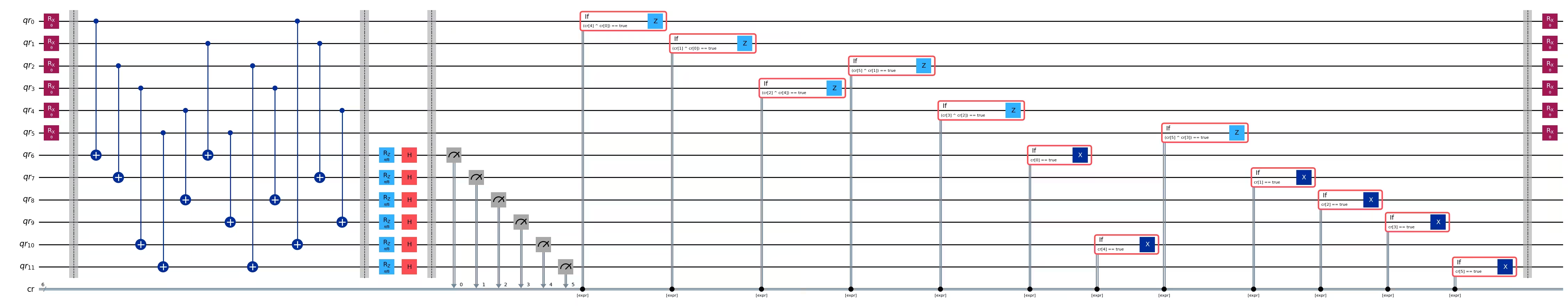
Circuit ที่ได้คือดังต่อไปนี้:

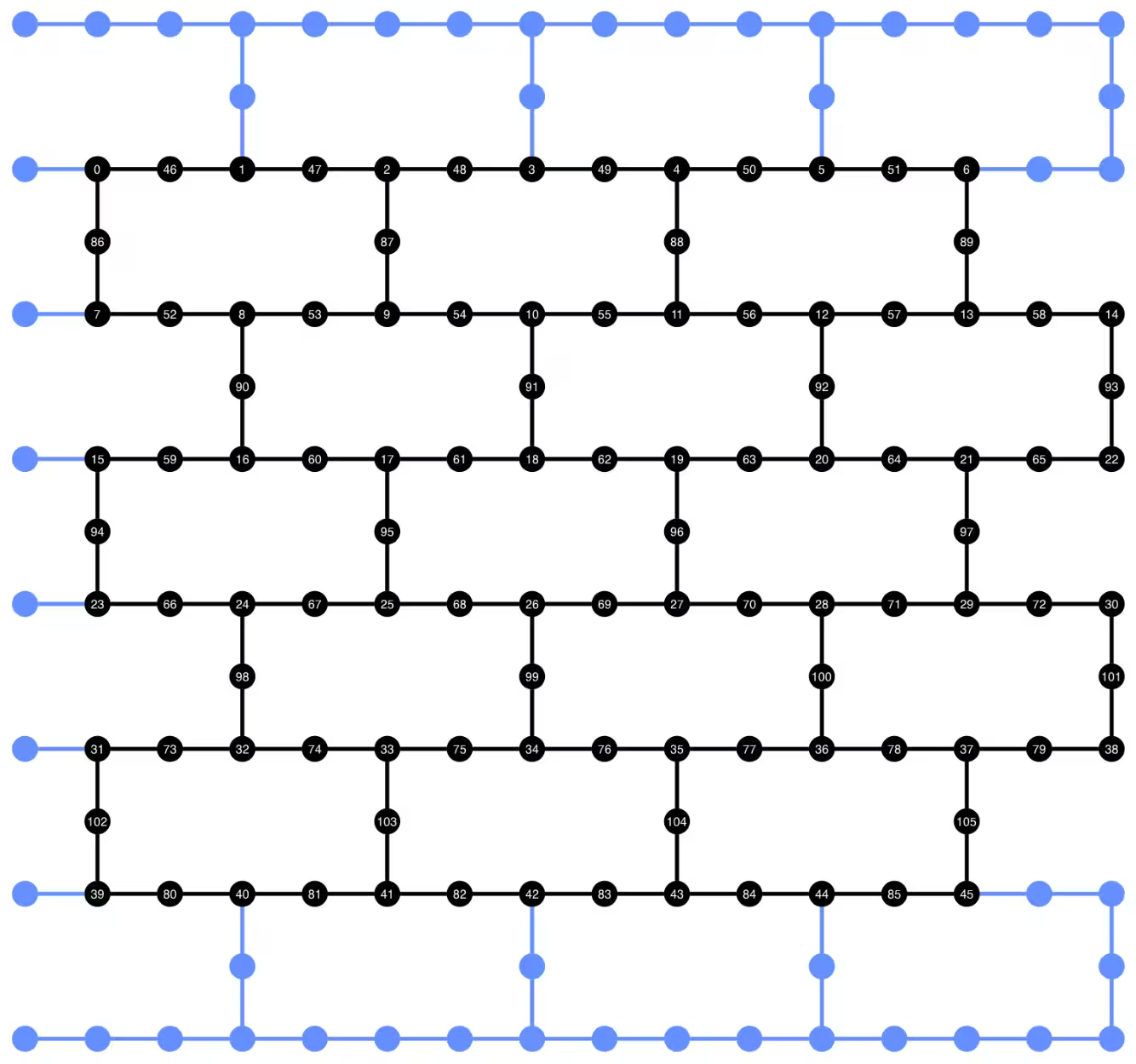
เมื่อเราใช้แนวทางนี้เพื่อจำลอง lattice รังผึ้ง Circuit ที่ได้จะฝังตัวเข้ากับฮาร์ดแวร์ heavy-hex lattice ได้อย่างสมบูรณ์แบบ: data qubits ทั้งหมดอยู่บนไซต์ระดับ 3 ของ lattice ซึ่งก่อให้เกิด lattice หกเหลี่ยม ทุกคู่ของ data qubits มี ancilla qubit ร่วมกันซึ่งอยู่บนไซต์ระดับ 2 ด้านล่าง เราสร้าง qubit lattice สำหรับการใช้งาน dynamic circuit โดยแนะนำ ancilla qubits (แสดงด้วยวงกลมสีม่วงเข้ม)

def make_lattice(hex_rows=1, hex_cols=1):
    """Define heavy-hex lattice and corresponding lists of data and ancilla nodes."""
    hex_cmap = CouplingMap.from_hexagonal_lattice(
        hex_rows, hex_cols, bidirectional=False
    )
    data = list(hex_cmap.physical_qubits)

    heavyhex_cmap = CouplingMap()
    for d in data:
        heavyhex_cmap.add_physical_qubit(d)

    # make coupling map
    a = len(data)
    for edge in hex_cmap.get_edges():
        heavyhex_cmap.add_physical_qubit(a)
        heavyhex_cmap.add_edge(edge[0], a)
        heavyhex_cmap.add_edge(edge[1], a)
        a += 1
    ancilla = list(range(len(data), a))
    qubits = data + ancilla

    # color edges
    graph = heavyhex_cmap.graph.to_undirected(multigraph=False)
    edge_colors = rx.graph_misra_gries_edge_color(graph)
    layer_edges = {color: [] for color in edge_colors.values()}
    for edge_index, color in edge_colors.items():
        layer_edges[color].append(graph.edge_list()[edge_index])

    # construct observable
    obs_hex = SparsePauliOp.from_sparse_list(
        [("Z", [i], 1 / len(data)) for i in data],
        num_qubits=len(qubits),
    )

    return (data, qubits, ancilla, layer_edges, heavyhex_cmap, graph, obs_hex)

แสดง heavy-hex lattice สำหรับ data qubits และ ancilla qubits ในขนาดเล็ก:

(data, qubits, ancilla, layer_edges, heavyhex_cmap, graph, obs_hex) = (
    make_lattice(hex_rows=hex_rows, hex_cols=hex_cols)
)

print(f"number of data qubits = {len(data)}")
print(f"number of ancilla qubits = {len(ancilla)}")

node_colors = []
for node in graph.node_indices():
    if node in ancilla:
        node_colors.append("purple")
    else:
        node_colors.append("lightblue")

pos = rx.graph_spring_layout(
    graph,
    k=1 / np.sqrt(len(qubits)),
    repulsive_exponent=2,
    num_iter=200,
)

# Visualize the graph, blue circles are data qubits and purple circles are ancillas
mpl_draw(graph, node_color=node_colors, pos=pos)
plt.show()

number of data qubits = 46
number of ancilla qubits = 60

ด้านล่าง เราสร้าง dynamic circuit สำหรับวิวัฒน์เวลาแบบ Trotterized โดย RZZ gates ถูกแทนที่ด้วยการใช้งาน dynamic circuit โดยใช้ขั้นตอนที่อธิบายไว้ข้างต้น

def gen_hex_dynamic(
    depth=1,
    zz_angle=np.pi / 8,
    θ=Parameter("θ"),
    hex_rows=1,
    hex_cols=1,
    measure=False,
    add_dd=True,
):
    """Build dynamic circuits."""
    (data, qubits, ancilla, layer_edges, heavyhex_cmap, graph, obs_hex) = (
        make_lattice(hex_rows=hex_rows, hex_cols=hex_cols)
    )
    # Initialize circuit
    qr = QuantumRegister(len(qubits), "qr")
    cr = ClassicalRegister(len(ancilla), "cr")
    circuit = QuantumCircuit(qr, cr)

    for k in range(depth):
        # Single-qubit Rx layer
        for d in data:
            circuit.rx(θ, d)
        circuit.barrier()

        # CX gates from data qubits to ancilla qubits
        for same_color_edges in layer_edges.values():
            for e in same_color_edges:
                circuit.cx(e[0], e[1])
        circuit.barrier()

        # Apply Rz rotation on ancilla qubits and rotate into X basis
        for a in ancilla:
            circuit.rz(zz_angle, a)
            circuit.h(a)
        # Add barrier to align terminal measurement
        circuit.barrier()

        # Measure ancilla qubits
        for i, a in enumerate(ancilla):
            circuit.measure(a, i)
        d2ros = {}
        a2ro = {}
        # Retrieve ancilla measurement outcomes
        for a in ancilla:
            a2ro[a] = cr[ancilla.index(a)]

        # For each data qubit, retrieve measurement outcomes of neighboring ancilla qubits
        for d in data:
            ros = [a2ro[a] for a in heavyhex_cmap.neighbors(d)]
            d2ros[d] = ros

        # Build classical feedforward operations (optionally add DD on idling data qubits)
        for d in data:
            if add_dd:
                circuit = add_stretch_dd(circuit, d, f"data_{d}_depth_{k}")

            # # XOR the neighboring readouts of the data qubit; if True, apply Z to it
            ros = d2ros[d]
            parity = ros[0]
            for ro in ros[1:]:
                parity = expr.bit_xor(parity, ro)
            with circuit.if_test(expr.equal(parity, True)):
                circuit.z(d)

        # Reset the ancilla if its readout is 1
        for a in ancilla:
            with circuit.if_test(expr.equal(a2ro[a], True)):
                circuit.x(a)
        circuit.barrier()

    # Final single-qubit Rx layer to match the unitary circuits
    for d in data:
        circuit.rx(θ, d)

    if measure:
        circuit.measure_all()
    return circuit, obs_hex

def add_stretch_dd(qc, q, name):
    """Add XpXm DD sequence."""
    s = qc.add_stretch(name)
    qc.delay(s, q)
    qc.x(q)
    qc.delay(s, q)
    qc.delay(s, q)
    qc.rz(np.pi, q)
    qc.x(q)
    qc.rz(-np.pi, q)
    qc.delay(s, q)
    return qc

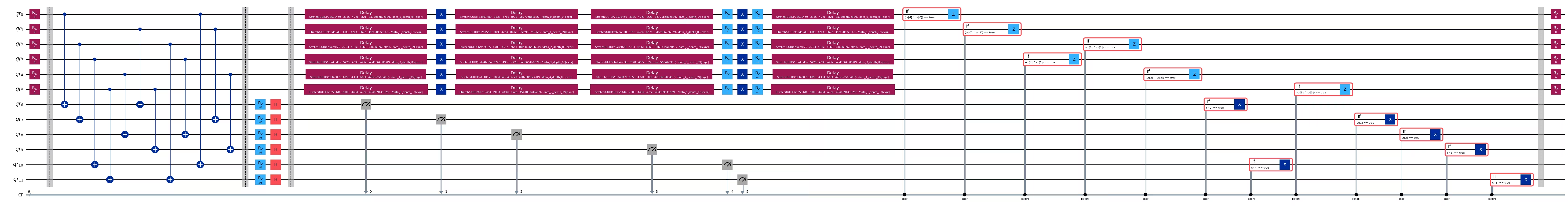
Dynamical decoupling (DD) และการรองรับระยะเวลา stretch

ข้อเสียอย่างหนึ่งของการใช้งาน dynamic circuit เพื่อสร้างปฏิสัมพันธ์ ZZ คือ การวัดกลางวงจรและการดำเนินการ classical feedforward มักใช้เวลานานกว่า quantum gates ในการดำเนินการ เพื่อระงับการ decoherence ของ qubit ระหว่างเวลาที่อยู่นิ่งสำหรับการดำเนินการคลาสสิก เราเพิ่มลำดับ dynamical decoupling (DD) หลังจากการดำเนินการวัดบน ancilla qubits และก่อนการดำเนินการ conditional Z บน data qubit ก่อนคำสั่ง if_test

ลำดับ DD ถูกเพิ่มโดยฟังก์ชัน add_stretch_dd() ซึ่งใช้ ระยะเวลา stretch เพื่อกำหนดช่วงเวลาระหว่าง DD gates ระยะเวลา stretch เป็นวิธีการระบุระยะเวลาแบบยืดหยุ่นสำหรับการดำเนินการ delay เพื่อให้ระยะเวลาของ delay สามารถขยายเพื่อเติมเต็มเวลาที่ qubit อยู่นิ่ง ตัวแปรระยะเวลาที่ระบุโดย stretch ถูกแก้ไขในเวลา compile เป็นระยะเวลาที่ต้องการซึ่งตอบสนองข้อจำกัดบางอย่าง สิ่งนี้มีประโยชน์มากเมื่อ timing ของลำดับ DD มีความสำคัญเพื่อให้ได้ประสิทธิภาพการระงับข้อผิดพลาดที่ดี สำหรับรายละเอียดเพิ่มเติมเกี่ยวกับประเภท stretch ดูเอกสาร OpenQASM ในปัจจุบัน การรองรับประเภท stretch ใน Qiskit Runtime ยังอยู่ในขั้นทดลอง สำหรับรายละเอียดเกี่ยวกับข้อจำกัดการใช้งาน โปรดดูส่วนข้อจำกัด ของเอกสาร stretch

โดยใช้ฟังก์ชันที่กำหนดไว้ข้างต้น เราสร้าง Circuit วิวัฒน์เวลาแบบ Trotterized ทั้งแบบมีและไม่มี DD และ observables ที่สอดคล้องกัน เราเริ่มด้วยการแสดง dynamic circuit ของตัวอย่างขนาดเล็ก:

hex_rows_test = 1
hex_cols_test = 1

(
    data_test,
    qubits_test,
    ancilla_test,
    layer_edges_test,
    heavyhex_cmap_test,
    graph_test,
    obs_hex_test,
) = make_lattice(hex_rows=hex_rows_test, hex_cols=hex_cols_test)

node_colors = []
for node in graph_test.node_indices():
    if node in ancilla_test:
        node_colors.append("purple")
    else:
        node_colors.append("lightblue")
pos = rx.graph_spring_layout(
    graph_test,
    k=5 / np.sqrt(len(qubits_test)),
    repulsive_exponent=2,
    num_iter=150,
)

# display a small example for illustration
node_colors_test = ["lightblue"] * len(graph_test.node_indices())
mpl_draw(graph_test, node_color=node_colors, pos=pos)

circuit_dynamic_test, obs_dynamic_test = gen_hex_dynamic(
    depth=1,
    θ=Parameter("θ"),
    hex_rows=hex_rows_test,
    hex_cols=hex_cols_test,
    measure=False,
    add_dd=False,
)
circuit_dynamic_test.draw("mpl", fold=-1)

circuit_dynamic_dd_test, _ = gen_hex_dynamic(
    depth=1,
    θ=Parameter("θ"),
    hex_rows=hex_rows_test,
    hex_cols=hex_cols_test,
    measure=False,
    add_dd=True,
)
circuit_dynamic_dd_test.draw("mpl", fold=-1)

ในทำนองเดียวกัน สร้าง dynamic circuits สำหรับตัวอย่างขนาดใหญ่:

circuits_dynamic = []
circuits_dynamic_dd = []
observables_dynamic = []
for depth in depths:
    circuit, obs = gen_hex_dynamic(
        depth=depth,
        θ=Parameter("θ"),
        hex_rows=hex_rows,
        hex_cols=hex_cols,
        measure=True,
        add_dd=False,
    )
    circuits_dynamic.append(circuit)

    circuit_dd, _ = gen_hex_dynamic(
        depth=depth,
        θ=Parameter("θ"),
        hex_rows=hex_rows,
        hex_cols=hex_cols,
        measure=True,
        add_dd=True,
    )
    circuits_dynamic_dd.append(circuit_dd)
    observables_dynamic.append(obs)

ขั้นตอนที่ 2: ปรับปรุงปัญหาสำหรับการรันบน Hardware

ตอนนี้เราพร้อมแล้วที่จะ Transpile Circuit ไปยัง hardware โดยจะ Transpile ทั้งการ implement แบบ unitary มาตรฐาน และแบบ dynamic circuit ไปยัง hardware

ในการ Transpile ไปยัง hardware ก่อนอื่นเราต้องสร้าง Backend ขึ้นมาก่อน ถ้ามี เราจะเลือก Backend ที่รองรับคำสั่ง MidCircuitMeasure (measure_2)

service = QiskitRuntimeService()
try:
    backend = service.least_busy(
        operational=True,
        simulator=False,
        use_fractional_gates=True,
        filters=lambda b: "measure_2" in b.supported_instructions,
    )
except QiskitBackendNotFoundError:
    backend = service.least_busy(
        operational=True,
        simulator=False,
        use_fractional_gates=True,
    )

การ Transpile สำหรับ dynamic circuits

ก่อนอื่น เราจะ Transpile dynamic circuits ทั้งแบบที่มีและไม่มีการเพิ่ม DD sequence เพื่อให้แน่ใจว่าเราใช้ physical qubit ชุดเดียวกันในทุก Circuit เพื่อผลลัพธ์ที่สม่ำเสมอมากขึ้น เราจะ Transpile Circuit หนึ่งครั้งก่อน แล้วใช้ layout ของมันสำหรับทุก Circuit ที่ตามมา โดยระบุผ่าน initial_layout ใน pass manager จากนั้นเราจะสร้าง primitive unified blocs (PUBs) เป็น input สำหรับ Sampler primitive

pm_temp = generate_preset_pass_manager(
    optimization_level=3,
    backend=backend,
)
isa_temp = pm_temp.run(circuits_dynamic[-1])
dynamic_layout = isa_temp.layout.initial_index_layout(filter_ancillas=True)

pm = generate_preset_pass_manager(
    optimization_level=3, backend=backend, initial_layout=dynamic_layout
)

dynamic_isa_circuits = [pm.run(circ) for circ in circuits_dynamic]
dynamic_pubs = [(circ, params) for circ in dynamic_isa_circuits]

dynamic_isa_circuits_dd = [pm.run(circ) for circ in circuits_dynamic_dd]
dynamic_pubs_dd = [(circ, params) for circ in dynamic_isa_circuits_dd]

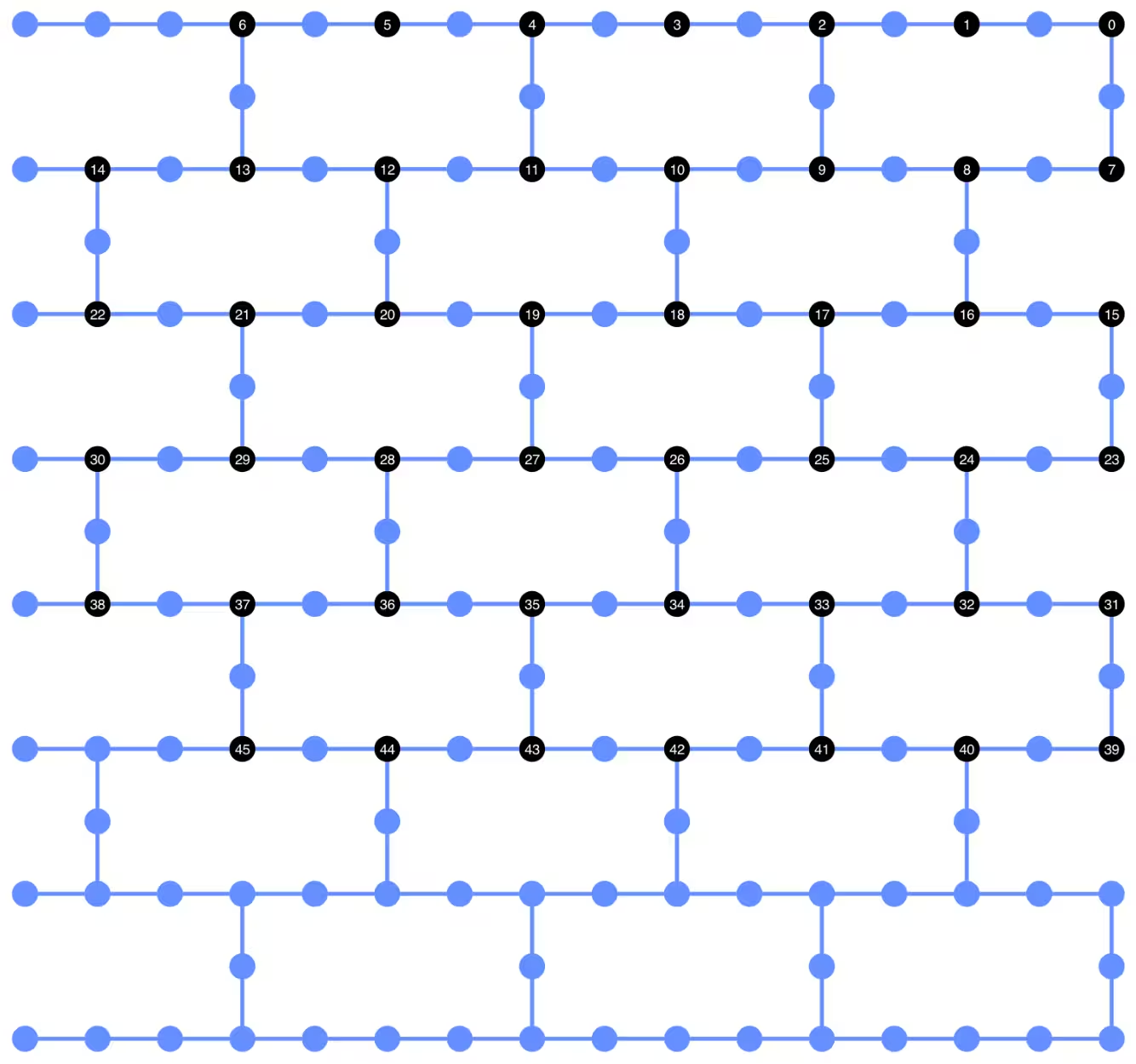
เราสามารถแสดง qubit layout ของ Circuit ที่ Transpile แล้วด้านล่างนี้ วงกลมสีดำแสดง data qubit และ ancilla qubit ที่ใช้ใน dynamic circuit implementation

def _heron_coords_r2():
    cord_map = np.array(
        [
            [
                0,
                1,
                2,
                3,
                4,
                5,
                6,
                7,
                8,
                9,
                10,
                11,
                12,
                13,
                14,
                15,
                3,
                7,
                11,
                15,
                0,
                1,
                2,
                3,
                4,
                5,
                6,
                7,
                8,
                9,
                10,
                11,
                12,
                13,
                14,
                15,
                1,
                5,
                9,
                13,
                0,
                1,
                2,
                3,
                4,
                5,
                6,
                7,
                8,
                9,
                10,
                11,
                12,
                13,
                14,
                15,
                3,
                7,
                11,
                15,
                0,
                1,
                2,
                3,
                4,
                5,
                6,
                7,
                8,
                9,
                10,
                11,
                12,
                13,
                14,
                15,
                1,
                5,
                9,
                13,
                0,
                1,
                2,
                3,
                4,
                5,
                6,
                7,
                8,
                9,
                10,
                11,
                12,
                13,
                14,
                15,
                3,
                7,
                11,
                15,
                0,
                1,
                2,
                3,
                4,
                5,
                6,
                7,
                8,
                9,
                10,
                11,
                12,
                13,
                14,
                15,
                1,
                5,
                9,
                13,
                0,
                1,
                2,
                3,
                4,
                5,
                6,
                7,
                8,
                9,
                10,
                11,
                12,
                13,
                14,
                15,
                3,
                7,
                11,
                15,
                0,
                1,
                2,
                3,
                4,
                5,
                6,
                7,
                8,
                9,
                10,
                11,
                12,
                13,
                14,
                15,
            ],
            -1
            * np.array([j for i in range(15) for j in [i] * [16, 4][i % 2]]),
        ],
        dtype=int,
    )

    hcords = []
    ycords = cord_map[0]
    xcords = cord_map[1]
    for i in range(156):
        hcords.append([xcords[i] + 1, np.abs(ycords[i]) + 1])

    return hcords

plot_circuit_layout(
    dynamic_isa_circuits_dd[8],
    backend,
    qubit_coordinates=_heron_coords_r2(),
    view="virtual",
)

หมายเหตุ

ถ้าเกิด error เกี่ยวกับ neato ที่ไม่พบจาก plot_circuit_layout() ให้ตรวจสอบว่าคุณติดตั้งแพ็กเกจ graphviz และมีให้ใช้งานใน PATH ของคุณแล้ว ถ้าติดตั้งไปในตำแหน่งที่ไม่ใช่ค่าเริ่มต้น (เช่น ใช้ homebrew บน MacOS) คุณอาจต้องอัปเดตตัวแปร environment PATH ของคุณ สิ่งนี้สามารถทำได้ภายใน notebook นี้โดยใช้คำสั่งดังนี้:

import os
os.environ['PATH'] = f"path/to/neato{os.pathsep}{os.environ['PATH']}"

dynamic_isa_circuits[1].draw(fold=-1, output="mpl", idle_wires=False)

dynamic_isa_circuits_dd[1].draw(fold=-1, output="mpl", idle_wires=False)

การ Transpile โดยใช้ MidCircuitMeasure

MidCircuitMeasure เป็นส่วนเพิ่มเติมของการดำเนินการวัดที่มีอยู่ ซึ่งถูก calibrate มาโดยเฉพาะเพื่อทำ mid-circuit measurements คำสั่ง MidCircuitMeasure จะ map ไปยังคำสั่ง measure_2 ที่ Backend รองรับ โปรดทราบว่า measure_2 ไม่ได้รองรับบน Backend ทุกตัว คุณสามารถใช้ service.backends(filters=lambda b: "measure_2" in b.supported_instructions) เพื่อหา Backend ที่รองรับ ที่นี่เราจะแสดงวิธี Transpile Circuit เพื่อให้ mid-circuit measurements ที่กำหนดไว้ใน Circuit ถูก execute โดยใช้การดำเนินการ MidCircuitMeasure หาก Backend รองรับ

ด้านล่าง เราจะพิมพ์ค่า duration สำหรับคำสั่ง measure_2 และคำสั่ง measure มาตรฐาน

print(
    f'Mid-circuit measurement `measure_2` duration: {backend.instruction_durations.get('measure_2',0) * backend.dt * 1e9/1e3} μs'
)
print(
    f'Terminal measurement `measure` duration: {backend.instruction_durations.get('measure',0) * backend.dt *1e9/1e3} μs'
)

Mid-circuit measurement `measure_2` duration:  1.624 μs
Terminal measurement `measure` duration: 2.2 μs

"""Pass that replaces terminal measures in the middle of the circuit with
MidCircuitMeasure instructions."""

class ConvertToMidCircuitMeasure(TransformationPass):
    """This pass replaces terminal measures in the middle of the circuit with
    MidCircuitMeasure instructions.
    """

    def __init__(self, target):
        super().__init__()
        self.target = target

    def run(self, dag):
        """Run the pass on a dag."""
        mid_circ_measure = None
        for inst in self.target.instructions:
            if isinstance(inst[0], Instruction) and inst[0].name.startswith(
                "measure_"
            ):
                mid_circ_measure = inst[0]
                break
        if not mid_circ_measure:
            return dag

        final_measure_nodes = calc_final_ops(dag, {"measure"})
        for node in dag.op_nodes(Measure):
            if node not in final_measure_nodes:
                dag.substitute_node(node, mid_circ_measure, inplace=True)

        return dag

pm = PassManager(ConvertToMidCircuitMeasure(backend.target))

dynamic_isa_circuits_meas2 = [pm.run(circ) for circ in dynamic_isa_circuits]
dynamic_pubs_meas2 = [(circ, params) for circ in dynamic_isa_circuits_meas2]

dynamic_isa_circuits_dd_meas2 = [
    pm.run(circ) for circ in dynamic_isa_circuits_dd
]
dynamic_pubs_dd_meas2 = [
    (circ, params) for circ in dynamic_isa_circuits_dd_meas2
]

การ Transpile สำหรับ unitary circuits

เพื่อให้การเปรียบเทียบระหว่าง dynamic circuits และ unitary circuit ที่เทียบเคียงกันเป็นธรรม เราจะใช้ชุด physical qubit เดียวกับที่ใช้ใน dynamic circuits สำหรับ data qubit เป็น layout ในการ Transpile unitary circuits

init_layout = [
    dynamic_layout[ind] for ind in range(circuits_unitary[0].num_qubits)
]

pm = generate_preset_pass_manager(
    target=backend.target,
    initial_layout=init_layout,
    optimization_level=3,
)

def transpile_minimize(circ: QuantumCircuit, pm: PassManager, iterations=10):
    """Transpile circuits for specified number of iterations and return the one with smallest two-qubit gate depth"""
    circs = [pm.run(circ) for i in range(iterations)]
    circs_sorted = sorted(
        circs,
        key=lambda x: x.depth(lambda x: x.operation.num_qubits == 2),
    )
    return circs_sorted[0]

unitary_isa_circuits = []
for circ in circuits_unitary:
    circ_t = transpile_minimize(circ, pm, iterations=100)
    unitary_isa_circuits.append(circ_t)

unitary_pubs = [(circ, params) for circ in unitary_isa_circuits]

เราแสดง qubit layout ของ unitary circuits ที่ Transpile แล้ว วงกลมสีดำระบุ physical qubit ที่ใช้ใน Transpile unitary circuits และ index ของมันสอดคล้องกับ virtual qubit index เมื่อเปรียบเทียบกับ layout ที่แสดงสำหรับ dynamic circuits เราสามารถยืนยันได้ว่า unitary circuits ใช้ชุด physical qubit เดียวกับ data qubit ใน dynamic circuits

plot_circuit_layout(
    unitary_isa_circuits[-1],
    backend,
    qubit_coordinates=_heron_coords_r2(),
    view="virtual",
)

ตอนนี้เราจะเพิ่ม DD sequence ให้กับ Circuit ที่ Transpile แล้ว และสร้าง PUBs ที่สอดคล้องกันสำหรับการส่ง job

pm_dd = PassManager(
    [
        ALAPScheduleAnalysis(target=backend.target),
        PadDynamicalDecoupling(
            dd_sequence=[
                XGate(),
                RZGate(np.pi),
                XGate(),
                RZGate(-np.pi),
            ],
            spacing=[1 / 4, 1 / 2, 0, 0, 1 / 4],
            target=backend.target,
        ),
    ]
)

unitary_isa_circuits_dd = pm_dd.run(unitary_isa_circuits)
unitary_pubs_dd = [(circ, params) for circ in unitary_isa_circuits_dd]

เปรียบเทียบ two-qubit gate depth ของ unitary และ dynamic circuits

# compare circuit depth of unitary and dynamic circuit implementations
unitary_depth = [
    unitary_isa_circuits[i].depth(lambda x: x.operation.num_qubits == 2)
    for i in range(len(unitary_isa_circuits))
]

dynamic_depth = [
    dynamic_isa_circuits[i].depth(lambda x: x.operation.num_qubits == 2)
    for i in range(len(dynamic_isa_circuits))
]

plt.plot(
    list(range(len(unitary_depth))),
    unitary_depth,
    label="unitary circuits",
    color="#be95ff",
)
plt.plot(
    list(range(len(dynamic_depth))),
    dynamic_depth,
    label="dynamic circuits",
    color="#ff7eb6",
)
plt.xlabel("Trotter steps")
plt.ylabel("Two-qubit depth")
plt.legend()

<matplotlib.legend.Legend at 0x374225760>

ข้อดีหลักของ measurement-based circuit คือ เมื่อ implement ZZ interactions หลายตัว CX layer สามารถทำงานแบบขนานได้ และการวัดสามารถเกิดขึ้นพร้อมกัน ทั้งนี้เพราะ ZZ interactions ทั้งหมด commute กัน ดังนั้นการคำนวณจึงสามารถทำได้ด้วย measurement depth 1 หลังจาก Transpile Circuit แล้ว เราสังเกตว่าวิธี dynamic circuit ให้ two-qubit depth ที่สั้นกว่าวิธี unitary มาตรฐานอย่างมีนัยสำคัญ โดยมีข้อแม้ว่า mid-circuit measurement เพิ่มเติมและ classical feedforward เองก็ใช้เวลาและนำเสนอแหล่งที่มาของความผิดพลาดในตัวเอง

ขั้นตอนที่ 3: รันด้วย Qiskit primitives

โหมดทดสอบในเครื่อง

ก่อนจะส่งงานไปรันบนฮาร์ดแวร์จริง เราสามารถทดสอบ dynamic circuit ด้วย simulation ขนาดเล็กผ่าน local testing mode

aer_sim = AerSimulator()
pm = generate_preset_pass_manager(backend=aer_sim, optimization_level=1)
circuit_dynamic_test.measure_all()
isa_qc = pm.run(circuit_dynamic_test)
with Batch(backend=aer_sim) as batch:
    sampler = Sampler(mode=batch)
    result = sampler.run([(isa_qc, params)]).result()

print(
    "Simulated average magnetization at trotter step = 1 at three theta values"
)
result[0].data["meas"].expectation_values(obs_dynamic_test[0])

Simulated average magnetization at trotter step = 1 at three theta values

array([ 0.16666667,  0.01855469, -0.13476562])

การ simulation แบบ MPS

สำหรับ Circuit ขนาดใหญ่ เราสามารถใช้ simulator แบบ matrix_product_state (MPS) ซึ่งให้ผลลัพธ์โดยประมาณของค่า expectation value ตาม bond dimension ที่เลือกไว้ ผลลัพธ์จากการ simulation ด้วย MPS จะถูกใช้เป็นเส้นฐาน (baseline) สำหรับเปรียบเทียบกับผลจากฮาร์ดแวร์ในภายหลัง

# The MPS simulation below took approximately 7 minutes to run on a laptop with Apple M1 chip

mps_backend = AerSimulator(
    method="matrix_product_state",
    matrix_product_state_truncation_threshold=1e-5,
    matrix_product_state_max_bond_dimension=100,
)
mps_sampler = Aer_Sampler.from_backend(mps_backend)

shots = 4096

data_sim = []
for j in range(points):
    circ_list = [
        circ.assign_parameters([params[j]]) for circ in circuits_unitary
    ]

    mps_job = mps_sampler.run(circ_list, shots=shots)
    result = mps_job.result()

    point_data = [
        result[d].data["meas"].expectation_values(observables_unitary)
        for d in depths
    ]

    data_sim.append(point_data)  # data at one theta value

data_sim = np.array(data_sim)

เมื่อเตรียม Circuit และ observables พร้อมแล้ว เราก็รัน Circuit เหล่านั้นบนฮาร์ดแวร์โดยใช้ Sampler primitive

ที่นี่เราจะส่งงานสามชุดสำหรับ unitary_pubs, dynamic_pubs และ dynamic_pubs_dd แต่ละชุดประกอบด้วย Circuit ที่มีพารามิเตอร์สำหรับ Trotter step เก้าขั้นตอนที่แตกต่างกัน โดยมีพารามิเตอร์ $\theta$ สามค่า

shots = 10000

with Batch(backend=backend) as batch:
    sampler = Sampler(mode=batch)

    sampler.options.experimental = {
        "execution": {
            "scheduler_timing": True
        },  # set to True to retrieve circuit timing info
    }

    job_unitary = sampler.run(unitary_pubs, shots=shots)
    print(f"unitary: {job_unitary.job_id()}")

    job_unitary_dd = sampler.run(unitary_pubs_dd, shots=shots)
    print(f"unitary_dd: {job_unitary_dd.job_id()}")

    job_dynamic = sampler.run(dynamic_pubs, shots=shots)
    print(f"dynamic: {job_dynamic.job_id()}")

    job_dynamic_dd = sampler.run(dynamic_pubs_dd, shots=shots)
    print(f"dynamic_dd: {job_dynamic_dd.job_id()}")

    job_dynamic_meas2 = sampler.run(dynamic_pubs_meas2, shots=shots)
    print(f"dynamic_meas2: {job_dynamic_meas2.job_id()}")

    job_dynamic_dd_meas2 = sampler.run(dynamic_pubs_dd_meas2, shots=shots)
    print(f"dynamic_dd_meas2: {job_dynamic_dd_meas2.job_id()}")

unitary: d5dtt0ldq8ts73fvbhj0
unitary: d5dtt11smlfc739onuag
dynamic: d5dtt1hsmlfc739onuc0
dynamic_dd: d5dtt25jngic73avdne0
dynamic_meas2: d5dtt2ldq8ts73fvbhm0
dynamic_dd_meas2: d5dtt2tjngic73avdnf0

ขั้นตอนที่ 4: ประมวลผลและส่งคืนผลลัพธ์ในรูปแบบ classical ที่ต้องการ

หลังจากงานเสร็จสิ้น เราสามารถดึงข้อมูลระยะเวลาของ Circuit จาก metadata ของผลลัพธ์งาน และแสดงภาพข้อมูล schedule ของ Circuit ได้ หากต้องการอ่านเพิ่มเติมเกี่ยวกับการแสดงภาพข้อมูล scheduling ของ Circuit ดูได้ที่ หน้านี้

# Circuit durations is reported in the unit of `dt` which can be retrieved from `Backend` object
unitary_durations = [
    job_unitary.result()[i].metadata["compilation"]["scheduler_timing"][
        "circuit_duration"
    ]
    for i in depths
]

dynamic_durations = [
    job_dynamic.result()[i].metadata["compilation"]["scheduler_timing"][
        "circuit_duration"
    ]
    for i in depths
]

dynamic_durations_meas2 = [
    job_dynamic_meas2.result()[i].metadata["compilation"]["scheduler_timing"][
        "circuit_duration"
    ]
    for i in depths
]

result_dd = job_dynamic_dd.result()[1]
circuit_schedule_dd = result_dd.metadata["compilation"]["scheduler_timing"][
    "timing"
]

# to visualize the circuit schedule, one can show the figure below
fig_dd = draw_circuit_schedule_timing(
    circuit_schedule=circuit_schedule_dd,
    included_channels=None,
    filter_readout_channels=False,
    filter_barriers=False,
    width=1000,
)

# Save to a file since the figure is large
fig_dd.write_html("scheduler_timing_dd.html")

เราวาดกราฟแสดงระยะเวลาของ Circuit สำหรับ unitary circuit และ dynamic circuit จากกราฟด้านล่าง เราจะเห็นว่าแม้จะมีเวลาที่ต้องใช้สำหรับการวัดกลางวงจร (mid-circuit measurement) และการดำเนินการ classical แต่การ implement dynamic circuit ด้วย measure_2 ให้ระยะเวลาของ Circuit ที่ใกล้เคียงกับการ implement แบบ unitary

# visualize circuit durations

def convert_dt_to_microseconds(circ_duration: List, backend_dt: float):
    dt = backend_dt * 1e6  # dt in microseconds
    return list(map(lambda x: x * dt, circ_duration))

dt = backend.target.dt
plt.plot(
    depths,
    convert_dt_to_microseconds(unitary_durations, dt),
    color="#be95ff",
    linestyle=":",
    label="unitary",
)
plt.plot(
    depths,
    convert_dt_to_microseconds(dynamic_durations, dt),
    color="#ff7eb6",
    linestyle="-.",
    label="dynamic",
)
plt.plot(
    depths,
    convert_dt_to_microseconds(dynamic_durations_meas2, dt),
    color="#ff7eb6",
    linestyle="-.",
    marker="s",
    mfc="none",
    label="dynamic w/ meas2",
)

plt.xlabel("Trotter steps")
plt.ylabel(r"Circuit durations in $\mu$s")
plt.legend()

<matplotlib.legend.Legend at 0x17f73c6e0>

หลังจากงานเสร็จสิ้น เราดึงข้อมูลด้านล่างและคำนวณค่าแมกนีไทเซชันเฉลี่ยที่ประมาณโดย observables observables_unitary หรือ observables_dynamic ที่เราสร้างขึ้นก่อนหน้า

runs = {
    "unitary": (
        job_unitary,
        [observables_unitary] * len(circuits_unitary),
    ),
    "unitary_dd": (
        job_unitary_dd,
        [observables_unitary] * len(circuits_unitary),
    ),
    # Omitting Dyn w/o DD and Dynamic w/ DD plots for better readability
    # "dynamic": (job_dynamic, observables_dynamic),
    # "dynamic_dd": (job_dynamic_dd, observables_dynamic),
    "dynamic_meas2": (job_dynamic_meas2, observables_dynamic),
    "dynamic_dd_meas2": (
        job_dynamic_dd_meas2,
        observables_dynamic,
    ),
}

data_dict = {}
for key, (job, obs) in runs.items():
    data = []
    for i in range(points):
        data.append(
            [
                job.result()[ind].data["meas"].expectation_values(obs[ind])[i]
                for ind in depths
            ]
        )
    data_dict[key] = data

ด้านล่างเราวาดกราฟแสดงค่าแมกนีไทเซชันของสปินเป็นฟังก์ชันของ Trotter step ที่ค่า $\theta$ ต่างกัน ซึ่งสอดคล้องกับความเข้มของสนามแม่เหล็กในเครื่องที่แตกต่างกัน เราวาดกราฟทั้งผลลัพธ์จากการ simulation ด้วย MPS สำหรับ unitary ideal circuit ที่คำนวณไว้ล่วงหน้า พร้อมกับผลลัพธ์จากการทดลองจาก:

1. การรัน unitary circuit ด้วย DD
2. การรัน dynamic circuit ด้วย DD และ MidCircuitMeasure

plt.figure(figsize=(10, 6))

colors = ["#0f62fe", "#be95ff", "#ff7eb6"]
for i in range(points):
    plt.plot(
        depths,
        data_sim[i],
        color=colors[i],
        linestyle="solid",
        label=f"θ={pi_check(i*max_angle/(points-1))} (MPS)",
    )
    # plt.plot(
    #     depths,
    #     data_dict["unitary"][i],
    #     color=colors[i],
    #     linestyle=":",
    #     label=f"θ={pi_check(i*max_angle/(points-1))} (Unitary)",
    # )

    plt.plot(
        depths,
        data_dict["unitary_dd"][i],
        color=colors[i],
        marker="o",
        mfc="none",
        linestyle=":",
        label=f"θ={pi_check(i*max_angle/(points-1))} (Unitary w/DD)",
    )

    # Omitting Dyn w/o DD and Dynamic w/ DD plots for better readability
    # plt.plot(
    #     depths,
    #     data_dict["dynamic"][i],
    #     color=colors[i],
    #     linestyle="-.",
    #     label=f"θ={pi_check(i*max_angle/(points-1))} (Dyn w/o DD)",
    # )
    # plt.plot(
    #     depths,
    #     data_dict["dynamic_dd"][i],
    #     marker="D",
    #     mfc="none",
    #     color=colors[i],
    #     linestyle="-.",
    #     label=f"θ={pi_check(i*max_angle/(points-1))} (Dynamic w/ DD)",
    # )

    # plt.plot(
    #     depths,
    #     data_dict["dynamic_meas2"][i],
    #     color=colors[i],
    #     marker="s",
    #     mfc="none",
    #     linestyle=':',
    #     label=f"θ={pi_check(i*max_angle/(points-1))} (Dynamic w/ MidCircuitMeas)",
    # )

    plt.plot(
        depths,
        data_dict["dynamic_dd_meas2"][i],
        color=colors[i],
        marker="*",
        markersize=8,
        linestyle=":",
        label=f"θ={pi_check(i*max_angle/(points-1))} (Dynamic w/ DD & MidCircuitMeas)",
    )

plt.xlabel("Trotter steps", fontsize=16)
plt.ylabel("Average magnetization", fontsize=16)
plt.xticks(rotation=45)
handles, labels = plt.gca().get_legend_handles_labels()
plt.legend(
    handles,
    labels,
    loc="upper right",
    bbox_to_anchor=(1.46, 1.0),
    shadow=True,
    ncol=1,
)
plt.title(
    f"{hex_rows}x{hex_cols} hex ring, {num_qubits} data qubits, {len(ancilla)} ancilla qubits \n{backend.name}: Sampler"
)
plt.show()

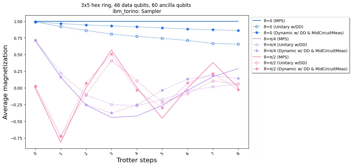
เมื่อเปรียบเทียบผลลัพธ์จากการทดลองกับการ simulation เราเห็นว่าการ implement dynamic circuit (เส้นประพร้อมดาว) โดยรวมมีประสิทธิภาพดีกว่าการ implement unitary มาตรฐาน (เส้นประพร้อมวงกลม) โดยสรุป เราได้นำเสนอ dynamic circuit ในฐานะวิธีแก้ปัญหาสำหรับการ simulate โมเดล Ising spin บนโครงตาข่ายรังผึ้ง (honeycomb lattice) ซึ่งเป็นโทโพโลยีที่ไม่ได้เป็นแบบ native ของฮาร์ดแวร์ วิธีการ dynamic circuit ช่วยให้เกิดปฏิสัมพันธ์ ZZ ระหว่าง Qubit ที่ไม่ได้อยู่ใกล้กัน โดยมีความลึกของ Gate สองQubit ที่สั้นกว่าการใช้ SWAP Gate แลกกับการต้องใช้ ancilla Qubit เพิ่มเติมและการดำเนินการ classical feedforward

อ้างอิง

[1] Quantum computing with Qiskit, by Javadi-Abhari, A., Treinish, M., Krsulich, K., Wood, C.J., Lishman, J., Gacon, J., Martiel, S., Nation, P.D., Bishop, L.S., Cross, A.W. and Johnson, B.R., 2024. arXiv preprint arXiv:2405.08810 (2024)