การสังเกตพลศาสตร์แฮดรอนแบบไม่เอเบเลียนที่แข็งแกร่งและมีความอาพันธ์บนโปรเซสเซอร์ควอนตัมที่มีสัญญาณรบกวน
ประมาณการใช้งาน: 6 นาทีบนโปรเซสเซอร์ Heron (ibm_boston หรือเทียบเท่า) (หมายเหตุ: นี่เป็นเพียงการประมาณการเท่านั้น ระยะเวลารันจริงของคุณอาจแตกต่างออกไป)
ผลลัพธ์การเรียนรู้
-
ทฤษฎีเกจแลตทิซแบบไม่เอเบเลียน (โดยเฉพาะ SU(2)) สามารถถูกจัดรูปแบบใหม่โดยใช้กรอบงาน Loop-String-Hadron (LSH) เพื่อการจำลองควอนตัมที่มีประสิทธิภาพได้อย่างไร
-
วิธีสร้างวงจรวิวัฒนาการเวลาแบบ Trotterized สำหรับ Hamiltonian ของทฤษฎีเกจ SU(2) โดยประมาณ และแมปมันลงบนคิวบิต
-
วิธีรันวงจรเหล่านี้บนฮาร์ดแวร์ IBM Quantum® โดยใช้ Qiskit Estimator primitive พร้อมการลดข้อผิดพลาดในการอ่านค่า (readout error mitigation)
ข้อกำหนดเบื้องต้น
-
ความคุ้นเคยพื้นฐานกับแนวคิดทฤษฎีสนามควอนตัม (มีประโยชน์แต่ไม่จำเป็น ส่วนพื้นฐานจะครอบคลุมสิ่งจำเป็น)
ความเป็นมา
แรงจูงใจ
Quantum Chromodynamics (QCD) ทฤษฎีเกจ SU(3) ของแรงนิวเคลียร์อย่างเข้ม ยึดเหนี่ยวควาร์กเข้าด้วยกันเป็นแฮดรอนและควบคุมการกักขัง (confinement) และการแตกของสาย (string breaking) วิธีการแลตทิซ QCD แบบคลาสสิกทำงานได้ดีกับคุณสมบัติแบบสถิต แต่ไม่สามารถจำลองพลศาสตร์แบบเวลาจริงได้เนื่องจากปัญหาเครื่องหมาย (sign problem) คอมพิวเตอร์ควอนตัมนำเสนอเส้นทางในการหลีกเลี่ยงอุปสรรคนี้โดยการเข้ารหัสองศาความอิสระของสนามเกจโดยตรงลงบนคิวบิต
บทเรียนนี้สาธิตการจำลองดังกล่าว: ใช้ฮาร์ดแวร์ IBM Quantum เพื่อจำลองการแพร่กระจายแฮดรอนแบบเวลาจริงในทฤษฎีเกจแลตทิซ SU(2) แบบ (1+1)-มิติ — ทฤษฎีเกจแบบไม่เอเบเลียนที่ง่ายที่สุดและเป็นก้าวสำคัญสู่ QCD เต็มรูปแบบ
Kogut-Susskind Hamiltonian
ทฤษฎีนี้ถูกกำหนดขึ้นบนแลตทิซเชิงพื้นที่หนึ่งมิติที่มีเฟอร์มิออนแบบสแตกเกอร์ (matter) อยู่บนไซต์ และสนามเกจ SU(2) อยู่บนลิงก์ หลังจากปรับสเกลให้ไม่มีมิติ Hamiltonian คือ:
โดยที่ คือพลังงานสนามโครโมอิเล็กทริก คือเทอมมวลแบบสแตกเกอร์ คือเทอมปฏิสัมพันธ์แมทเทอร์-เกจ (การกระโดด/hopping) เข้ารหัสมวลเฟอร์มิออน และ คือความแรงของปฏิสัมพันธ์ ลิมิตต่อเนื่อง (continuum limit) ของทฤษฎีนี้อยู่ที่ และ
กรอบงาน Loop-String-Hadron (LSH)
ความท้าทายสำคัญคือปริภูมิฮิลเบิร์ตของสนามเกจบนแต่ละลิงก์มีมิติไม่จำกัด กรอบงาน Loop-String-Hadron (LSH) จัดการกับสิ่งนี้โดยการจัดรูปแบบทฤษฎีใหม่ในรูปของตัวแปรที่ไม่แปรเปลี่ยนต่อเกจ (gauge-invariant) — ลูปฟลักซ์ สายที่เชื่อมประจุที่แยกจากกัน และแฮดรอน (คู่เฟอร์มิออนแบบเกจซิงเกลตที่ไซต์) ในฐาน LSH กฎของ Gauss จะเป็นจริงโดยอัตโนมัติจากโครงสร้าง ดังนั้นสถานะฐานทุกตัวจึงเป็นสถานะทางฟิสิกส์ แต่ละไซต์แลตทิซถูกกำหนดลักษณะด้วยเลขควอนตัมสามตัว ซึ่งแทนจำนวนลูป สายขาเข้า และสายขาออก โดยที่ เป็นแบบเฟอร์มิออน และ เป็นแบบโบซอน จำนวนเฟอร์มิออนท้องถิ่นถูกกำหนดจากสิ่งเหล่านี้เป็น สำหรับไซต์เลขคู่ และ สำหรับไซต์เลขคี่
จาก Hamiltonian เต็มรูปแบบสู่วงจรควอนตัม: การประมาณค่าสำคัญสามประการ
วงจรควอนตัมไม่ได้จำลอง Hamiltonian SU(2) เต็มรูปแบบอย่างแม่นยำ แต่จะนำการประมาณค่าแบบควบคุมชุดหนึ่งไปใช้ ซึ่งใช้ได้ผลในระบบการคู่ควบแบบอ่อน (weak-coupling regime) () การเข้าใจว่าอะไรถูกประมาณและอะไรไม่ถูกประมาณเป็นสิ่งจำเป็น:
การประมาณค่า 1 — ลิมิตการคู่ควบแบบอ่อนสำหรับ : Hamiltonian ปฏิสัมพันธ์เต็มรูปแบบ (สมการที่ 16 ใน [1]) มีค่าสัมประสิทธิ์นำหน้าที่ขึ้นกับเลขควอนตัมโบซอน ผ่านเทอมเช่น ในระบบการคู่ควบแบบอ่อน () พลศาสตร์ถูกครอบงำโดยเทอมไฟฟ้า ซึ่งเอื้อต่อสถานะที่มี มาก สำหรับ อัตราส่วน และค่าสัมประสิทธิ์นำหน้าเหล่านี้ทั้งหมดจะลดรูปเป็นหนึ่ง Hamiltonian ปฏิสัมพันธ์จึงลดรูปลงเหลือเพียงการกระโดดระหว่างเพื่อนบ้านที่ใกล้ที่สุดแบบท้องถิ่นล้วนๆ:
ซึ่งไม่ขึ้นกับ และกระทำเฉพาะกับคิวบิตเฟอร์มิออน เท่านั้น
การประมาณค่า 2 — ฟลักซ์เฉลี่ยแบบทั่วโลกสำหรับ : พลังงานไฟฟ้าขึ้นกับ ที่แต่ละลิงก์ ในสุญญากาศแบบคู่ควบอ่อน มีค่ามากและมีความสม่ำเสมอโดยประมาณ แทนที่ค่า ที่ขึ้นกับไซต์ด้วยค่าเฉลี่ยทั่วโลกค่าเดียว ทำให้ เป็นเฟสแนวทแยงที่เป็นสัดส่วนกับการจัดรูปเฟอร์มิออนที่แต่ละไซต์:
โดยที่ คือผลรวมบนไซต์ที่อยู่ในคอนฟิกูเรชันเฟอร์มิออน และ คือเฟสทั่วโลกที่คุณสามารถละเลยได้
การประมาณค่า 3 — Trotterization: ตัวดำเนินการวิวัฒนาการเวลาสำหรับขั้นตอนที่มีระยะเวลา ถูกแยกส่วนเป็น:
โดยที่ , และ การแยกส่วน Trotter ลำดับที่หนึ่งนี้ก่อให้เกิดความคลาดเคลื่อนที่หายไปเมื่อ เรากำหนด ตลอดทั้งบทเรียน
ผลลัพธ์ของการประมาณค่าสามประการนี้คือ มีเพียงคิวบิตเฟอร์มิออนสองตัวต่อไซต์ เท่านั้นที่มีพลศาสตร์ — องศาความอิสระของโบซอน ถูกดูดซับเข้าไปในพารามิเตอร์ที่มีประสิทธิผลแล้ว สิ่งนี้ให้วงจรที่กะทัดรัดด้วยคิวบิต ตัวสำหรับไซต์แลตทิซ ไซต์ โดยที่แต่ละขั้น Trotter มีความลึกของเกตสองคิวบิตคงที่ (13 ต่อขั้น)
บทเรียนนี้จำลองอะไร
บทเรียนนี้จำลองการแพร่กระจายแฮดรอน: เริ่มต้นจากสุญญากาศแบบคู่ควบแรง (สถานะผลคูณ) วางมีซอนไว้ที่ศูนย์กลางของแลตทิซ และให้วิวัฒนาการตามเวลา โปรโตคอลการวัดเชิงผลต่าง — รันวงจรทั้งแบบมีและไม่มีมีซอนตรงกลาง แล้วลบออก — แยกสัญญาณแฮดรอนที่สอดคล้องกันออกจากทั้งสัญญาณรบกวนฮาร์ดแวร์และผลกระทบจากขอบเขต ผลลัพธ์คือรูปแบบกรวยแสง (light-cone) ของการแกว่งความหนาแน่นเฟอร์มิออนที่เป็นลักษณะเฉพาะของโหมดการหายใจของมีซอนที่ถูกกักขัง
ข้อกำหนด
ก่อนเริ่มบทเรียนนี้ ให้ติดตั้งสิ่งต่อไปนี้:
-
Qiskit SDK v2.0 หรือใหม่กว่า พร้อมการรองรับ visualization
-
Qiskit Runtime v0.22 หรือใหม่กว่า (
pip install qiskit-ibm-runtime) -
แพ็กเกจ Pauli Propagation (
pip install pauli-prop) -
NumPy (
pip install numpy) -
Matplotlib (
pip install matplotlib)
การตั้งค่า
เริ่มต้นด้วยการนำเข้าไลบรารีที่จำเป็นและกำหนดฟังก์ชันตัวช่วยที่สร้างวงจรควอนตัมสำหรับวิวัฒนาการเวลาแบบ LSH มีฟังก์ชันสร้างวงจรหลักสามตัว:
-
pair_hamiltonian_circuit: นำยูนิทารีสองคิวบิต ไปใช้สำหรับ Hamiltonian ปฏิสัมพันธ์โดยประมาณระหว่างไซต์ที่อยู่ติดกัน การแยกส่วนเกตคือ: -
electric_hamiltonian_circuit: นำยูนิทารีสองคิวบิต ไปใช้สำหรับพลังงานสนามไฟฟ้าโดยประมาณที่แต่ละไซต์ การแยกส่วนเกตคือ: -
construct_circuit: ประกอบวงจร Trotterized เต็มรูปแบบ โดยเรียงชั้นเทอมปฏิสัมพันธ์ ไฟฟ้า และมวล พร้อมด้วยเกต SWAP เพื่อจัดการการเชื่อมต่อของคิวบิต
# Added by doQumentation — required packages for this notebook
!pip install -q matplotlib numpy pauli-prop qiskit qiskit-ibm-runtime
# Import libraries

import numpy as np
import matplotlib.pyplot as plt
from matplotlib.colors import TwoSlopeNorm
from qiskit.circuit import QuantumCircuit
from qiskit.quantum_info import SparsePauliOp
from typing import Optional

import warnings

warnings.filterwarnings("ignore")
def pair_hamiltonian_circuit(c: float) -> QuantumCircuit:
    """Two-qubit unitary for the approximate interaction Hamiltonian H_I.

    Implements exp(-i * c * H_I^approx) for one pair of neighboring sites,
    where c = delta_tau * x.
    """
    qc_temp = QuantumCircuit(2)
    qc_temp.cx(1, 0)
    qc_temp.h(1)
    qc_temp.rz(-c, 1)
    qc_temp.cx(0, 1)
    qc_temp.rz(c, 1)
    qc_temp.cx(0, 1)
    qc_temp.h(1)
    qc_temp.cx(1, 0)
    return qc_temp

def electric_hamiltonian_circuit(theta: float) -> QuantumCircuit:
    """Two-qubit unitary for the approximate electric field Hamiltonian H_E.

    Implements exp(-i * theta * H_E^approx) for one lattice site,
    where theta = -delta_tau * (n_bar_l / 2 + 3/4).
    """
    qc_temp = QuantumCircuit(2)
    qc_temp.x(0)
    qc_temp.rz(theta / 2, 0)
    qc_temp.cx(0, 1)
    qc_temp.rz(-theta / 2, 1)
    qc_temp.cx(0, 1)
    qc_temp.rz(theta / 2, 1)
    qc_temp.x(0)
    return qc_temp

def construct_circuit(
    num_lattice_point: int,
    num_trotter_steps: int,
    c: float,
    theta: float,
    m: float,
    theory: Optional[int] = 2,
    barriers: Optional[bool] = False,
    measurement: Optional[bool] = False,
    add_init_state: Optional[bool] = True,
    inverse_mid: Optional[bool] = False,
) -> QuantumCircuit:
    """Construct the full Trotterized time-evolution circuit.

    Builds a circuit implementing n Trotter steps of the approximate SU(2)
    LSH Hamiltonian evolution. The qubit layout uses a zigzag ordering:
    n_i(0), n_i(1), n_o(0), n_o(1), n_i(2), n_i(3), n_o(2), n_o(3), ...
    which minimizes the number of SWAP layers needed.

    Args:
        num_lattice_point: Number of lattice sites
        (num_qubits = 2 * num_lattice_point).
        num_trotter_steps: Number of Trotter steps.
        c: Interaction parameter (delta_tau * x).
        theta: Electric field phase parameter.
        m: Mass parameter (m_tilde = delta_tau * mu).
        theory: 1 for single chain, 2 for SU(2). Default 2.
        barriers: Insert barriers between Trotter layers for
        visualization.
        measurement: Append measurements at the end.
        add_init_state: Prepare the half-filled (strong-coupling vacuum)
        initial state.
        inverse_mid: Swap the central sites
        (for differential measurement protocol).
    """
    num_qubits = theory * num_lattice_point
    qc = QuantumCircuit(num_qubits)

    if num_trotter_steps <= 0:
        return qc

    # --- Initial state preparation ---
    if add_init_state:
        i = 1
        while i < num_lattice_point:
            for j in range(theory):
                qc.x(i + j * num_lattice_point)
            i = i + 2
        if inverse_mid:
            mid_lattice_qubits = [num_qubits // 2 - 1, num_qubits // 2]
            qc.x(mid_lattice_qubits)
    else:
        i = 1
        while i < num_qubits - 1:
            qc.swap(i, i + 1)
            i = i + 4

    # --- Trotter steps ---
    for step in range(num_trotter_steps):
        if barriers:
            qc.barrier()

        # First SWAP layer (skipped at step 0 — absorbed into initial state mapping)
        if step > 0:
            i = 1
            while i < num_qubits - 1:
                qc.swap(i, i + 1)
                i = i + 4

        # First layer of pair interactions
        j = 0
        while j < num_qubits - 2:
            circ = pair_hamiltonian_circuit(c)
            qc.compose(circ, [j, j + 1], inplace=True)
            j = j + 2
        if num_lattice_point % 2 == 0:
            circ = pair_hamiltonian_circuit(c)
            qc.compose(circ, [j, j + 1], inplace=True)

        # Second SWAP layer
        i = 1
        while i < num_qubits - 1:
            qc.swap(i, i + 1)
            i = i + theory

        # Second layer of pair interactions
        j = 2
        while j < num_qubits - 3:
            circ = pair_hamiltonian_circuit(c)
            qc.compose(circ, [j, j + 1], inplace=True)
            j = j + 2
        if num_lattice_point % 2 != 0:
            circ = pair_hamiltonian_circuit(c)
            qc.compose(circ, [j, j + 1], inplace=True)

        # Third SWAP layer
        i = 3
        while i < num_qubits - 1:
            qc.swap(i, i + 1)
            i = i + 2 * theory

        # Electric field term
        if theta != 0:
            e_circ = electric_hamiltonian_circuit(theta)
            for j in range(num_lattice_point):
                qc.compose(e_circ, [2 * j, 2 * j + 1], inplace=True)

        # Mass term: Rz(-m_tilde) for even sites, Rz(m_tilde) for odd sites
        for q in range(num_qubits):
            if q % 2 == 0:
                qc.rz(-1 * m, q)
            else:
                qc.rz(m, q)

    if measurement:
        qc.measure_all()

    return qc
def get_probabilities(expval: float):
    """Convert a Z-expectation value to site occupation probability.

    Since <Z> = p(0) - p(1), the occupation probability is p(1) = (1 - <Z>) / 2.
    """
    p1 = round((1 - expval) / 2, 3)
    return p1

def get_number(expval_data, num_lattice_point):
    """Convert raw Z-expectation values to staggered fermion number n_f at each site.

    n_f(r) = n_i(r) + n_o(r)           for even r
    n_f(r) = 2 - [n_i(r) + n_o(r)]     for odd r

    The two qubits per site encode (n_i, n_o), and occupation probabilities
    give us <n_i> and <n_o>.
    """
    N = []
    for expvals in expval_data:
        Pstep = [get_probabilities(expval) for expval in expvals]
        Nstep = []
        for k in range(num_lattice_point):
            val = Pstep[2 * k] + Pstep[2 * k + 1]
            a = 2 * (k % 2) + (1 - 2 * (k % 2)) * val
            Nstep.append(float(a))
        N.append(Nstep)
    return N

def calculate_difference(N, N_mid, num_lattice_point):
    """Differential measurement protocol: |n_f(meson) - n_f(vacuum)|.

    Subtracting the vacuum (SCV) evolution from the meson evolution
    isolates the coherent hadron signal from symmetric noise and boundary effects.
    """
    N_diff = []
    for i in range(len(N)):
        Nstep_diff = []
        for j in range(num_lattice_point):
            Nstep_diff.append(abs(N[i][j] - N_mid[i][j]))
        N_diff.append(Nstep_diff)
    return N_diff
ตัวอย่างตัวจำลองขนาดเล็ก
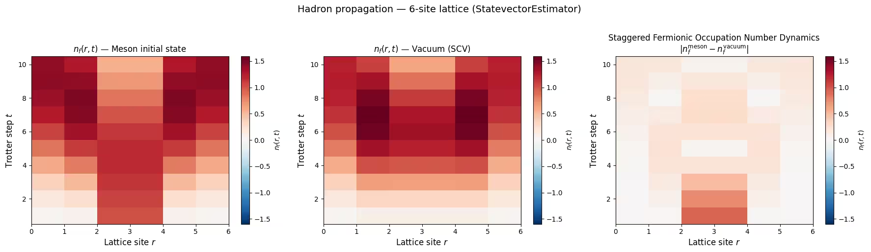
ก่อนอื่น มาสาธิต workflow ในระดับเล็กโดยใช้แลตทิซหกไซต์ (12 qubit) เพื่อให้คุณสามารถตรวจสอบการสร้าง Circuit และเข้าใจ observable ทางฟิสิกส์ก่อนที่จะรันบนฮาร์ดแวร์จริง
ขั้นตอนที่ 1: แมปข้อมูลนำเข้าแบบคลาสสิกไปยังปัญหาควอนตัม
กำหนดพารามิเตอร์ทางฟิสิกส์ที่ตรงกับ weak-coupling regime ที่ศึกษาในเปเปอร์ (, ) พารามิเตอร์ของ Circuit ที่ได้จากการคำนวณคือ:
-
(พารามิเตอร์ปฏิสัมพันธ์)
-
(เฟสของสนามไฟฟ้า)
-
(พารามิเตอร์มวล)
สำหรับแต่ละจำนวนขั้นตอน Trotter ให้สร้าง สอง Circuit: หนึ่งสำหรับการเตรียมมีซอนไว้ที่ตำแหน่งกึ่งกลาง (inverse_mid=True) และอีกหนึ่งสำหรับการเตรียมสุญญากาศแบบคู่ควบแรง (inverse_mid=False) โปรโตคอลการวัดแบบผลต่างจะลบการวิวัฒนาการของสุญญากาศออกเพื่อแยกสัญญาณของแฮดรอน
# Physical / circuit parameters
num_lattice_point = 6  # 6 lattice sites -> 12 qubits for SU(2)
num_qubits = 2 * num_lattice_point
c = 0.15  # delta_tau * x
theta = 0.01  # electric field phase
m = 0.03  # m_tilde = delta_tau * mu
trotter_steps = range(1, 11)  # 10 Trotter steps

print(f"Lattice sites: {num_lattice_point}, Qubits: {num_qubits}")
print(f"Parameters: c={c}, theta={theta}, m_tilde={m}")
Lattice sites: 6, Qubits: 12
Parameters: c=0.15, theta=0.01, m_tilde=0.03
# Build circuits: meson initial state and vacuum (SCV) initial state
circuits_mid = [
    construct_circuit(
        num_lattice_point,
        d,
        c,
        theta,
        m,
        barriers=False,
        measurement=False,
        add_init_state=True,
        inverse_mid=True,
    )
    for d in trotter_steps
]

circuits = [
    construct_circuit(
        num_lattice_point,
        d,
        c,
        theta,
        m,
        barriers=False,
        measurement=False,
        add_init_state=True,
        inverse_mid=False,
    )
    for d in trotter_steps
]

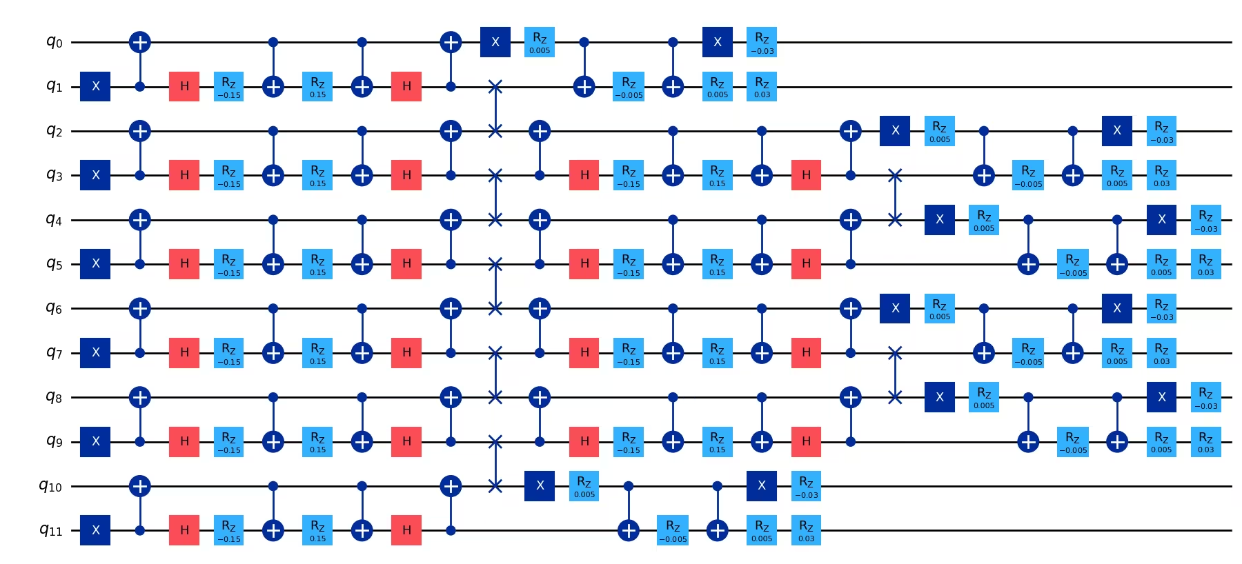
# Visualize a single Trotter step
print(
    f"Circuit for 1 Trotter step: {circuits[0].num_qubits} qubits, depth {circuits[0].depth()}"
)
circuits[0].draw("mpl", fold=-1)
Circuit for 1 Trotter step: 12 qubits, depth 26
ขั้นตอนที่ 2: ปรับปรุงปัญหาให้เหมาะกับการรันบนฮาร์ดแวร์ควอนตัม
กำหนด observable: การวัด แบบ single-qubit บน qubit ทุกตัว จาก คุณสามารถหาความน่าจะเป็นของการครอบครอง (occupation probability) และจากนั้นหาจำนวน staggered fermion ที่ตำแหน่งแลตทิซแต่ละแห่ง
# Z observable on each qubit
observables = [
    SparsePauliOp("I" * i + "Z" + "I" * (num_qubits - i - 1))
    for i in range(num_qubits)
]

print(f"Number of observables: {len(observables)}")
Number of observables: 12
ขั้นตอนที่ 3: รันโดยใช้ Qiskit primitive
ใช้ StatevectorEstimator สำหรับการจำลองแบบไม่มีสัญญาณรบกวนที่แม่นยำในระดับเล็ก
from qiskit.primitives import StatevectorEstimator

estimator = StatevectorEstimator()

# Run meson circuits
pubs_mid = [(circuit, observables) for circuit in circuits_mid]
result_mid = estimator.run(pubs_mid).result()

# Run vacuum (SCV) circuits
pubs = [(circuit, observables) for circuit in circuits]
result = estimator.run(pubs).result()

# Extract expectation values
raw_expvals_mid = [
    result_mid[i].data.evs[::-1] for i in range(len(circuits_mid))
]
raw_expvals = [result[i].data.evs[::-1] for i in range(len(circuits))]

print(f"Computed expectation values for {len(raw_expvals)} Trotter steps")
Computed expectation values for 10 Trotter steps
ขั้นตอนที่ 4: ประมวลผลภายหลังและคืนผลลัพธ์ในรูปแบบคลาสสิกที่ต้องการ
แปลงค่าคาดหวังเป็นจำนวน staggered fermion และใช้โปรโตคอลการวัดแบบผลต่าง (มีซอน สุญญากาศ) เพื่อสร้าง heatmap การแพร่กระจายของแฮดรอน ซึ่งจะสร้างโครงสร้างของ Figure 3 จากเปเปอร์อ้างอิงขึ้นมาใหม่: ตำแหน่งแลตทิซ บนแกน x, ขั้นตอน Trotter (เวลา) บนแกน y และ เป็นสเกลสี
# Compute fermion numbers
N_mid_sim = get_number(raw_expvals_mid, num_lattice_point)
N_sim = get_number(raw_expvals, num_lattice_point)
N_diff_sim = calculate_difference(N_mid_sim, N_sim, num_lattice_point)

# --- Reproduce Figure 3 style: Staggered Fermionic Occupation Number Dynamics ---
fig, axes = plt.subplots(1, 3, figsize=(18, 5))

# Convert to numpy arrays for plotting
N_mid_arr = np.array(N_mid_sim)
N_arr = np.array(N_sim)
N_diff_arr = np.array(N_diff_sim)

# Color scheme
vmax = max(max(sublist) for sublist in N_arr)
vmin = -vmax

# Meson evolution
norm1 = TwoSlopeNorm(vmin=vmin, vcenter=0, vmax=vmax)
im0 = axes[0].imshow(
    N_mid_arr,
    aspect="auto",
    origin="lower",
    cmap="RdBu_r",
    norm=norm1,
    extent=[0, num_lattice_point, 0.5, len(trotter_steps) + 0.5],
)
axes[0].set_xlabel("Lattice site $r$", fontsize=12)
axes[0].set_ylabel("Trotter step $t$", fontsize=12)
axes[0].set_title("$n_f(r,t)$ — Meson initial state", fontsize=12)
plt.colorbar(im0, ax=axes[0], label="$n_f(r,t)$")

# Vacuum (SCV) evolution
im1 = axes[1].imshow(
    N_arr,
    aspect="auto",
    origin="lower",
    cmap="RdBu_r",
    norm=norm1,
    extent=[0, num_lattice_point, 0.5, len(trotter_steps) + 0.5],
)
axes[1].set_xlabel("Lattice site $r$", fontsize=12)
axes[1].set_ylabel("Trotter step $t$", fontsize=12)
axes[1].set_title("$n_f(r,t)$ — Vacuum (SCV)", fontsize=12)
plt.colorbar(im1, ax=axes[1], label="$n_f(r,t)$")

# Differential: meson - vacuum
norm2 = TwoSlopeNorm(vmin=vmin, vcenter=0, vmax=vmax)
im2 = axes[2].imshow(
    N_diff_arr,
    aspect="auto",
    origin="lower",
    cmap="RdBu_r",
    norm=norm2,
    extent=[0, num_lattice_point, 0.5, len(trotter_steps) + 0.5],
)
axes[2].set_xlabel("Lattice site $r$", fontsize=12)
axes[2].set_ylabel("Trotter step $t$", fontsize=12)
axes[2].set_title(
    "Staggered Fermionic Occupation Number Dynamics\n$|n_f^{\\mathrm{meson}} - n_f^{\\mathrm{vacuum}}|$",
    fontsize=12,
)
plt.colorbar(im2, ax=axes[2], label="$n_f(r,t)$")

plt.suptitle(
    f"Hadron propagation — {num_lattice_point}-site lattice (StatevectorEstimator)",
    fontsize=14,
    y=1.02,
)
plt.tight_layout()
plt.show()
ตัวอย่างฮาร์ดแวร์ขนาดใหญ่
ตอนนี้เราจะขยายขนาดไปยังแลตทิซ 30 ไซต์ (60 qubit) บนฮาร์ดแวร์ IBM Quantum ในระดับนี้ Circuit ที่ 10 ขั้นตอน Trotter ประกอบด้วย two-qubit gate มากกว่า 3400 ตัว และ single-qubit gate 14,000 ตัว
ขั้นตอนที่ 1-4 (บีบอัดลงในโค้ดบล็อกเดียว)
แง่มุมสำคัญของ workflow บนฮาร์ดแวร์:
-
10 ขั้นตอน Trotter สำหรับ Circuit ของมีซอนและสุญญากาศ (สลับกันเพื่อลด drift ให้น้อยที่สุด)
-
การ transpile ด้วย
optimization_level=1— layout ของ Circuit นั้น isomorphic กับ topology ของอุปกรณ์อยู่แล้ว (chain เชิงเส้น) จึงไม่จำเป็นต้องมี routing SWAP Transpiler ถูกใช้เพียงเพื่อเลือก chain ของ physical qubit ที่มี noise ต่ำ และแยกสลาย gate ให้อยู่ใน native gate set -
EstimatorV2พร้อมการลด error ในการอ่านค่าแบบ TREX และ Pauli twirling -
Session แบบ
Batchเพื่อส่ง job ทั้งหมดพร้อมกัน
# -------------------------Step 1: Define parameters & build circuits-------------------------

from qiskit_ibm_runtime import QiskitRuntimeService
from qiskit.transpiler.preset_passmanagers import generate_preset_pass_manager
from qiskit_ibm_runtime import EstimatorV2, Batch
from qiskit_ibm_runtime.options import (
    EstimatorOptions,
    ResilienceOptionsV2,
    TwirlingOptions,
    DynamicalDecouplingOptions,
)

service = QiskitRuntimeService()

num_lattice_point_hw = 30
num_qubits_hw = 2 * num_lattice_point_hw  # 60 qubits
c_hw = 0.15
theta_hw = 0.01
m_hw = 0.03
trotter_steps_hw = range(1, 11)  # 10 Trotter steps

# Build meson and vacuum circuits
circuits_mid_hw = [
    construct_circuit(
        num_lattice_point_hw,
        d,
        c_hw,
        theta_hw,
        m_hw,
        barriers=False,
        measurement=False,
        add_init_state=True,
        inverse_mid=True,
    )
    for d in trotter_steps_hw
]

circuits_hw = [
    construct_circuit(
        num_lattice_point_hw,
        d,
        c_hw,
        theta_hw,
        m_hw,
        barriers=False,
        measurement=False,
        add_init_state=True,
        inverse_mid=False,
    )
    for d in trotter_steps_hw
]

print(f"Built {len(circuits_hw)} circuit pairs for {num_qubits_hw} qubits")

# -------------------------Step 2: Transpile for hardware-------------------------
# The circuit topology is a linear chain, isomorphic to the device topology.
# We use optimization_level=1 since no routing SWAPs are needed — the transpiler
# only needs to select a low-noise qubit chain and decompose to native gates.

backend = service.backend("ibm_boston")

layout = [
    140,
    141,
    142,
    143,
    136,
    123,
    122,
    121,
    116,
    101,
    102,
    103,
    96,
    83,
    82,
    81,
    76,
    61,
    62,
    63,
    64,
    65,
    66,
    67,
    68,
    69,
    78,
    89,
    88,
    87,
    97,
    107,
    106,
    105,
    117,
    125,
    126,
    127,
    137,
    147,
    148,
    149,
    150,
    151,
    152,
    153,
    154,
    155,
    139,
    135,
    134,
    133,
    132,
    131,
    130,
    129,
    118,
    109,
    110,
    111,
]

pm = generate_preset_pass_manager(
    optimization_level=1, backend=backend, initial_layout=layout
)

isa_circuits_mid = pm.run(circuits_mid_hw)
isa_circuits = pm.run(circuits_hw)

print(f"Transpiled circuits. Example depth: {isa_circuits[0].depth()}")

# Define and layout-map observables
observables_hw = [
    SparsePauliOp("I" * i + "Z" + "I" * (num_qubits_hw - i - 1))
    for i in range(num_qubits_hw)
]

isa_observables_mid = [
    [obs.apply_layout(isa_circuits_mid[i].layout) for obs in observables_hw]
    for i in range(len(isa_circuits_mid))
]
isa_observables = [
    [obs.apply_layout(isa_circuits[i].layout) for obs in observables_hw]
    for i in range(len(isa_circuits))
]

# Build PUBs — interleave meson and vacuum for each Trotter step
isa_pubs_mid = [
    (circ, obs) for circ, obs in zip(isa_circuits_mid, isa_observables_mid)
]
isa_pubs = [(circ, obs) for circ, obs in zip(isa_circuits, isa_observables)]

pubs_to_execute = [
    [isa_pubs_mid[i], isa_pubs[i]] for i in range(len(isa_pubs))
]

# -------------------------Step 3: Execute on hardware-------------------------

twirling_options = TwirlingOptions(
    enable_gates=True,
    enable_measure=True,
    shots_per_randomization="auto",
    strategy="active-circuit",
)

resilience_options = ResilienceOptionsV2(
    measure_mitigation=True,  # TREX readout error mitigation
    zne_mitigation=False,  # ZNE turned off
)

dd_options = DynamicalDecouplingOptions(
    enable=False  # Circuit is sufficiently dense
)

options = EstimatorOptions(
    resilience=resilience_options,
    twirling=twirling_options,
    dynamical_decoupling=dd_options,
    default_shots=10_000,
)

ids = []
with Batch(backend=backend) as batch:
    for idx, pub in enumerate(pubs_to_execute):
        print(f"Submitting job for Trotter step {idx + 1}")
        estimator = EstimatorV2(mode=batch, options=options)
        estimator.skip_transpilation = True
        job = estimator.run(pub)
        ids.append(job.job_id())
    batch_id = batch.session_id

job_info = {"ids": ids, "batch_id": batch_id}
print(f"Submitted {len(ids)} jobs. Batch ID: {batch_id}")
print(ids)
# -------------------------Step 4: Post-process results-------------------------

jobs = [service.job(job_id) for job_id in ids]
results = [job.result() for job in jobs]

# Extract expectation values (index 0 = meson, index 1 = vacuum)
raw_expvals_mid_hw = [result[0].data.evs[::-1] for result in results]
raw_expvals_hw = [result[1].data.evs[::-1] for result in results]

# Compute fermion numbers and differential
N_mid_hw = get_number(raw_expvals_mid_hw, num_lattice_point_hw)
N_hw = get_number(raw_expvals_hw, num_lattice_point_hw)
N_diff_hw = calculate_difference(N_mid_hw, N_hw, num_lattice_point_hw)
N_diff_hw_arr = np.array(N_diff_hw)

fig, ax = plt.subplots(figsize=(10, 6))
vmax = np.abs(N_hw).max()
vmin = -vmax
norm = TwoSlopeNorm(vmin=vmin, vcenter=0, vmax=vmax)
im = ax.imshow(
    N_diff_hw_arr,
    aspect="auto",
    origin="lower",
    cmap="RdBu_r",
    norm=norm,
    extent=[0, 8, 0.5, len(trotter_steps_hw) + 0.5],
)
ax.set_xlabel("Lattice site $r$", fontsize=13)
ax.set_ylabel("Trotter step $t$", fontsize=13)
ax.set_title(
    "Staggered Fermionic Occupation Number Dynamics\nQuantum Simulation on IBM Hardware — 30-site lattice (60 qubits)",
    fontsize=13,
)
cbar = plt.colorbar(im, ax=ax)
cbar.set_label("$n_f(r,t)$", fontsize=12)
plt.tight_layout()
plt.show()

การทำ Benchmark แบบคลาสสิกผ่าน Pauli Propagation
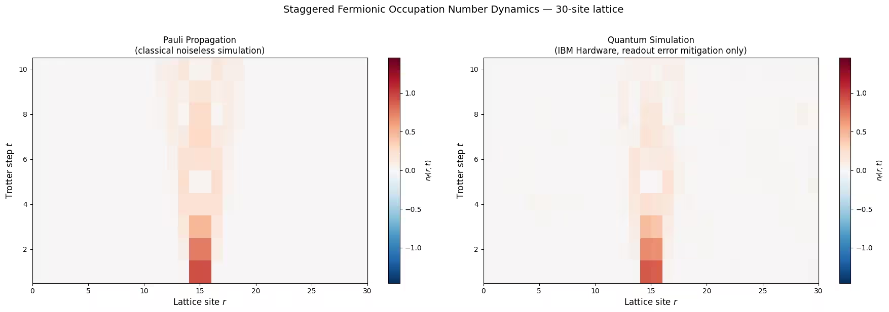
Pauli Propagation Method (PPM) ให้การจำลองแบบคลาสสิกที่ไม่มีสัญญาณรบกวนของ Circuit ควอนตัมโดยการ back-propagate observable ที่วัดได้ผ่าน Circuit ในภาพ Heisenberg ภายใต้ Clifford layer (CNOT, H, S, X gate) ตัว Pauli operator จะแมปไปยัง Pauli operator อื่นโดยไม่เพิ่มจำนวนพจน์ Non-Clifford layer (gate ใน Circuit) อาจทำให้เกิดการแตกกิ่ง — ในกรณีที่แย่ที่สุดคือทำให้จำนวนพจน์เพิ่มเป็นสองเท่า — แต่หลายกิ่งมีสัมประสิทธิ์เล็กและสามารถตัดทิ้งได้
workflow ด้วย pauli-prop คือ:
-
แยก Circuit ออกเป็นส่วน Clifford และ non-Clifford โดยใช้
evolve_through_cliffords -
Propagate แต่ละ observable ผ่านส่วน non-Clifford โดยใช้
propagate_through_circuitโดยเก็บพจน์ Pauli ไว้สูงสุดmax_termsพจน์ และทิ้งพจน์ที่มีสัมประสิทธิ์ต่ำกว่า threshold ในการตัดatol -
วิวัฒนาการ ผลลัพธ์ผ่านส่วน Clifford โดยใช้การรองรับ Clifford ที่มีอยู่ในตัวของ Qiskit
-
แยกค่า ค่าคาดหวังโดยการรวมสัมประสิทธิ์ของพจน์ Pauli แบบ diagonal (ที่มีเฉพาะ และ )
Threshold การตัด
พารามิเตอร์ atol ใน propagate_through_circuit ควบคุมความเข้มงวดในการตัดกิ่ง Pauli ที่มีค่าน้อย threshold ที่แน่นมาก (ตัวอย่างเช่น 1e-12) จะเก็บกิ่งไว้เกือบทั้งหมดและให้ผลลัพธ์ที่แม่นยำ แต่เวลาในการจำลองจะเพิ่มขึ้นอย่างรวดเร็วตามความลึกของ Circuit การจำลอง 120-qubit ในเปเปอร์ใช้เวลาประมาณ 8.5 ชั่วโมงด้วยการตั้งค่าเริ่มต้น การเพิ่ม threshold (ตัวอย่างเช่นเป็น 1e-6 หรือ 1e-3) จะทิ้งพจน์ที่มีสัมประสิทธิ์ต่ำกว่าค่านั้น ซึ่งลดจำนวนพจน์ที่ต้องติดตามลงอย่างมากและเร่งการคำนวณให้เร็วขึ้น ข้อแลกเปลี่ยนคือ error จากการประมาณค่าที่เล็กน้อยและควบคุมได้ ซึ่งคุณสามารถตรวจสอบได้โดยการเปรียบเทียบผลลัพธ์ที่ threshold ต่างกัน
import time
from pauli_prop import evolve_through_cliffords, propagate_through_circuit

# ── PPM Configuration ──
# Truncation threshold: controls the speed/accuracy trade-off.
PPM_THRESHOLD = 1e-3

# Maximum Pauli terms to track per observable (hard cap on memory/time)
PPM_MAX_TERMS = 66_000

print(f"PPM settings: atol={PPM_THRESHOLD}, max_terms={PPM_MAX_TERMS}")

# We propagate each single-qubit Z observable through each circuit.
# For PPM, we work with the un-transpiled circuits (ideal noiseless simulation).

observables_pp = [
    SparsePauliOp("I" * i + "Z" + "I" * (num_qubits_hw - i - 1))
    for i in range(num_qubits_hw)
]

def ppm_expectation_values(
    circuit, observables, max_terms=PPM_MAX_TERMS, atol=PPM_THRESHOLD
):
    """Compute expectation values of single-qubit Z observables
    via Pauli propagation.

    Args:
        circuit: The quantum circuit to simulate.
        observables: List of single-qubit Z observables.
        max_terms: Maximum number of Pauli terms to retain (hard cap).
        atol: Absolute tolerance — Pauli terms with coefficients below this
              value are discarded during propagation. Larger values give
              faster simulation at the cost of approximation accuracy.
    """
    circuit = circuit.decompose(["swap"])  # decompose SWAPs into 3 CX gates
    cliff, non_cliff = evolve_through_cliffords(circuit)

    evs = []
    for obs in observables:
        evolved_obs = propagate_through_circuit(
            obs, non_cliff, max_terms=max_terms, atol=atol, frame="h"
        )[0]
        evolved_obs.paulis = evolved_obs.paulis.evolve(cliff, frame="h")
        diagonal_mask = ~evolved_obs.paulis.x.any(axis=1)
        ev = float(evolved_obs.coeffs[diagonal_mask].sum().real)
        evs.append(ev)
    return np.array(evs)

# Run PPM for each Trotter step and record wall-clock time
pp_expvals_mid = []
pp_expvals = []
pp_times = []

for idx, d in enumerate(trotter_steps_hw):
    t_start = time.perf_counter()

    # Meson circuit
    evs_mid = ppm_expectation_values(circuits_mid_hw[idx], observables_pp)

    # Vacuum circuit
    evs_vac = ppm_expectation_values(circuits_hw[idx], observables_pp)

    elapsed = time.perf_counter() - t_start
    pp_times.append(elapsed)

    pp_expvals_mid.append(evs_mid[::-1])
    pp_expvals.append(evs_vac[::-1])

    print(f"Trotter step {d:2d}: {elapsed:.1f} s")

print(f"\nTotal PPM simulation time: {sum(pp_times):.1f} s")
print(f"Truncation threshold used: {PPM_THRESHOLD}")
PPM settings: atol=0.001, max_terms=66000
Trotter step  1: 5.0 s
Trotter step  2: 7.5 s
Trotter step  3: 11.2 s
Trotter step  4: 14.7 s
Trotter step  5: 18.3 s
Trotter step  6: 22.1 s
Trotter step  7: 25.6 s
Trotter step  8: 29.4 s
Trotter step  9: 33.2 s
Trotter step 10: 36.6 s

Total PPM simulation time: 203.6 s
Truncation threshold used: 0.001
# --- PPM simulation time vs. Trotter steps ---
fig, ax = plt.subplots(figsize=(8, 5))
ax.plot(
    list(trotter_steps_hw),
    pp_times,
    "o-",
    color="tab:blue",
    linewidth=2,
    markersize=6,
)
ax.set_xlabel("Trotter step", fontsize=13)
ax.set_ylabel("Wall-clock time (s)", fontsize=13)
ax.set_title(
    "Pauli Propagation simulation time vs. Trotter steps\n(30-site lattice, 60 qubits)",
    fontsize=13,
)
ax.grid(True, alpha=0.3)
plt.tight_layout()
plt.show()

# --- PPM heatmap and comparison with hardware ---
N_mid_pp = get_number(pp_expvals_mid, num_lattice_point_hw)
N_pp = get_number(pp_expvals, num_lattice_point_hw)
N_diff_pp = calculate_difference(N_mid_pp, N_pp, num_lattice_point_hw)

N_diff_pp_arr = np.array(N_diff_pp)

fig, axes = plt.subplots(1, 2, figsize=(18, 6))
vmax = np.abs(N_hw).max()
vmin = -vmax
norm = TwoSlopeNorm(vmin=vmin, vcenter=0, vmax=vmax)

# PPM result
im0 = axes[0].imshow(
    N_diff_pp_arr,
    aspect="auto",
    origin="lower",
    cmap="RdBu_r",
    norm=norm,
    extent=[0, num_lattice_point_hw, 0.5, len(trotter_steps_hw) + 0.5],
)
axes[0].set_xlabel("Lattice site $r$", fontsize=12)
axes[0].set_ylabel("Trotter step $t$", fontsize=12)
axes[0].set_title(
    "Pauli Propagation\n(classical noiseless simulation)", fontsize=12
)
plt.colorbar(im0, ax=axes[0], label="$n_f(r,t)$")

# Hardware result
im1 = axes[1].imshow(
    N_diff_hw_arr,
    aspect="auto",
    origin="lower",
    cmap="RdBu_r",
    norm=norm,
    extent=[0, num_lattice_point_hw, 0.5, len(trotter_steps_hw) + 0.5],
)
axes[1].set_xlabel("Lattice site $r$", fontsize=12)
axes[1].set_ylabel("Trotter step $t$", fontsize=12)
axes[1].set_title(
    "Quantum Simulation\n(IBM Hardware, readout error mitigation only)",
    fontsize=12,
)
plt.colorbar(im1, ax=axes[1], label="$n_f(r,t)$")

plt.suptitle(
    "Staggered Fermionic Occupation Number Dynamics — 30-site lattice",
    fontsize=14,
    y=1.02,
)
plt.tight_layout()
plt.show()
ขั้นตอนถัดไป
หากคุณสนใจงานนี้ ลองสำรวจเนื้อหาต่อไปนี้:
-
เอกสาร Qiskit Estimator primitive — สำหรับรายละเอียดเกี่ยวกับการตั้งค่าตัวเลือกการลด error
-
เทคนิคการลดและระงับ error — เพื่อเรียนรู้เกี่ยวกับ TREX, ZNE และวิธีการลด error อื่น ๆ
-
Qiskit Pauli Propagation (pauli-prop) — การจำลองแบบคลาสสิกที่เร่งความเร็วด้วย Rust ผ่านการ back-propagation ของ Pauli
เอกสารอ้างอิง
[1] เปเปอร์ต้นฉบับ: Ilčić, Majumdar, Mathew et al. "Observation of Robust and Coherent Non-Abelian Hadron Dynamics on Noisy Quantum Processors" arXiv:2602.18080 (2026)