จำลองการกระเจิงนิวตรอนด้วยเวิร์กโฟลว์ Serverless แบบ AQC + Trotter dynamics

ประมาณการใช้งาน: 18 นาทีบนโปรเซสเซอร์ Heron r3 (หมายเหตุ: นี่เป็นเพียงการประมาณการเท่านั้น เวลารันจริงของคุณอาจแตกต่างออกไป)

ผลลัพธ์การเรียนรู้

สเปกตรัมการกระเจิงนิวตรอนแบบไม่ยืดหยุ่น (inelastic) แมปไปยัง dynamical structure factor $S(q, \omega)$ ของแม่เหล็กควอนตัม 1 มิติได้อย่างไร
วิธีการเตรียมสถานะพื้น (ground state) ของ KCuF $_3$ (isotropic Heisenberg) ด้วย density matrix renormalization group (DMRG) และการเพิ่ม fidelity สูงสุดของ matrix product state (MPS)
วิธีการรัน Trotter time-evolution, การบีบอัด Circuit แบบ approximate quantum compilation (AQC) และการรันแบบลดผลกระทบ (mitigated execution) ในการเรียกฟังก์ชันเดียว
วิธีการประมวลผลอนุกรมเวลา $\langle \sigma_z \rangle(t)$ ต่อไซต์ให้เป็น $S(q, \omega)$ และระบุ two-spinon continuum

ข้อกำหนดเบื้องต้น

ความคุ้นเคยกับ Qiskit patterns, SparsePauliOp และ Trotter time-evolution
ความรู้พื้นฐานเกี่ยวกับวิธี tensor-network (DMRG และ MPS) จะเป็นประโยชน์แต่ไม่จำเป็น เช่นเดียวกับความคุ้นเคยกับไลบรารี qiskit-addon-aqc-tensor ที่ฟังก์ชันนี้ใช้ในการบีบอัด Circuit แบบ Trotter

ความเป็นมา

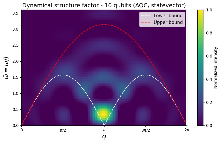
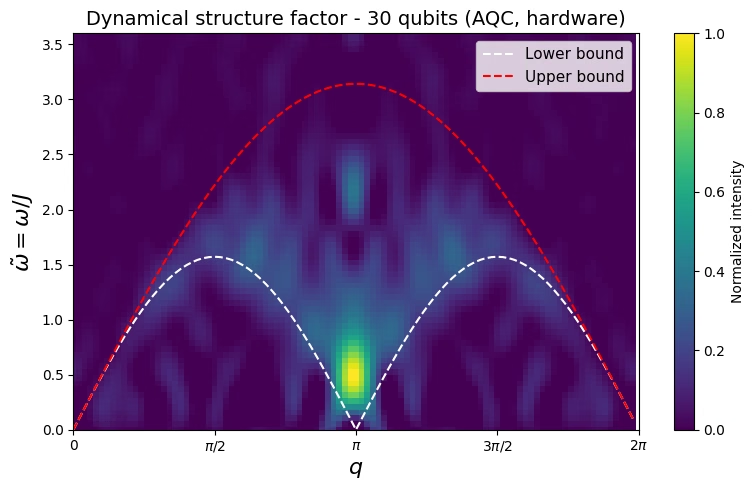
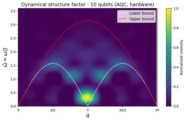
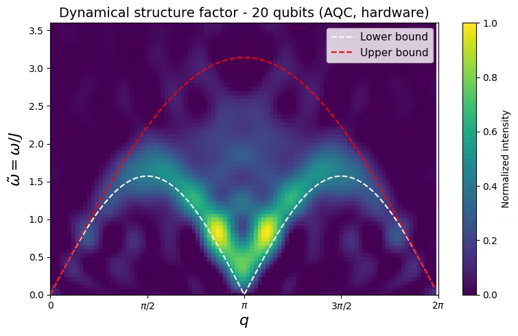
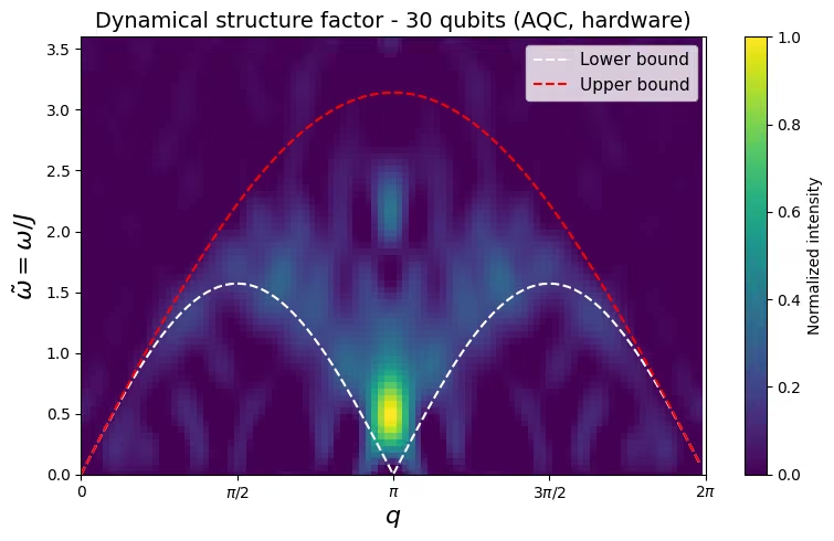
การกระเจิงนิวตรอนแบบไม่ยืดหยุ่นวัด dynamical structure factor $S(q, \omega)$ ซึ่งเป็นการแปลงฟูริเยร์ทั้งในเชิงพื้นที่และเวลาของฟังก์ชันสหสัมพันธ์สปิน-สปิน ดังนั้นการสร้าง $S(q, \omega)$ ขึ้นใหม่จากแบบจำลองสปินระดับจุลภาคจึงเป็นการทดสอบการจำลองควอนตัมที่ตรงไปตรงมาและสามารถพิสูจน์ว่าผิดได้ บทเรียนนี้ศึกษา KCuF $_3$ ซึ่งเป็นโซ่ Heisenberg แบบปฏิสัมพันธ์ต้านแม่เหล็ก (antiferromagnetic) สปิน- $\frac{1}{2}$ ที่การกระตุ้นของมันไม่ใช่การพลิกสปินเดี่ยว แต่เป็นคู่ของ spinon แบบเศษส่วน (fractionalized) แทนที่จะเป็นการกระจาย magnon ที่คมชัด $S(q, \omega)$ กลับแสดง two-spinon continuum ที่กว้าง โดยมีขอบเขตล่างที่ $\tfrac{\pi}{2}|\sin q|$ และขอบเขตบนที่ $\pi|\sin(q/2)|$ นั่นคือเส้นโค้งประที่แสดงในพล็อตต่อไปนี้ ฟิสิกส์แบบเต็มรูปแบบและการเปรียบเทียบกับข้อมูลนิวตรอนที่วัดได้ ครอบคลุมอยู่ในบทเรียนต้นฉบับ และใน Lee et al., arXiv:2603.15608

เวิร์กโฟลว์ควอนตัมสะท้อนการทดลองการกระเจิง:

เตรียมสถานะพื้นของโซ่ $|\psi_0\rangle$
กระตุ้นด้วยการรบกวนเฉพาะจุดที่ไซต์กลาง เป็นการหมุน $Z$ ขนาด $\pi/2$ เพื่อจำลองการถ่ายเทโมเมนตัมและพลังงานจากนิวตรอน
วิวัฒนาการตามเวลาภายใต้ Heisenberg Hamiltonian, $e^{-iHt}$ ด้วยสูตร Trotter product
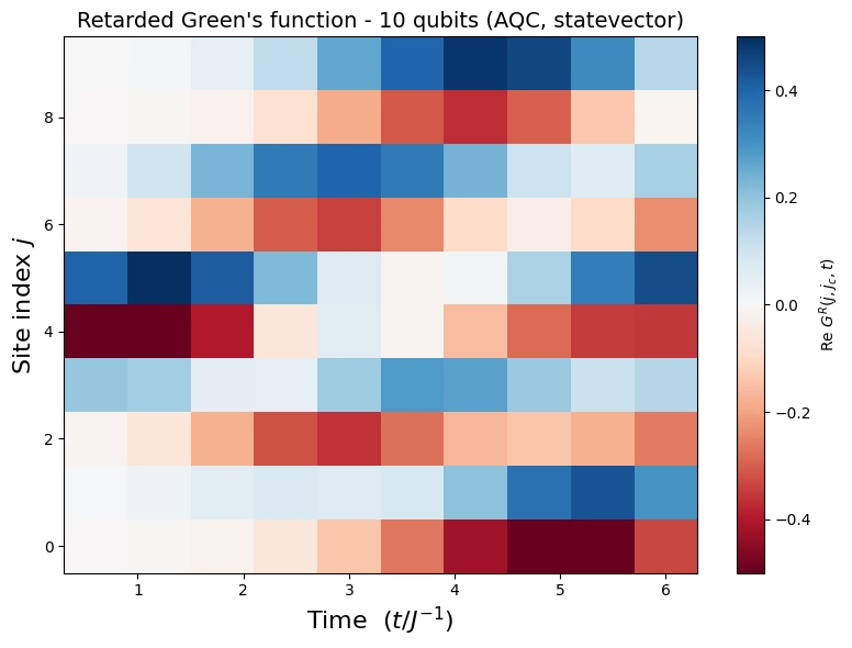
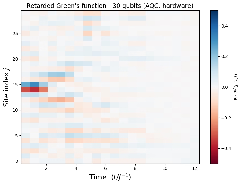
วัดค่าแมกนีไทเซชันต่อไซต์ $\langle \sigma_z^j \rangle(t)$ ในฐานะฟังก์ชันของไซต์ $j$ และเวลา $t$ นี่คือฟังก์ชันกรีนแบบหน่วงเวลา (retarded Green's function) $G^R(j, j_c, t)$ พอดี จึงไม่จำเป็นต้องแปลงก่อนการแปลงฟูริเยร์ในขั้นตอนที่ 5
แปลงฟูริเยร์ $G^R$ ให้เป็น $S(q, \omega)$

ปัญหาอาจเกิดขึ้นในขั้นตอนที่ 3 เมื่อ Circuit แบบ Trotter ที่แม่นยำสำหรับวิวัฒนาการที่ยาวนานลึกเกินไปสำหรับฮาร์ดแวร์ AQC ด้วย tensor network แก้ปัญหานี้โดยการบีบอัดบล็อกของขั้นตอน Trotter ให้เป็น ansatz แบบพารามิเตอร์ที่ตื้นและคงที่ ซึ่ง fidelity ของสถานะเทียบกับวิวัฒนาการที่แม่นยำจะถูกเพิ่มสูงสุดแบบคลาสสิกด้วย MPS simulator (arXiv:2301.08609) AQC Dynamics Template รวมแกนควอนตัมทั้งหมดนี้ (การสังเคราะห์ Trotter, การบีบอัด AQC และการรันแบบลดผลกระทบ) ไว้เบื้องหลังการเรียกครั้งเดียว:

PRE (โน้ตบุ๊กนี้)	FUNCTION (`aqc-dynamics-function`)	POST (โน้ตบุ๊กนี้)
สถานะพื้นจาก DMRG บวกกับการเพิ่ม fidelity ของ MPS สูงสุด โดยฝังการกระตุ้นนิวตรอนไว้ใน Circuit เดียวกัน	การสังเคราะห์ Trotter → การบีบอัด AQC → รันบน `statevector`, `fake`, หรือ `runtime` โดยคืนค่า $\langle \sigma_z^j \rangle(t)$ ต่อไซต์	$S(q, \omega)$ ซึ่งคือ dynamical structure factor

งานเฉพาะการทดลองยังคงอยู่ในโน้ตบุ๊กนี้ ได้แก่ การเตรียมสถานะพื้น (PRE) และการประมวลผลต่อของ $S(q, \omega)$ (POST) ส่วนสองขั้นตอนที่หนักด้านควอนตัม คือการบีบอัดและการรัน จะรันอยู่ภายในฟังก์ชัน

บทเรียนนี้เป็นบทเรียนคู่กับ Simulate neutron scattering in quantum materials with quantum circuits ซึ่งสร้างการทดลองเดียวกันแบบอินไลน์ ได้แก่ แบบจำลอง KCuF $_3$ เดียวกัน การเตรียมสถานะพื้น การกระตุ้นนิวตรอน และการประมวลผลต่อ โดยเขียนการสังเคราะห์ Trotter การบีบอัด AQC และการรันแบบลดผลกระทบไว้ทีละขั้นตอน อ่านบทเรียนนั้นเพื่อเรียนรู้ว่าการบีบอัด AQC ทำงานอย่างไร อ่านบทเรียนนี้เพื่อรันการทดลองเดียวกันผ่าน function template ที่ deploy แล้ว แกนควอนตัมกลายเป็นการเรียกฟังก์ชันเดียว และการบีบอัด AQC ที่ใช้เวลาหลายชั่วโมงจะรันภายใน Serverless worker แทนที่จะรันบนเครื่องของคุณ จึงไม่จำเป็นต้องมีระบบ HPC หรือ kernel ที่เปิดค้างไว้ระหว่างที่มันรัน การเรียกแบบเดียวกันนี้ยังขับเคลื่อนการทดลอง dynamics 1 มิติอื่น ๆ ด้วย

ข้อกำหนด

ก่อนเริ่มบทเรียนนี้ ตรวจสอบให้แน่ใจว่าคุณมีสิ่งต่อไปนี้:

ฟังก์ชันที่ deploy ไปยังบัญชี Qiskit Serverless ของคุณ รันฟังก์ชัน template คู่กันก่อน: Deploy and run the AQC + Trotter dynamics function template คู่มือนั้นจะแนะนำวิธีการรับไฟล์ source และอัปโหลดฟังก์ชันไปยังบัญชีของคุณ tutorial นี้เพียงแค่เรียกใช้ฟังก์ชันที่ deploy แล้วเท่านั้น
ข้อมูลรับรอง IBM Quantum® ที่บันทึกไว้สำหรับ QiskitServerless (ดูฟังก์ชัน template) ตัวอย่างทั้งสองใน tutorial นี้เรียกใช้ฟังก์ชันที่ deploy แล้ว ดังนั้นทั้งสองต้องใช้ข้อมูลรับรองนี้
Qiskit SDK v2.0 หรือใหม่กว่า (pip install qiskit)
Qiskit IBM Catalog client (pip install qiskit-ibm-catalog)
NumPy, SciPy และ Matplotlib (pip install numpy scipy matplotlib) จำเป็นต้องใช้ SciPy 1.14 หรือใหม่กว่าสำหรับ optimizer COBYQA ที่ใช้ในการเตรียม ground state
stack ของ AQC tensor-network เนื่องจากการเตรียม ground state ใน Step 1 รันในเครื่องภายใน notebook นี้: pip install 'qiskit-addon-aqc-tensor[quimb-jax]==0.3.1'

การเรียกครั้งแรกไปยังฟังก์ชันที่เพิ่ง deploy จะต้องรอในขณะที่ Serverless worker ติดตั้ง dependency ต่างๆ ดังนั้นให้คาดว่าจะมี latency เพิ่มขึ้นในรันนั้น

การตั้งค่า

นำเข้าไลบรารีต่างๆ และกำหนด helper เฉพาะการทดลองที่จะใช้ในภายหลัง: build_gs_ansatz (Hamiltonian variational ansatz หรือ HVA สำหรับการเตรียม ground state), prepare_ground_state (DMRG บวกกับการ maximize MPS-fidelity) และ get_spectrum, plot_green, และ plot_spectrum (การประมวลผลภายหลังของ $S(q, \omega)$ ) สิ่งเหล่านี้ดัดแปลงมาจาก original neutron-scattering tutorial

# Added by doQumentation — required packages for this notebook
!pip install -q matplotlib numpy qiskit qiskit-addon-aqc-tensor qiskit-ibm-catalog quimb scipy

from functools import partial

import matplotlib.pyplot as plt
import numpy as np
import scipy.optimize

import quimb.tensor as qtn
from qiskit import QuantumCircuit
from qiskit.quantum_info import SparsePauliOp
from qiskit_addon_aqc_tensor.simulation import tensornetwork_from_circuit
from qiskit_addon_aqc_tensor.simulation.quimb import QuimbSimulator
from qiskit_ibm_catalog import QiskitServerless

#  Dynamical structure factor via discrete Fourier transform

def get_spectrum(n, Gjjc, dt, time_steps, q_steps, w_steps):
    """Compute the dynamical structure factor from the retarded Green's function.

    Uses the center-site approximation and a discrete Fourier transform.
    """
    green = Gjjc / 4  # sigma -> S=1/2
    omega_max = np.pi / dt
    qpoints = np.arange(0, 2 * np.pi, 2 * np.pi / q_steps)
    omegas = np.arange(0, omega_max, omega_max / w_steps)
    green_map = np.zeros((omegas.shape[0], qpoints.shape[0]))
    center = n // 2 - 1
    for iw, w in enumerate(omegas):
        exponent = np.exp(1j * w * dt * np.arange(1, time_steps + 1))
        S_w = np.dot(green.T, exponent) * dt
        for iq, q in enumerate(qpoints):
            q_matrix = np.exp(-1j * q * np.arange(-center, center + 2, 1))
            green_map[iw, iq] = np.imag(np.dot(S_w, q_matrix))
    return green_map

#  Plotting helpers

def plot_spectrum(
    dsf,
    dt,
    q_steps,
    w_steps,
    lower_bound=False,
    upper_bound=False,
    title=None,
):
    """Heat-map of the dynamical structure factor."""
    omega_max = np.pi / dt
    qpoints = np.arange(0, 2 * np.pi, 2 * np.pi / q_steps)
    omegas = np.arange(0, omega_max, omega_max / w_steps)
    x, y = np.meshgrid(qpoints, omegas)
    fig, ax = plt.subplots(figsize=(8, 5))
    c = ax.pcolormesh(x, y, dsf / np.max(dsf), cmap="viridis", shading="auto")
    fig.colorbar(c, ax=ax, label="Normalized intensity")
    if lower_bound:
        ax.plot(
            qpoints,
            np.pi * np.abs(np.sin(qpoints)) / 2,
            "--",
            color="white",
            lw=1.5,
            label="Lower bound",
        )
    if upper_bound:
        ax.plot(
            qpoints,
            np.pi * np.abs(np.sin(qpoints / 2)),
            "--",
            color="red",
            lw=1.5,
            label="Upper bound",
        )
    ax.set_ylim(0, 3.6)
    ax.set_xlim(0, 2 * np.pi - 2 * np.pi / q_steps)
    ax.set_xlabel(r"$q$", fontsize=16)
    ax.set_ylabel(r"$\tilde{\omega} = \omega / J$", fontsize=16)
    ax.set_xticks([0, np.pi / 2, np.pi, 3 * np.pi / 2, 2 * np.pi])
    ax.set_xticklabels(["0", r"$\pi/2$", r"$\pi$", r"$3\pi/2$", r"$2\pi$"])
    if lower_bound or upper_bound:
        ax.legend(loc="upper right", fontsize=11)
    if title:
        ax.set_title(title, fontsize=14)
    plt.tight_layout()
    plt.show()

def plot_green(n, Gjjc, time_steps, dt, title=None):
    """Heat-map of the retarded Green's function in real space and time."""
    fig, ax = plt.subplots(figsize=(8, 6))
    t_axis = np.arange(1, time_steps + 1) * dt
    site_axis = np.arange(n)
    x, y = np.meshgrid(t_axis, site_axis)
    c = ax.pcolormesh(
        x,
        y,
        np.real(Gjjc).T,
        cmap="RdBu",
        vmax=0.5,
        vmin=-0.5,
        shading="auto",
    )
    fig.colorbar(c, ax=ax, label=r"Re $G^R(j, j_c, t)$")
    ax.set_xlabel(r"Time  ($t / J^{-1}$)", fontsize=16)
    ax.set_ylabel("Site index $j$", fontsize=16)
    if title:
        ax.set_title(title, fontsize=14)
    plt.tight_layout()
    plt.show()

#  Variational ground-state ansatz (HVA)

def _apply_xxz_pair_gate(qc, q0, q1, theta):
    """Apply the parameterized XXZ-type two-qubit gate used in the HVA."""
    qc.cx(q0, q1)
    qc.rz(theta, q1)
    qc.h(q0)
    qc.rz(theta + np.pi / 2, q0)
    qc.cx(q0, q1)
    qc.rz(-theta, q1)
    qc.h(q1)
    qc.cx(q1, q0)
    qc.rz(np.pi / 2, q1)
    qc.rz(-np.pi / 2, q0)
    qc.h(q1)
    qc.h(q0)

def build_gs_ansatz(n, params, layers):
    """Build the Hamiltonian variational ansatz (HVA) circuit for
    ground-state preparation of the 1D Heisenberg model.

    Starts from a product of singlet pairs and applies alternating
    odd/even layers of parameterized XXZ gates. For layer r,
    params[2 * r] is the odd-layer (inter-pair) angle and
    params[2 * r + 1] is the even-layer (intra-pair) angle.
    """
    qc = QuantumCircuit(n)
    # Initial singlet product state
    for i in range(n // 2):
        qc.x(2 * i)
        qc.x(2 * i + 1)
        qc.h(2 * i + 1)
        qc.cx(2 * i + 1, 2 * i)
    # Variational layers
    for r in range(layers):
        for i in range(1, (n + 1) // 2):  # odd layer
            _apply_xxz_pair_gate(qc, 2 * i - 1, 2 * i, params[2 * r])
        for i in range(n // 2):  # even layer
            _apply_xxz_pair_gate(qc, 2 * i, 2 * i + 1, params[2 * r + 1])
    return qc

def prepare_ground_state(n, gs_layers=5, max_bond=128, cutoff=1e-8):
    """Prepare the KCuF3 (isotropic Heisenberg) ground state as a QuantumCircuit.

    Runs DMRG (quimb MPO + DMRG2) to get the chain's ground state, then optimizes
    the HVA angles to maximize the MPS overlap |<psi_ansatz|psi_DMRG>|^2. No exact
    diagonalization, so it scales to larger n.
    """
    J = Jz = 1.0
    builder = qtn.SpinHam1D(S=1 / 2)
    builder += J * 0.5, "+", "-"
    builder += J * 0.5, "-", "+"
    builder += Jz, "Z", "Z"
    H_mpo = builder.build_mpo(L=n)
    dmrg = qtn.DMRG2(H_mpo)
    dmrg.solve(tol=1e-8, verbosity=0)

    gs_sim = QuimbSimulator(
        quimb_circuit_factory=partial(
            qtn.CircuitMPS, gate_opts=dict(cutoff=cutoff, max_bond=max_bond)
        ),
        autodiff_backend="jax",
    )

    def gs_infidelity(params):
        psi = tensornetwork_from_circuit(
            build_gs_ansatz(n, params, gs_layers), gs_sim
        ).psi
        return 1 - abs(psi.H @ dmrg.state) ** 2

    # Seed and optimizer match the original tutorial. Each layer starts at
    # [0, pi/2]: an odd-layer angle of 0 makes the inter-pair gate the identity,
    # and an even-layer angle of pi/2 makes the intra-pair gate a SWAP (since
    # 0.5 * (XX + YY + ZZ) = SWAP - I/2). That puts the seed at the singlet-pair
    # product limit, which is already a decent approximation to the Heisenberg
    # ground state, so the optimizer only has to refine it. The small jitter
    # (fixed RNG seed, so runs are reproducible) breaks the exact symmetry
    # between layers; COBYQA then runs for up to 100 iterations.
    rng = np.random.default_rng(12345)
    x0 = np.tile([0.0, np.pi / 2], gs_layers) + rng.normal(
        scale=0.1, size=2 * gs_layers
    )
    result_gs = scipy.optimize.minimize(
        gs_infidelity, x0, method="COBYQA", options={"maxiter": 100}
    )
    print(f"DMRG ground-state energy: {dmrg.energy:.6f}")
    print(f"GS fidelity: {1 - result_gs.fun:.4f}")
    return build_gs_ansatz(n, result_gs.x, gs_layers)

print("Setup complete - helpers defined.")

Setup complete - helpers defined.

โหลดฟังก์ชัน template

เชื่อมต่อกับ Qiskit Serverless และโหลด aqc-dynamics-function ที่ deploy แล้ว ตัวอย่างทั้งสองใน tutorial นี้เรียกใช้ handle fn เดียวกัน ดังนั้นฟังก์ชันจึงถูกโหลดเพียงครั้งเดียวที่นี่

# Credentials are read from the account saved once via QiskitServerless.save_account(...)
serverless = QiskitServerless()
fn = serverless.load("aqc-dynamics-function")

ตัวอย่าง simulator ขนาดเล็ก

ก่อนอื่นเราจะรัน workflow เต็มรูปแบบบน chain ขนาดเล็ก 10 site โดยใช้ backend statevector ที่แม่นยำ ซึ่งจะช่วยตรวจสอบความถูกต้องของ pipeline PRE → FUNCTION → POST ก่อนที่จะใช้เวลา QPU ใดๆ

Step 1: แม็ป input แบบคลาสสิกเป็นปัญหาเชิงควอนตัม

สร้าง Hamiltonian ของ KCuF $_3$ เป็น SparsePauliOp (isotropic Heisenberg: $XX + YY + ZZ$ ที่ coupling $\tfrac14$ บนแต่ละ nearest-neighbor bond; string เหล่านี้เป็น Pauli operator ดังนั้น $\tfrac14$ จึงให้ spin- $\frac{1}{2}$ coupling) เตรียม ground state ด้วย DMRG บวกกับการ maximize MPS-fidelity จากนั้นฝัง neutron kick เข้าไป: การหมุน $Z$ ขนาด $\pi/2$ ที่ center site วงจรที่เตรียมไว้คือสิ่งที่เราส่งให้ฟังก์ชันเป็น initial_state เราปล่อยให้ observables เป็นค่า default (per-site $Z$ ) ซึ่งเป็นการอ่านค่า $\langle \sigma_z^j \rangle(t)$ ที่ workflow ของ neutron ต้องการพอดี

n = 10
dt = 0.6  # physical time per Trotter step (also the omega-axis unit in POST)
time_steps = 10
center = n // 2 - 1

# MPS-simulator settings, shared by the ground-state prep here and the AQC
# compression inside the function (matches the original tutorial).
mps_max_bond = 32
mps_cutoff = 1e-8

# 1D isotropic Heisenberg (KCuF3) Hamiltonian on n qubits
H = SparsePauliOp.from_sparse_list(
    [(p, [i, i + 1], 0.25) for i in range(n - 1) for p in ("XX", "YY", "ZZ")],
    num_qubits=n,
)

# Ground state (DMRG + fidelity max) + neutron kick baked into the same circuit
gs_circuit = prepare_ground_state(
    n, gs_layers=3, max_bond=mps_max_bond, cutoff=mps_cutoff
)
gs_circuit.rz(
    np.pi / 2, center
)  # exp(-i (pi/2)/2 Z_center): the neutron perturbation
print(
    f"Prepared {n}-qubit ground state with the neutron kick at site {center}."
)

DMRG ground-state energy: -4.258035
GS fidelity: 0.9841
Prepared 10-qubit ground state with the neutron kick at site 4.

Step 2 และ 3: บีบอัดและ execute ด้วยฟังก์ชัน template

ใน workflow ที่เขียนด้วยมือ ขั้นตอนเหล่านี้จะเป็นสองขั้นตอนแยกกัน: optimize วงจรสำหรับฮาร์ดแวร์ (Step 2) และ execute วงจรเหล่านั้น (Step 3) ฟังก์ชัน template รวมทั้งสองขั้นตอนเข้าเป็นการเรียกเดียว มันทำ Trotter synthesis, AQC compression และ hardware transpilation จากนั้นรันวงจร (ที่นี่บน simulator ที่แม่นยำ ภายหลังจะใช้ error mitigation ในตัวบนฮาร์ดแวร์) พารามิเตอร์การปรับแต่งสองตัวคือ aqc_segments (แผนการบีบอัด) และ aqc_options (การตั้งค่า MPS และ optimizer) แต่ละ segment {"n_steps": k, "ansatz_steps": m} จะบีบอัด Trotter step ที่ต่อเนื่องกัน k step เข้าเป็น ansatz ที่สร้างจาก Trotter target แบบ m-step และ step ใดๆ ที่เกิน sum(n_steps) จะรันเป็น Trotter ธรรมดา step ในช่วงแรกที่มี entanglement ต่ำจะบีบอัดได้ดีเข้าสู่ ansatz แบบตื้น (ansatz_steps=1) ดังนั้นที่นี่เราจึงบีบอัดสาม step แรกเข้าเป็น ansatz ชั้นเดียว และอีกสอง step ถัดไปเข้าเป็น ansatz สองชั้นที่ลึกกว่า ส่วน Trotter step ที่เหลืออีกห้าจากทั้งหมด 10 step จะรันเป็น Trotter ธรรมดา สำหรับ aqc_options เราสะท้อนตาม tutorial ต้นฉบับ: MPS bond dimension max_bond=32, cutoff=1e-8 และ optimizer L-BFGS-B ที่จำกัดไว้ที่ 100 iteration

เรียกฟังก์ชันที่โหลดไว้ใน Setup backend="statevector" รันเส้นทางอ้างอิงที่แม่นยำ: ไม่มีการใช้เวลา QPU โดยวงจรจะรันบน statevector simulator ที่แม่นยำภายใน serverless worker (ยังคงต้องมีบัญชี Qiskit Serverless ที่บันทึกไว้เพื่อเรียกใช้) initial_state จะบรรจุ ground state ที่เตรียมไว้ (รวมถึง kick); observables ถูกละไว้เพื่อให้ฟังก์ชันวัดค่า per-site $Z$ แบบ default

job = fn.run(
    t_steps=time_steps,
    aqc_segments=[
        {
            "n_steps": 3,
            "ansatz_steps": 1,
        },  # early steps -> shallow 1-layer ansatz
        {
            "n_steps": 2,
            "ansatz_steps": 2,
        },  # later steps -> deeper 2-layer ansatz
    ],
    aqc_options={
        "max_bond": mps_max_bond,  # MPS bond dimension for AQC compression
        "cutoff": mps_cutoff,
        "optimizer_settings": {
            "method": "L-BFGS-B",
            "jac": True,
            "options": {"maxiter": 100},
        },
    },
    dt=dt,
    hamiltonian=H,
    initial_state=gs_circuit,  # prepared ground state including the neutron kick
    # observables omitted -> default per-site Z (the neutron sigma_z readout)
    backend="statevector",
)

print(job.status())  # rerun this cell until status says DONE

DONE

# The per-site <sigma_z>(t) the function returns is the retarded Green's function
# G(j, j_c, t). The workflow samples t = 1..time_steps, so drop the t = 0 row (the
# prepared+kicked state before any evolution) before post-processing.
result = job.result()
print(
    "AQC fidelities:",
    {k: round(v, 4) for k, v in result["metadata"]["aqc_fidelities"].items()},
)

ev = np.array(result["expectation_values"])
Gjjc = ev[1:]  # shape (time_steps, n)
print("Green's function shape:", Gjjc.shape)

AQC fidelities: {'1': 1.0, '2': 0.9999, '3': 0.9992, '4': 0.9998, '5': 0.9995}
Green's function shape: (10, 10)

Step 4: ประมวลผลภายหลังและคืนผลลัพธ์ในรูปแบบคลาสสิกตามต้องการ

แปลงฟูริเยร์ Green's function เป็น $S(q, \omega)$ ทำ mirror-symmetrize และตัดค่าลบทิ้ง: การประมวลผลภายหลังมาตรฐานของ neutron การทำ mirror นั้นแม่นยำเพราะ $S(q, \omega) = S(-q, \omega)$ สำหรับโมเดลนี้ และค่าลบที่เหลืออยู่เป็น artifact จากการแปลงฟูริเยร์ของ time series ที่มีขนาดจำกัดและถูกสุ่มตัวอย่างแบบไม่ต่อเนื่อง จึงถูกตัดให้เป็นศูนย์ ในรันที่แม่นยำขนาดเล็กนี้ two-spinon continuum จะถูก resolve แบบหยาบเท่านั้น แต่กลไกเหมือนกันทุกประการกับรันบนฮาร์ดแวร์ที่จะตามมา

q_res, w_res = 100, 100
spectrum = get_spectrum(n, Gjjc, dt, time_steps, q_res, w_res)
spectrum = -(spectrum + spectrum[:, ::-1]) / 2  # mirror symmetry
spectrum = np.clip(spectrum, a_min=0, a_max=None)  # clip negatives

plot_green(
    n,
    Gjjc,
    time_steps,
    dt,
    title=f"Retarded Green's function - {n} qubits (AQC, statevector)",
)
plot_spectrum(
    spectrum,
    dt,
    q_res,
    w_res,
    lower_bound=True,
    upper_bound=True,
    title=f"Dynamical structure factor - {n} qubits (AQC, statevector)",
)

Output of the previous code cell

ตัวอย่างฮาร์ดแวร์ขนาดใหญ่

workflow เดียวกันนี้ขยายขนาดขึ้นได้โดยไม่ต้องเปลี่ยนโค้ดวิทยาศาสตร์เลย: chain ขนาด 30 site, Trotter depth เป็นสองเท่า (20 step), แผนการบีบอัดที่ปรับความลึกของ ansatz ให้แตกต่างกัน (ansatz ที่ลึกกว่าสำหรับ step ที่มี entanglement มากกว่าในช่วงหลัง) และการ execute บนโปรเซสเซอร์ IBM Quantum พร้อม error mitigation ในตัวของฟังก์ชัน (dynamical decoupling, Pauli twirling และ twirled readout error extinction (TREX)) เราจะเดินผ่านสี่ step เดียวกันกับตัวอย่าง simulator โดยใช้ handle fn จาก Setup ซ้ำ

	ขนาดเล็ก	ขนาดใหญ่
Qubit	10	30
Trotter step	10	20
AQC-compressed step (1-layer + 2-layer)	3 + 2 = 5	6 + 4 = 10
ชั้น ansatz ของ ground state	3	5
MPS max bond dimension	32	128
Backend	`statevector`	QPU พร้อม DD, Pauli twirling และ TREX

Step 1: แม็ป input แบบคลาสสิกเป็นปัญหาเชิงควอนตัม

สร้าง SparsePauliOp ของ Heisenberg KCuF $_3$ เดียวกันและเตรียม ground state โดยตอนนี้ใช้ ansatz gs_layers=5 ที่ลึกกว่าสำหรับ chain ที่ยาวกว่า จากนั้นฝัง neutron kick $Z$ ขนาด $\pi/2$ ที่ center site วิธีการนี้เหมือนกับการแม็ปในขนาดเล็กทุกประการ เพียงแต่ที่ $n = 30$

คาดว่า ground-state fidelity จะต่ำกว่ารันแบบ 10 site: ประมาณ 0.82 ที่นี่ เทียบกับ 0.98 สำหรับ chain ขนาดเล็กกว่า เนื่องจากชั้น HVA ทั้งห้าไม่สามารถจับ ground state ของ 30 site ได้อย่างสมบูรณ์ นี่เป็นเรื่องที่คาดไว้แล้วไม่ใช่ความล้มเหลว และ tutorial ต้นฉบับก็ยอมรับค่าประมาณ 0.65 ที่ 50 site ด้วยเหตุผลเดียวกัน การเพิ่ม gs_layers หรือขีดจำกัด iteration ของ COBYQA จะช่วยปรับปรุงค่านี้ โดยแลกกับต้นทุนการคำนวณแบบคลาสสิกเพิ่มเติม

n = 30
dt = 0.6
time_steps = 20
center = n // 2 - 1

# Same MPS settings as the original large-scale run: a larger bond for the
# longer, more-entangled chain (shared by GS prep and AQC compression).
mps_max_bond = 128
mps_cutoff = 1e-8

# Same KCuF3 Hamiltonian and ground-state prep, on a larger chain
H = SparsePauliOp.from_sparse_list(
    [(p, [i, i + 1], 0.25) for i in range(n - 1) for p in ("XX", "YY", "ZZ")],
    num_qubits=n,
)
gs_circuit = prepare_ground_state(
    n, gs_layers=5, max_bond=mps_max_bond, cutoff=mps_cutoff
)
gs_circuit.rz(np.pi / 2, center)  # neutron kick at the center site
print(
    f"Prepared {n}-qubit ground state with the neutron kick at site {center}."
)

DMRG ground-state energy: -13.111355
GS fidelity: 0.8201
Prepared 30-qubit ground state with the neutron kick at site 14.

Step 2 และ 3: บีบอัดและ execute ด้วยฟังก์ชัน template

การเรียกเดียวแบบเดียวกับตัวอย่าง simulator ตอนนี้ให้ backend_name ชี้ไปที่โปรเซสเซอร์ IBM Quantum ดังนั้นฟังก์ชันจะ transpile และ execute ที่นั่น แผนการบีบอัดปรับความลึกของ ansatz ให้แตกต่างกัน: Trotter step หกแรก (ที่มี entanglement ต่ำ) บีบอัดเข้าเป็น ansatz ชั้นเดียวแบบตื้น สี่ step ถัดไปเข้าเป็น ansatz สองชั้นที่ลึกกว่า และ step ที่เหลืออีก 10 จากทั้งหมด 20 step รันเป็น Trotter ธรรมดา aqc_options เพิ่ม MPS bond dimension เป็น max_bond=128 สำหรับ chain ที่ยาวกว่าและมี entanglement มากกว่า (สอดคล้องกับต้นฉบับ) โดยยังคง optimizer L-BFGS-B ที่จำกัด 100 iteration เหมือนเดิม estimator_options เปิดใช้งาน error mitigation ในตัว: dynamical decoupling (XY4), gate twirling และ TREX measurement mitigation ค่า default ของฟังก์ชันตรงกับ tutorial ต้นฉบับอยู่แล้วสำหรับทั้งหมดนี้ ยกเว้น budget การเรียนรู้ของ TREX (measure_noise_learning) เราจึงยังเขียน block ทั้งหมดออกมาเพราะ estimator_options ที่ผู้เรียกใช้ให้มาจะแทนที่ default ของฟังก์ชันทั้งหมดแทนที่จะ merge เข้าไป ดังนั้นการละ key ใดไปจะทำให้ตกไปใช้ default ของ IBM Quantum Compute แทนที่จะเป็นของฟังก์ชัน

# Steps 2 + 3: the function compresses (varied ansatz) and executes on hardware.
job = fn.run(
    t_steps=time_steps,
    aqc_segments=[
        {
            "n_steps": 6,
            "ansatz_steps": 1,
        },  # early steps -> shallow 1-layer ansatz
        {
            "n_steps": 4,
            "ansatz_steps": 2,
        },  # later steps -> deeper 2-layer ansatz
    ],
    aqc_options={
        "max_bond": mps_max_bond,  # 128 for the longer chain
        "cutoff": mps_cutoff,
        "optimizer_settings": {
            "method": "L-BFGS-B",
            "jac": True,
            "options": {"maxiter": 100},
        },
    },
    dt=dt,
    hamiltonian=H,
    initial_state=gs_circuit,
    backend_name="ibm_pittsburgh",
    # Mitigation settings from the original tutorial. Only the two
    # measure_noise_learning values differ from the function's defaults; the rest
    # restates them, because a caller-supplied estimator_options dict replaces the
    # function's defaults wholesale rather than merging into them.
    estimator_options={
        "environment": {"job_tags": ["TUT-SNS"]},
        "dynamical_decoupling": {"enable": True, "sequence_type": "XY4"},
        "twirling": {
            "enable_gates": True,
            "num_randomizations": 1000,
            "shots_per_randomization": 128,
        },
        "resilience": {
            "measure_mitigation": True,
            "measure_noise_learning": {
                "num_randomizations": 32,
                "shots_per_randomization": 100,
            },
        },
    },
)
print("job ID (save this to reconnect later):", job.job_id)

job ID (save this to reconnect later): 43ed8d07-6d7d-4f33-b70a-7f31b765b310

การเชื่อมต่อใหม่กับ job ที่รันนาน

รันขนาดใหญ่นี้ไม่เร็ว และเวลาส่วนใหญ่เป็นการคำนวณแบบคลาสสิกไม่ใช่บน QPU การบีบอัด AQC รันภายในฟังก์ชันก่อนที่จะไปถึง QPU: ที่ 30 site ด้วย max_bond=128 ใช้เวลาเกือบสี่ชั่วโมงในรันของเรา เทียบกับเวลา QPU ประมาณ 18 นาทีที่ระบุใน ประมาณการการใช้งาน ที่ด้านบนของ tutorial นี้ เวลารอคิวจะเพิ่มเติมจากทั้งสองส่วนนี้ คุณไม่จำเป็นต้องเปิด notebook หรือ kernel นี้ค้างไว้ในขณะที่มันรัน

คัดลอก job ID ที่พิมพ์ออกมาจาก cell ก่อนหน้าและบันทึกไว้ สาม cell ถัดไปช่วยให้คุณกลับมาทำงานต่อได้ในภายหลัง:

เชื่อมต่อใหม่ จำเป็นเฉพาะใน kernel session ใหม่: รัน cell Setup อีกครั้งเพื่อสร้าง serverless ขึ้นใหม่ จากนั้นสร้าง handle ของ job ขึ้นใหม่จาก ID ที่คุณบันทึกไว้ ข้าม cell นี้ไปหากคุณยังอยู่ใน session เดียวกับที่คุณส่ง job เพราะ handle นั้นยังคงใช้งานได้อยู่
ตรวจสอบสถานะ: รันซ้ำจนกว่าจะรายงาน DONE
ดึงผลลัพธ์: รันเฉพาะเมื่อสถานะเป็น DONE แล้วเท่านั้น

cell การเชื่อมต่อใหม่ต่อไปนี้มี placeholder อยู่ แทนที่ด้วย job_id ของคุณเอง:

# Reconnect to a previously submitted job by its ID. Only needed in a NEW kernel
# session; if you are still in the session where you submitted, the `job` handle
# from the preceding cell is already live, so skip this cell. Replace the ID that follows with your own.
job = serverless.get_job_by_id("<your job ID>")

# Check where the job is. Re-run this until it reports DONE before fetching the
# result in the following cell: QUEUED -> INITIALIZING -> RUNNING: OPTIMIZING_FOR_HARDWARE ->
# RUNNING: WAITING_FOR_QPU -> RUNNING: EXECUTING_QPU -> RUNNING: POST_PROCESSING
# -> DONE.
print(job.status())

DONE

# Run this only once the preceding status cell reports DONE. result() blocks until
# the job finishes, so calling it earlier just waits (possibly for hours).
result = job.result()
print(
    "AQC fidelities:",
    {k: round(v, 4) for k, v in result["metadata"]["aqc_fidelities"].items()},
)

ev = np.array(result["expectation_values"])
Gjjc = ev[1:]  # drop the t = 0 row -> shape (time_steps, n)

AQC fidelities: {'1': 1.0, '2': 0.9994, '3': 0.9944, '4': 0.9853, '5': 0.9747, '6': 0.959, '7': 0.9495, '8': 0.9542, '9': 0.9533, '10': 0.9451}

Step 4: ประมวลผลภายหลังและคืนผลลัพธ์ในรูปแบบคลาสสิกตามต้องการ

การประมวลผลภายหลังเหมือนกับรัน simulator ทุกประการ: แปลงฟูริเยร์ Green's function เป็น $S(q, \omega)$ ทำ mirror-symmetrize และตัดค่าลบทิ้ง ด้วย chain และการวิวัฒนาการที่ยาวกว่า two-spinon continuum จะถูก resolve ได้ดีกว่ามาก ควรจะเติมเต็มแถบระหว่างขอบเขตเส้นประ โดยสว่างที่สุดใกล้ $q = \pi$

n = result["metadata"]["n"]
q_res, w_res = 100, 100
spectrum = get_spectrum(n, Gjjc, dt, time_steps, q_res, w_res)
spectrum = -(spectrum + spectrum[:, ::-1]) / 2  # mirror symmetry
spectrum = np.clip(spectrum, a_min=0, a_max=None)  # clip negatives

plot_green(
    n,
    Gjjc,
    time_steps,
    dt,
    title=f"Retarded Green's function - {n} qubits (AQC, hardware)",
)
plot_spectrum(
    spectrum,
    dt,
    q_res,
    w_res,
    lower_bound=True,
    upper_bound=True,
    title=f"Dynamical structure factor - {n} qubits (AQC, hardware)",
)

Output of the previous code cell

ภาคผนวก

ตัวอย่างฮาร์ดแวร์ก่อนหน้านี้รัน chain ความยาวเดียว สเปกตรัมทั้งสามที่ตามมาต่อไปนี้มาจากรันฮาร์ดแวร์ก่อนหน้าของ workflow เดียวกันนี้บน ibm_pittsburgh ที่ 10, 20 และ 30 site โดยที่ input อื่นทั้งหมดคงที่: Trotter step 20 step ที่ dt = 0.6 แผนการบีบอัดแบบ AQC: หก step ด้วย ansatz ชั้นเดียว บวกอีกสี่ step ด้วย ansatz สองชั้น และ max_bond = 128 เหล่านี้เป็นผลลัพธ์ที่บันทึกไว้ ไม่ใช่ output จาก cell ก่อนหน้า

ใช้การตั้งค่าเดียวกันในทั้งสามขนาด ดังนั้นสเปกตรัมจึงเปรียบเทียบกันได้โดยตรง การปรับแต่งตามความยาว chain แต่ละแบบ เช่น ด้วยชั้น ansatz ของ ground state ที่มากขึ้น หรือ max_bond ที่ใหญ่ขึ้น สามารถให้ผลลัพธ์ที่ดีกว่าที่แสดงไว้ที่นี่ได้

Dynamical structure factor at 10 sites, a single sharp bright peak at q = pi near the lower bound

Dynamical structure factor at 20 sites, spectral weight filling the band between the two dashed two-spinon bounds

Dynamical structure factor at 30 sites, the continuum resolved more finely with fainter contrast and some weight outside the bounds

ขั้นตอนถัดไป

คำแนะนำ

ปรับ workflow นี้ให้เข้ากับระบบของคุณเอง: ฟังก์ชันรองรับ SparsePauliOp แบบ 1D nearest-neighbor ใดๆ ดังนั้น chain Hamiltonian, initial state หรือชุด observable ที่แตกต่างกันจะรัน pipeline PRE → FUNCTION → POST แบบเดียวกัน ดู contract ของ input/output แบบเต็มได้ใน AQC Dynamics Template on GitHub
อ่านงานวิจัยที่ benchmark นี้มาจาก: Lee et al., Benchmarking quantum simulation with neutron-scattering experiments (arXiv:2603.15608)
เปรียบเทียบกับ tutorial "Simulate neutron scattering" ต้นฉบับ ซึ่งเป็น workflow แบบ inline ที่ tutorial นี้นำมาย้ายไปใช้กับฟังก์ชัน template ที่ deploy แล้ว
เจาะลึกเพิ่มเติมเกี่ยวกับ เทคนิคการลด (mitigation) และระงับ (suppression) ข้อผิดพลาด ที่ใช้ในรันฮาร์ดแวร์: dynamical decoupling, Pauli twirling และ TREX

ผลลัพธ์การเรียนรู้​

ข้อกำหนดเบื้องต้น​

ความเป็นมา​

ข้อกำหนด​

การตั้งค่า​

โหลดฟังก์ชัน template​

ตัวอย่าง simulator ขนาดเล็ก​

Step 1: แม็ป input แบบคลาสสิกเป็นปัญหาเชิงควอนตัม​

Step 2 และ 3: บีบอัดและ execute ด้วยฟังก์ชัน template​

Step 4: ประมวลผลภายหลังและคืนผลลัพธ์ในรูปแบบคลาสสิกตามต้องการ​

ตัวอย่างฮาร์ดแวร์ขนาดใหญ่​

Step 1: แม็ป input แบบคลาสสิกเป็นปัญหาเชิงควอนตัม​

Step 2 และ 3: บีบอัดและ execute ด้วยฟังก์ชัน template​

Step 4: ประมวลผลภายหลังและคืนผลลัพธ์ในรูปแบบคลาสสิกตามต้องการ​

ภาคผนวก​

ขั้นตอนถัดไป​

ผลลัพธ์การเรียนรู้

ข้อกำหนดเบื้องต้น

ความเป็นมา

ข้อกำหนด

การตั้งค่า

โหลดฟังก์ชัน template

ตัวอย่าง simulator ขนาดเล็ก

Step 1: แม็ป input แบบคลาสสิกเป็นปัญหาเชิงควอนตัม

Step 2 และ 3: บีบอัดและ execute ด้วยฟังก์ชัน template

Step 4: ประมวลผลภายหลังและคืนผลลัพธ์ในรูปแบบคลาสสิกตามต้องการ

ตัวอย่างฮาร์ดแวร์ขนาดใหญ่

Step 1: แม็ป input แบบคลาสสิกเป็นปัญหาเชิงควอนตัม

Step 2 และ 3: บีบอัดและ execute ด้วยฟังก์ชัน template

Step 4: ประมวลผลภายหลังและคืนผลลัพธ์ในรูปแบบคลาสสิกตามต้องการ

ภาคผนวก

ขั้นตอนถัดไป